Modeling and Numerical Approximation of Traffic Flow Problems
Prof. Dr. Ansgar J¨ ungel Universit¨at Mainz
Lecture Notes (preliminary version) Winter 2002
Contents
1 Introduction 1
2 Mathematical theory for scalar conservation laws 4
3 Traffic flow models 13
4 Numerical approximation of scalar conservation laws 16
5 The Gudonov method 27
References 32
1 Introduction
The goal of these lecture notes is to introduce to the modeling of car traffic flow using con- servation laws and to the numerical discretization of the resulting hyperbolic differential equations.
Consider the traffic flow of cars on a highway with only one lane (i.e., overtaking is impossible). Instead of modeling the cars individually, we use the density ρ(x, t) of cars (in vehicles per kilometer, say) in x∈ R at timet ≥0. The number of cars which are in the interval (x1, x2) at time t is Z x2
x1
ρ(x, t)dx.
Let v(x, t) denote the velocity of the cars in x at time t. The number of cars which pass throughxat timet(in unit length) isρ(x, t)v(x, t). We want to derive an equation for the evolution of the car density. The number of cars in the interval (x1, x2) changes according to the number of cars which enter or leave this interval (see Figure 1.1):
d dt
Z x2
x1
ρ(x, t)dx=ρ(x1, t)v(x1, t)−ρ(x2, t)v(x2, t).
Integration of this equation with respect to time and assuming that ρ and v are regular functions yields
Z t2
t1
Z x2
x1
∂tρ(x, t)dx dt = Z t2
t1
(ρ(x1, t)v(x1, t)−ρ(x2, t)v(x2, t)) dx dt
= −
Z t2
t1
Z x2
x1
∂x(ρ(x, t)v(x, t)) dx dt.
Since x1, x2 ∈R,t1, t2 >0 are arbitrary, we conclude
ρt+ (ρv)x = 0, x∈R, t >0. (1.1) This is a partial differential equation. It has to be supplemented by the initial condition
ρ(x,0) =ρ0(x), x∈R. (1.2)
cars ρ 2(x ,t) v(x ,t)2
(x ,t) v(x ,t) ρ 1
1
Figure 1.1: Derivation of the conservation law.
We also need an equation for the velocity v. We assume that v only depends on ρ (see Section 3 for other choices). If the highway is empty (ρ = 0), we will drive with maximal velocity v = vmax; in heavy traffic we will slow down and will stop (v = 0) in a tailback where the cars are bumper to bumper (ρ =ρmax). The simplest model is the linear relation
v(ρ) = vmax
µ
1− ρ ρmax
, 0≤ρ≤ρmax. Equation (1.1) then becomes
ρt+
· vmaxρ
µ
1− ρ ρmax
¶¸
x
= 0, x∈R, t >0. (1.3)
This equation is a so-called conservation law since it expresses the conservation of the number of cars. Indeed, integrating (1.3) formally overx∈R gives
d dt
Z
Rρ(x, t)dx=− Z
R
∂
∂x
·
vmaxρ(x, t) µ
1− ρ(x, t) ρmax
¶¸
dx= 0, and thus the number of cars inR is constant for all t≥0.
Equation (1.3) belongs to the class of hyperbolic equations. We call a system of equa- tions
∂tu+∂xf(u) = 0, x∈R, t >0, (1.4)
u(x,0) = u0(x), x∈R, (1.5)
withf :Rm →Rm hyperbolicif and only if for anyu∈Rm,f0(u) can be diagonalized and has only real eigenvalues. A function u:R×[0,∞)→Rm is called a classical solutionof (1.4)–(1.5) if u∈C1(R×(0,∞))∩C0(R×[0,∞)) and u solves (1.4)–(1.5) pointwise.
Equation (1.3) can be simplified by bringing it in a dimensionless form. Let L and τ be a typical length and time, respectively, such that L/τ =vmax. Introducing
xs = x
L, ts = t
τ, u= 1− 2ρ ρmax, we obtain
∂tρ= 1 τ∂ts
hρmax
2 (1−u)i
=−ρmax
2τ ∂tsu,
∂x
· vmaxρ
µ
1− ρ ρmax
¶¸
= 1 L∂xs
· vmax
ρmax
2 (1−u)1
2(1 +u)
¸
=−ρmax
2τ ∂xs
µu2 2
¶ , and hence we can write (1.2)–(1.3) as (with (x, t) instead of (xs, ts))
ut+ µu2
2
x
= 0, x∈R, t >0, (1.6)
u(x,0) = u0(x), x∈R, (1.7)
with u0 = 1−2ρ0/ρmax. If the highway is empty (ρ = 0), we have u = 1; in a tailback (ρ=ρmax),u=−1 holds. Equation (1.6) is also called the inviscid Burgers equation.
In order to see how the solutions of (1.6) may look like, consider the following example.
Let
u0(x) =
1 : x <0 1−x : 0≤x <1
0 : x≥1,
(1.8) i.e., there are initially no cars in x < 0 and a moderate traffic in x ≥ 1. What happens for t >0? It is easy to check that
u(x, t) =
1 : x < t
1−t−x
1−2t : t≤x <1−t 0 : x≥1−t
is a solution of (1.6)–(1.7) for x ∈ R, t < 1/2 which satisfies (1.4) pointwise except at x = 1 and x = 1 −t (see Figure 1.2). The solution becomes discontinuous at t = 1.
1 4
1 2
1 2 t = 0
1
t = t =
0
1 x
Figure 1.2: Solution of (1.6)–(1.8).
The cars which were initially in (0,1) drive from the left to the right until no cars were remaining in that interval. Asu= 0 in x <0, no other cars are coming.
This gives rise to the following questions:
• Does there exist any solution for t≥1/2?
• If yes, how does the solution for t≥1/2 look like?
• How can we solve (1.6)–(1.7) for more complicated intial data numerically?
It is clear that we need some theory before we can turn to the numerical treatment of hyperbolic conservation laws.
2 Mathematical theory for scalar conservation laws
In this section we study the problem
ut+f(u)x = 0, x∈R, t >0, (2.1)
u(x,0) = u0(x), x∈R, (2.2)
for some function f :R→R. This problem can be solved using themethod of character- istics.
Definition 2.1 Let u: [0, T)→R be a (classical) solution of (2.1)–(2.2). The solutions χ of the initial-value problem
χ0(t) = f0(u(χ(t), t)), t >0, χ(0) =x0 are called the characteristics of (2.1).
The main property of the characteristics is that u is constant along them:
d
dtu(χ(t), t) =ut(χ(t), t) +ux(χ(t), t)χ0(t) = 0, t >0, and hence u(χ(t), t) = const. for t >0.
Example 2.2 Letf(u) = u2/2. The characteristics of (2.1) are given as the solutions of χ0(t) =u(χ(t), t), t >0, χ(0) =x0.
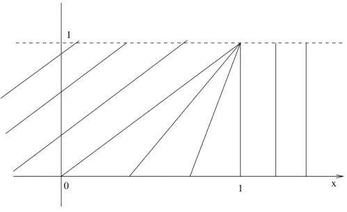
As u(χ(t), t) = const. for t > 0, χ is a straight line in the (x, t)-plane through x0 with slope 1/u0(χ(t)) = 1/u0(x0). Characteristics allow to illustrate the solutions of (1.6)–
(1.7) in a compact form. An example with u0 as in (1.8) is given in Figure 2.1. The characteristics should notbe confused with the vehicle trajectories; they rather illustrate
the “propagation” of the density values. ¤
0 1 x
1
Figure 2.1: Characteristics of (1.6)–(1.8).
Example 2.2 shows again that solutions of (2.1)–(2.2) may develop discontinuities after finite time. Therefore we need a solution concept including discontinuous functions. For
this, let u be a classical solution of (2.1)–(2.2); multiplying (2.1) by φ ∈ C01(R2) = {φ ∈ C1(R2) :φ has compact support} and integrating over R2 yields
0 = Z ∞
0
Z
R(ut+f(u)x)φ dx dt
= −
Z ∞
0
Z
R(uφt+f(u)φx)dx dt− Z
Ru(x,0)φ(x,0)dx.
In order to define the last two integrals we only need integrable functionsu! This motivates the following definition.
Definition 2.3 The function u:R×(0, T)→R is called a weak solution of (2.1)–(2.2) if for all φ∈C01(R2)
Z ∞
0
Z
R(uφt+f(u)φx)dx dt=− Z
Ru0(x)φ(x,0)dx.
Implicitely, this definition includes some regularity requirements on u (for instance, integrability of u and f(u)), but we do not specify them. It is not difficult to check that each classical solution is a weak solution, but the inverse does not need to be true.
Another weak formulation of (2.1) can be obtained as follows. Let u be a classical solution of (2.1)–(2.2). Integrating (2.1) over (a, b)×(s, t) for any a, b∈ R and s, t > 0 gives
Z b
a
u(x, t)dx− Z b
a
u(x, s)dx=− Z t
s
f(u(b, τ))dτ + Z t
s
f(u(a, τ))dτ. (2.3) Then we can say thatuis a weak solution of (2.1)–(2.2) ifu(·,0) =u0 and (2.3) is satisfied for all a, b ∈ R, s, t > 0. It is possible to prove that any weak solution in the sense of Definition 2.3 also satisfies (2.3), but we do not present the (technical) proof.
We now consider conservation laws with special discontinuous initial data.
Definition 2.4 The problem (2.1)–(2.2) with initial datum u0(x) =
( u` : x <0
ur : x≥0 (2.4)
and u`, ur∈R is called a Riemann problem.
We want to solve the Riemann problem (2.1)–(2.2), (2.4). For this, we observe that with u(x, t) also u(αx, αt) is a solution of (2.1)–(2.2), (2.4) for any α > 0. Therefore, u only depends on ξ=x/t, i.e. u=u(ξ). This implies
0 = ut+f(u)x = −x
t2u0(ξ) +f0(u(ξ))u0(ξ)1 t = 1
tu0(ξ)(f0(u(ξ))−ξ).
Now several possibilities can occur:
• u0(ξ) = 0 =⇒ u(ξ) = const.
• f0(u(ξ)) =ξ =⇒ u(ξ) = (f0)−1(ξ) (if the inverse of f0 exists; a sufficient condition is f00 >0 in R).
• u is discontinuous along ξ=x/t, i.e., u0(ξ) does not exist.
This observation motivates to consider three cases:
Case 1: u`=ur. This gives the solution u(x, t) = ur =u` for all x∈R, t >0.
Case 2: u` > ur. For f(u) = u2/2, a traffic flow interpretation is that the vehicle density in x > 0 is larger than in x < 0. As the flow direction is from the left to the right, we expect a shock line, i.e. a discontinuity curve x = ψ(t). We claim that the discountinuous function
u(x, t) =
( u` : x < st
ur : x≥st (2.5)
is a weak solution of (2.1)–(2.2), (2.4). Then the discontinuity line is given byx=ψ(t) = st and s = ψ0(t) is the shock speed which has to be determined. In order to prove our claim let φ∈C01(R2). Then, since u= const. except on x=st,
Z ∞
0
Z
Ruφtdx dt = Z ∞
0
µZ st
−∞
uφtdx+ Z ∞
st
uφtdx
¶ dt
= Z ∞
0
³
∂t
Z st
−∞
uφ dx−s·u(st−0, t)φ(st, t) +∂t
Z ∞
st
uφ dx+s·u(st+ 0, t)φ(st, t)´ dt
= −
Z
Ru(x,0)φ(x,0)dx−s·(u`−ur) Z ∞
0
φ(st, t)dt and, by integration by parts,
Z ∞
0
Z
Rf(u)φxdx dt = Z ∞
0
³
− Z st
−∞
f(u)xφ dx+f(u(st−0, t))φ(st, t)
− Z ∞
st
f(u)xφ dx−f(u(st+ 0, t))φ(st, t)´ dt
= (f(u`)−f(ur)) Z ∞
0
φ(st, t)dt.
We conclude Z ∞
0
Z
R(uφt+f(u)φx) dx dt = − Z
Ru0(x)φ(x,0)dx
−[s·(u`−ur)−(f(u`)−f(ur))]
Z ∞
0
φ(st, t)dt.
Thus, choosing
s = f(u`)−f(ur) u`−ur
, (2.6)
we have proved the claim.
The choice (2.6) is called the Rankine-Hugoniot condition. For a Riemann problem, s is always a constant, i.e., the discontinuity curve is always a straight line. This may not be true for general initial data. In this situation, the Rankine-Hugoniot condition generalizes to [4, Sec. 106]
s(t) =ψ0(t) = f(u`(t))−f(ur(t))
u`(t)−ur(t) , (2.7)
where
u`(t) = lim
x%ψ(t)u(x, t), ur(t) = lim
x&ψ(t)u(x, t). (2.8)
It can be shown that (2.5) is the unique weak solution of (2.1)–(2.2) (see Theorem 2.9).
Example 2.5 Let f(u) = u2/2 and u` = 0, ur = −1. Then the shock speed is s =
1
2(u`+ur) = −12, and the solution of (2.1)–(2.2), (2.4) is illustrated in Figure 2.2. The traffic flow interpretation is the following. Inx < st=−t/2, cars with a moderate density are coming from the left and stop at the tailback at x=−t/2. In x >−t/2, the density is maximal and the cars are bumper to bumper and are not moving. The shock line
x=−t/2 denotes the beginning of the tailback. ¤
t
x
Figure 2.2: Characteristics for (1.6)–(1.7) with u` = 0, ur =−1.
Case 3: u` < ur. For this case we assume that f00 >0 in R. One solution is given by (2.5), as the above proof does not need a sign on u`−ur:
u1(x, t) =
( u` : x < st ur : x≥st.
It can be shown that also
u2(x, t) =
u` : x < f0(u`)t
(f0)−1(x/t) : f0(u`)t ≤x≤f0(ur)t ur : x > f0(ur)t
is a weak solution (motivated by the computation before Case 1; see Figure 2.3). In fact, it is possible to show that the problem (2.1)–(2.2), (2.4) possesses infinitely many weak solutions! (See, for instance, [5, Sec. 3.5].) What is the physically relevant solution? We present two approaches.
t
x 0
t
x 0
Figure 2.3: Characteristics for (2.1)–(2.2), (2.4) with f(u) = u2/2 and u` = 0, ur = 1, corresponding to u1 (left) and u2 (right).
In the traffic flow interpretation, the conditionu` < ur means that there are more cars (per kilometer) in {x < 0} than in {x > 0}. The solution u1 would mean that all cars in {x < st} drive with the same velocity v(u`) = vmax(1 +u`)/2, whereas all drivers in {x > st} move with the velocity v(ur)> v(u`), and there is a shock at x =st. It would be more realistic if the drivers just before the shock line (x <0) tried to drive as fast as the drivers behind the shock (x > 0). After some time there are drivers with velocities v(u`) and v(ur) far away from x = 0 and some drivers with velocities between v(u`) and v(ur) near x= 0. Thus,u2 seems to be the preferable physical solution. The solution u2 is called rarefaction wave.
Is it possible to formulate a general principle which allows to select the physically correct solution? The answer is yes and this leads to the notion of entropy condition.
Definition 2.6 A weak solution u : R×(0, T) → R of (2.1)–(2.2), (2.4) satisfies the entropy condition of Oleinik if and only if along each discontinuity curve x=ψ(t),
f(u`(t))−f(v)
u`(t)−v ≥ψ0(t)≥ f(ur(t))−f(v)
ur(t)−v (2.9)
for all t ∈ (0, T) and for all v between u`(t) and ur(t), where u`(t), ur(t) are defined in (2.8).
Does u1 satisfy the entropy condition (2.9)? Since ψ0(t) = s(t) = f(ur)−f(u`)
ur−u`
and f is assumed to be strictly convex, we obtain for any u` < v < ur
f(u`)−f(v)
u`−v < f(u`)−f(ur) u`−ur
=s < f(ur)−f(v) ur−v ,
which contradicts (2.9). Thus, u1 does not satisfy the entropy condition (2.9). The function u of Case 2, defined in (2.5), however, satisfies (2.9) (if f is convex). As the function u2 is continuous, we do not need to check (2.9) for this function.
The second approach uses the notion of entropy. We call a function η ∈ C2(R) an entropy and ψ ∈ C1(R) an entropy flux if and only if η is strictly convex and if for any classical solution u of (2.1)–(2.2) it holds
η(u)t+ψ(u)x = 0, x∈R, t >0. (2.10) The idea of the second approach is to consider the conservation law as an idealization of a diffusive problem given by the equation
ut+f(u)x =εuxx, x∈R, t >0, (2.11) whereε >0 is the diffusion coefficient. This equation, together with the initial condition (2.2) has a unique smooth solution uε (by the theory of parabolic differential equations), and we assume that
uε→u pointwise in R×(0, T) forε →0,
kη0(uε)uε,xkL1(R×(0,T)) ≤c, (2.12) where the constant c > 0 is independent of ε. The limit ε → 0 is called the vanishing viscosity limit. It is possible to prove thatu is a solution of (2.1)–(2.2), and we say that u is the physically relevant solution.
Then something happens with the entropy equation (2.10). We multiply (2.11) by η0(uε) and chooseψ0 =f0·η0:
η(uε)t+ψ(uε)x =εη0(uε)uε,xx =ε(η0(uε)uε,x)x−εη00(uε)u2ε,x.
Multiplying this equation byφ∈C01(R×R),φ≥0, and integrating overR×(0,∞) gives:
Z ∞
0
Z
R(η(uε)t+ψ(uε)x)φ dx dt
= −ε Z ∞
0
Z
Rη0(uε)uε,xφxdx dt−ε Z ∞
0
Z
Rη00(uε)u2ε,xφ dx dt
≤ εkη0(uε)uε,xkL1(R×(0,∞))kφxkL∞(R×(0,∞))
→ 0 (as ε→0),
using η00(uε)>0 and (2.12). As φ is arbitrary, we deduce the entropy inequality η(u)t+ψ(u)x ≤0.
Clearly, this only holds for smooth solutions. From the definition of weak solutions follows that the entropy inequality for weak solutions writes
Z ∞
0
Z
R(η(u)φt+ψ(u)φx)dx dt≥ − Z
Rη(u0(x))φ(x,0)dx ∀φ ∈C01(R2). (2.13) We define:
Definition 2.7 Letu:R×(0, T)→Rbe a weak solution of (2.1)–(2.2). Then uis called an entropy solution if and only if for all convex entropies η and corresponding entropy fluxes ψ, the inequality (2.13) holds.
The function u2 satisfies the entropy equation (2.10) almost everywhere since u2 is continuous and we can define the derivatives in a weak sense (it is also possible to prove (2.10) in the weak form similarly to (2.13)). Thus, u2 is an entropy solution. Does this also hold for u1? We give the (negative) answer in the following example.
Example 2.8 Letf(u) =u2/2, η(u) =u2 (hence, ψ(u) = (2/3)u3), and let φ ∈C01(R2), φ≥0. Then, since s = (u`+ur)/2,
Z ∞
0
Z
R(u21φt+2
3u31φx)dx dt
= Z ∞
0
³∂t Z st
−∞
u21φ dx−su2`φ(st, t) +∂t Z ∞
st
u21φ dx+su2rφ(st, t) + 2
3u3`φ(st, t)− 2
3u3rφ(st, t)´ dt
= −
Z
Ru0(x)2φ(x,0)dx− 1
2(u`+ur)(u2` −u2r) Z ∞
0
φ(st, t)dt + 2
3(u3` −u3r) Z ∞
0
φ(st, t)dt
= −
Z
Ru0(x)2φ(x,0)dx+ 1
6(u`−ur)3 Z ∞
0
φ(st, t)dt
≥ − Z
Rη(u0(x))φ(x,0)dx
if and only if u` ≥ur. Thus, u1 isnot an entropy solution. ¤ Example 2.8 shows that the two equations
ut+ µu2
2
x
= 0 and (u2)t+ 2
3(u3)x = 0 are equivalent onlyfor classical solutions.
The above considerations motivate that only rarefaction waves u2 are the physically relevant solutions of the Riemann problem (2.1)–(2.2), (2.4) if u` < ur. For u` > ur we have to expect discontinuous solutions with shocks. We summarize the above results in the following theorem.
Theorem 2.9 Let f ∈C2(R) with f00 >0 in R.
(1) Let u` > ur and set s= (f(u`)−f(ur))/(u`−ur). Then u(x, t) =
( u` : x < st ur : x > st
is a weak solution of (2.1)–(2.2), (2.4) satisfying the entropy condition (2.9) of Oleinik.
(2) Let u` < ur. Then
u(x, t) =
u` : x < f0(u`)t
(f0)−1(x/t) : f0(u`)t≤x≤f0(ur)t ur : x > f0(ur)t
is a weak entropy solution of (2.1)–(2.2), (2.4).
Above we have written that the problem (2.1)–(2.2), (2.4) with u` < ur possesses in- finitely many solutions and that the solutionu1 does neither satisfy the entropy condition of Oleinik nor is an entropy solution. However, isu2 the only solution satisfying (2.9) and (2.13)? The answer is affirmative but not easy to see, so we only cite the result (see [6]):
Theorem 2.10 Let f ∈C∞(R) andu0 ∈L∞(R). Then there exists at most one entropy solution of (2.1)–(2.2) satisfying the entropy condition (2.9).
3 Traffic flow models
We present some simple traffic flow models. The first model has been already presented in Section 1:
(1) Lighthill-Whitham-Richards model:
ρt+ (ρv(ρ))x = 0, v(ρ) =vmax
µ
1− ρ ρmax
, 0≤ρ≤ρmax.
In Section 1 we have shown that this equation can be simplified by means of the transformationu= 1−2ρ/ρmax to
ut+1
2(u2)x= 0. (3.1)
(2) Greenberg model: In this model it is assumed that the velocity of the vehicles can be very large for low densities:
ρt+ (ρv(ρ))x = 0, v(ρ) = vmaxlnρmax
ρ , 0< ρ≤ρmax. This implies
ρt−vmax(ρlnρ)x = 0.
(3) Payne-Whitham model:
ρt+ (ρv)x = 0, (ρv)t+ (ρv2 +p(ρ))x= 0.
This model mimics the flow of gas particles. In fact, the above equations are known as the Euler equations of gas dynamics with pressurep(ρ) =aργ,a >0,γ ≥1. The disadvantage of this model is that there may be solutions for which the velocity v is negative [3].
(4) Aw-Rascle model:
ρt+ (ρv)x = 0, (ρv+ρp(ρ))t+ (ρv2 +ρvp(ρ))x = 0.
This model has been proposed as an improvement of the Payne-Whitham model [1].
It has been derived from microscopic models [2].
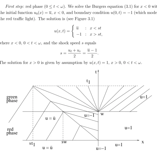
In the following, we will consider the Lighthill-Whitham-Richards model in some de- tail. More precisely, we want to study the influence of a temporal disturbance due to a traffic interruption (for instance, a traffic light). Suppose that the highway is initially filled with cars with uniform density ρ in the interval (−∞,0), that there is a red light atx= 0, and that the highway is empty in (0,∞). We work with the transformed equa- tion (3.1) and the uniform density u = 1−2ρ/ρmax. Clearly, there will be a tailback in front of the traffic light. At time t = ω, the traffic light changes from red to green, and
the cars move from the left to the right. We want to know what happens with the tailback at timet > ω.
First step: red phase (0≤t < ω). We solve the Burgers equation (3.1) for x <0 with the initial functionu0(x) = u,x <0, and boundary conditionu(0, t) = −1 (which models the red traffic light). The solution is (see Figure 3.1)
u(x, t) =
( u : x < st
−1 : x > st, where x <0, 0 < t < ω, and the shock speeds equals
s= u`+ur
2 = u−1 2 .
The solution for x >0 is given by assumption byu(x, t) = 1, x >0, 0< t < ω.
t1
u = u
u = u
s x
u=−1 u=1 u=1
u=1
u=−1 w
sw green
red phase
phase
t1 t
Figure 3.1: Characteristics for the traffic flow problem.
Second step: green phase (t ≥ ω). We solve the Burgers equation (3.1) in R, with initial datum u0(x) = u(x, ω). Since u` = u > −1 = ur we get a shock ψ(t) = st, t > ω, with speed s = (u−1)/2 < 0. A rarefaction wave develops at x = 0, since u` =−1<1 =ur. The solution is given by
u(x, t) =
u : x < st,
−1 : st≤x < ω−t,
x
t−ω : ω−t≤x≤t−ω, 1 : x > t−ω,
x∈ R, t > ω. This solution makes sense as long as st < ω−t or, equivalently, t < t1 :=
ω/(s+ 1) = 2ω/(u+ 1).
Third step: green phase (t > t1). What happens with the shock fort > t1? The shock speed is given by the generalized Ranking-Hugoniot condition (2.7):
s(t) = ψ0(t) = 1
2(u(ψ(t) + 0, t) +u(ψ(t)−0, t))
= 1
2
µψ(t) t−ω +u
, t > t1. This is a linear ordinary differential equation with inital condition
ψ(t1) =st1 =ωu−1 u+ 1. The solution is
ψ(t) = u(t−ω)−√ t−ω
q
ω(1−u2), t≥t1.
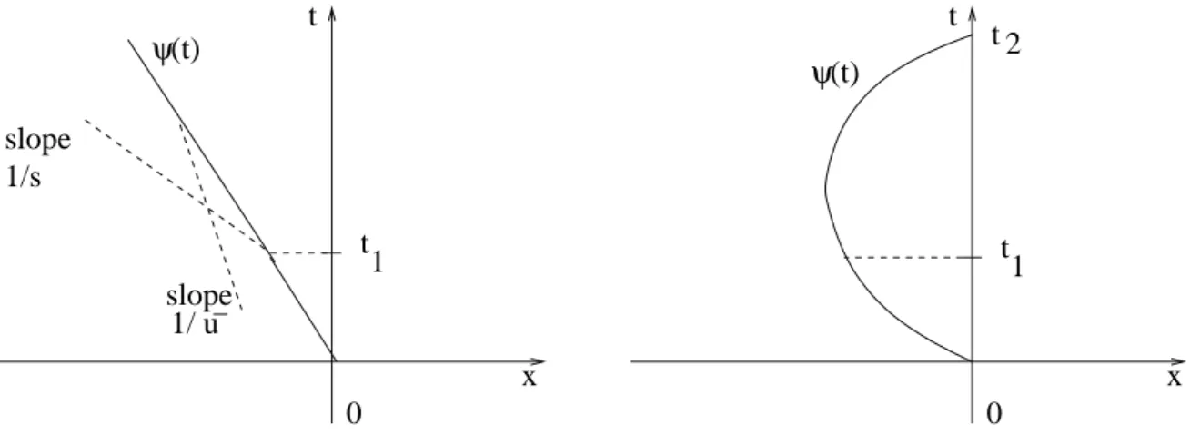
Now there are two cases. If u ≤ 0, ψ(t) → −∞ as t → ∞, i.e., there is a shock for all time and the shock moves into the negative x-direction with shock speed ψ0(t) → u (t → ∞). The velocity of the shock line is thus reduced from s = (u−1)/2 to u ≥ s.
Clearly, the discontinuity step at ψ(t) goes to zero as t → ∞. However, the drivers observe the shock even a long time after the traffic disturbance. This agrees with practical experience.
ψ(t)
ψ(t)
slope
t t
t 2
0 0
t t
x x
slope 1/s
1/ u
1 1
Figure 3.2: Shock curve ψ(t) foru≤0 (left) and u >0 (right).
In the other case, u > 0, ψ(t) → ∞ as t → ∞, i.e., the shock line moves into the positive x-direction. Suppose that after the time t = 2ω the traffic light changes from green to red. How long should the green phase be to eliminate the shock, i.e., we need t2 ≤ 2ω where ψ(t2) = 0. The equation ψ(t2) = 0 has the (unique) solution t2 = ω/u2.
Thus, t2 ≤2ωis satisfied if and only if u≥1/√
2. The tailback in front of the traffic light will vanish during the green phase if and only ifu≥1/√
2 or, in original density, ρ≤ρ0 := ρmax
2 µ
1− 1
√2
≈0.146ρmax,
independently of the length of the green phase! Even for moderate vehicle densityρ > ρ0, the tailback in front of the traffic light will become larger and larger as time increases.
4 Numerical approximation of scalar conservation laws
Before studying numerical methods for nonlinear scalar equations we start with a very simple linear equation:
ut+aux = 0, x∈R, t >0, (4.1)
u(x,0) = u0(x), x∈R, (4.2)
wherea >0. This problems has the explicit solution u(x, t) =u0(x−at) which is a weak solution (at least if u0 is “smooth” enough).
We discretize the (x, t)-plane by the mesh (xi, tn) with xi =ih (i∈Z), tn=nk (n ∈N0)
andh, k >0. For simplicity of presentation we take a uniform mesh withhandkconstant, but the discussed methods can be easily extended to non-uniform meshes. We are looking for finite difference approximations uni to the solutionu(xi, tn) at the discrete grid points.
The idea is to replace the partial derivatives in (4.1) by difference quotients. For example, (4.1) can be written by Taylor expansion as
u(xi, tn+1)−u(xi, tn)
k +O(k) =−a u(xi+1)−u(xi−1)
2h +O(h2), (4.3)
which motivates the first numerical scheme:
Central scheme: Consider the approximation of (4.3) un+1i −uni
k =−a uni+1−uni−1
2h , n ≥0, i∈Z. We can write this scheme as
un+1i =uni − ak
2h (uni+1−uni−1). (4.4)
As we can compute un+1i from the data uni explicitely, this is anexplicitscheme. Another idea would be to use the scheme
un+1i −uni
k =−a un+1i+1 −un+1i−1 2h or, equivalently,
ak
2hun+1i+1 +un+1i − ak
2hun+1i−1 =uni.
This is an implicit scheme. In each time step, a linear system has to be solved. As for time-dependent hyerbolic equations, implicit schemes are rarely used, we consider in the following only explicit schemes.
In practice we must compute on a finite spatial domain, say 0 ≤ x ≤ N h, and we require appropriate boundary conditions at x = 0, x = N h, respectively. For the above equation we choose periodic boundary conditions
u(0, t) =u(N h, t), t >0, or, for the approximations uni,
un0 =unN, n≥0.
We can determine un0 and unN using (4.4). In fact, setting i = 0 or i = N in (4.4) would require to determineun−1 orunN+1, We consider these points as artificial points with un−1 = unN−1 and unN = uN0 , by the periodicity. Therefore, our central scheme reads as follows
u0i = u0(xi), i= 0, . . . , N, un+1i = uni −ak
2h(uni+1−uni−1), i= 1, . . . , N −1, un+10 = un0 −ak
2h(un1 −unN−1), un+1N = unN − ak
2h(un1 −unN−1).
Thus, if un0 = unN then un+10 = un+1N , and the periodicity is preserved. This scheme has the advantage that it is mass-preserving, i.e.
N−1X
i=0
uni =
N−1X
i=0
u0(xi), n ≥0.
Indeed,
N−1X
i=0
un+1i =
N−1X
i=1
·
uni − ak
2h(uni+1−uni−1)
¸
+un0 − ak
2h(un1 −unN−1)
=
N−1X
i=0
uni − ak 2h
ÃN−1 X
i=0
uni+1− XN
i=1
uni−1
!
= XN
i=0
uni − ak
2h(unN −un0)
= XN
i=0
uni.
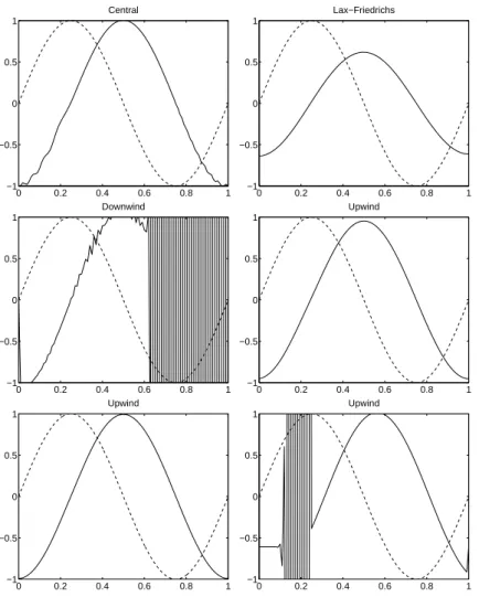
Figure 4.1 (first row, left) shows the numerical solution using the above central scheme for a= 1, h= 0.01, N = 100,k = 0.001, with initial data
u0(x) = sin(2πx), 0≤x≤1, (4.5)
at time t = 0 (broken line) and t = 0.25 (solid line). The result is an approximation of sin(2π(x−0.25)). We see that the solution is oscillating. This can be improved by using an arithemetic average in the approximation of the time derivative and leads to the following scheme.
Lax-Friedrichs scheme. In this scheme the time derivative is approximated by 1
k µ
u(x, t+k)− 1
2(u(x+h, t) +u(x−h, t))
¶ , i.e.
un+1i = 1
2(uni+1+uni−1)− ak
2h(uni+1−uni−1), i= 1, . . . , N −1. (4.6) The initial and boundary data are approximated by the same idea as for the central scheme. It is not difficult to check that the Lax-Friedrichs scheme is mass-preserving.
Its numerical solution in Figure 4.1 (first row, right) with the same parameters as above shows that there are no oscillations, but now the solution is too smeared out. What happened?
We use the exact solution in the scheme (4.6) to compute the so-called truncation error
T E(x, t) = 1 k
µ
u(x, t+k)− 1
2(u(x+h, t) +u(x−h, t))
¶ + a
2h(u(x+h, t)−u(x−h, t)).
0 0.2 0.4 0.6 0.8 1
−1
−0.5 0 0.5 1
Central
0 0.2 0.4 0.6 0.8 1
−1
−0.5 0 0.5 1
Lax−Friedrichs
0 0.2 0.4 0.6 0.8 1
−1
−0.5 0 0.5 1
Downwind
0 0.2 0.4 0.6 0.8 1
−1
−0.5 0 0.5 1
Upwind
0 0.2 0.4 0.6 0.8 1
−1
−0.5 0 0.5 1
Upwind
0 0.2 0.4 0.6 0.8 1
−1
−0.5 0 0.5 1
Upwind
Figure 4.1: Various numerical schemes for (4.1) with a = 1, h = 0.01, k = 0.001 and smooth initial data (4.5). The numerical solution fort= 0 (broken line) andt= 0.25 (solid line) is shown. First row: central (left), Lax-Friedrichs (right); second row: downwind (left), upwind (right); last row: upwind but with h= 0.002 (left) and k= 0.0025 (right).
A Taylor expansion yields at (x, t) T E = 1
k
·µ
u+utk+1
2uttk2+O(k3)
−1 2
¡2u+uxxh2+O(h4)¢¸ + a
2h(2uxh+O(h3))
= ut+aux+1 2
µ
uttk−uxx
h2 k
+O(k2) +O³h4 k
´+O(h2).
Since utt =−auxt=a2uxx and assuming thatk/h= const., we conclude T E(x, t) = k
2
³a2−³h k
´2´
uxx(x, t) +O(h2) =O(k). (4.7)
This shows first that the Lax-Friedrichs scheme is a first-order method (as the truncation error satisfies |T E(x, t)| ≤ Ck for all (x, t)) and second that we approximate up to an error of the form kuxx. Now, spatial second derivatives are modeling diffusion phenom- ena, and we expect the discrete solutions to be smeared out—justified by the numerical experiments. The numerical solution generated by the Lax-Friedrichs scheme can serve as an approximation of the advection-diffusion equation
ut+aux =−k 2
³a2−³h k
´2´
uxx, x∈R, t >0.
Forh→0 andk →0, the solutions of this modified equation converge (at least formally) to the solution of ut+aux = 0. This is related to the vanishing viscosity limit discussed in Section 3. The Lax-Friedrichs approximation becomes better and better for smaller k >0. Moreover, theartificial diffusion (also called artificial viscosity) avoids oscillations.
Downwind scheme. The Lax-Friedrichs scheme gives accurate approximations only if k (or, equivalently, h if k/h= const.) is sufficiently small. One-sided finite difference ap- proximations avoid too much artificial diffusion. Therefore, we choose the approximation
un+1i =uni −ak
h (uni+1−uni), i= 0, . . . , N −1,
with initial and periodic boundary conditions analogously as above. Also this scheme is mass-preserving. The numerical solution shows that the scheme is unstable (Figure 4.1 (second row, left); same parameters as above). Why? The solution describes a “wave”
from the left to the right. The spatial derivative at xi, however, uses the information at xi+1 where the “wave” will go in the next time step. This does not make sense. In fact, the above scheme is useless. It would be more reasonable to use the information at xi−1
where the “wave” comes from. This is done in the following scheme.
Upwind scheme. This scheme reads as follows un+1i =uni − ak
h (uni −uni−1), i= 1, . . . , N. (4.8) Again, the scheme is mass-preserving. Its numerical solution with the same parameter values as in the previous schemes in Figure 4.1 (second row, right) shows the correct solution, no oscillations, but with artificial diffusion. In fact, the truncation error
T E(x, t) = 1
k(u(x, t+k)−u(x, t)) + a
h(u(x, t)−u(x−h, t)) can be written as
T E(x, t) = ak 2
³a− h k
´uxx +O(h2) +O(k2). (4.9)
The corresponding equation with artificial diffusion reads here:
ut+aux =−ah 2
³ a− h
k
´
uxx. (4.10)
For the values of a, k and h used here, the diffusion term is 0.0045uxx, whereas the cor- responding term in the Lax-Friedrich scheme is 0.0495uxx. Thus, we expect upwind to be less diffusive than Lax-Friedrichs, as confirmed by the numerical experiments. Choos- ing h > 0 smaller, the diffusion becomes less apparent and for h = 0.002 the numerical solution is close to the exact solution (Figure 4.1 (last row, left)).
For small k > 0, we need a lot of time steps to compute the solution at a certain fixed time. Can we accelerate the computations by choosing k larger? Figure 4.1 (last row, right) shows the result for h= 0.01 and k = 0.0025 (a and u0 are as above). Thus, the answer is no. Why? The modified equation (4.10) is well-posed only if the diffusion coefficient is non-negative:
−ah 2
³ a− h
k
´
≥0 ⇐⇒ ak
h ≤1. (4.11)
In the converse case we do not have diffusion but concentration. In the above situation we have ak/h = 2.5 > 1, and we expect the solution to break down after some time.
The condition (4.11) is known as the Courant-Friedrich-Levy (CFL) condition. Strictly speaking, the CFL condition is not defined by (4.11) but equivalent to it, and we will identify the CFL condition and (4.11). This condition imposes a severe restriction on the choice of the time step; the more accurate the solution is computed (we mean: h > 0 small), the smaller k > 0 has to be chosen and the longer the computations take.
In Figure 4.2 we illustrate the described behavior using discontinuous initial data u0(x) =
( 1 : 0 ≤x <1/2
0 : 1/2≤x≤1 (4.12)
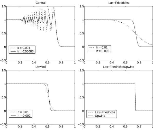
and the parameters a= 1, t = 0.25, k = 0.001. We restrict the computational domain to [0,1]. We do not choose periodic boundary conditions here, but inflow- and outflow-type conditions. In the traffic flow interpretation, the traffic is heavy in [0,1/2) and light in [1/2,1]. So, at x = 0, cars are entering the domain and are leaving at x = 1. Hence, in the discrete formulation,
un+11 =un0 and un+1N =unN−1, n≥0. (4.13) We observe again that the central scheme is oscillatory with damped oscillations for smaller k (Figure 4.2 (first row, left); h = 0.01); the Lax-Friedrichs scheme is quite diffusive but not oscillatory (Figure 4.2 (first row, right)); and the upwind scheme is less diffusive than the Lax-Friedrichs scheme (Figure 4.2 (last row, left)). Choosing the mesh
0 0.2 0.4 0.6 0.8 1
−0.5 0 0.5 1 1.5
Central
k = 0.001 k = 0.00005
0 0.2 0.4 0.6 0.8 1
−0.5 0 0.5 1 1.5
Lax−Friedrichs
h = 0.01 h = 0.002
0 0.2 0.4 0.6 0.8 1
−0.5 0 0.5 1 1.5
Upwind
h = 0.01 h = 0.002
0 0.2 0.4 0.6 0.8 1
−0.5 0 0.5 1 1.5
Lax−Friedrichs/Upwind
Lax−Friedrichs Upwind
Figure 4.2: Various numerical schemes for (4.1) with a= 1 and discontinous data (4.12).
First row, left: central; first row, right: Lax-Friedrichs; last row, left: upwind; last row, right: Lax-Friedrichs (broken line) and upwind (solid line) for h= 0.001, k = 0.001.
size h = k = 0.01, both schemes produce a solution which is very close to the exact solution (Figure 4.2 (last row, right)). This is clear since for this choice, a−h/k = 0 holds and thus, the artificial diffusion in (4.7) and (4.9) vanishes. All these schemes are able to compute the correct shock speed.
Summarizing the above results we observe that the central scheme tends to produce oscillations whereas the other diffusive schemes have usually too much artificial viscosity except for special mesh sizes.
The traffic flow models are nonlinear, so we want to study what can happen when we discretize nonlinear equations. We choose the scaled Lighthill-Whitham-Richards model (which is the same as the inviscid Burgers equation)
ut+uux = 0, x∈R, t >0, (4.14)
u(x,0) = u0(x), x∈R, (4.15)
with initial data (4.12). A “natural” generalization of the linear upwind scheme could be un+1i =uni − k
huni(uni −uni−1), t∈Z, n ≥0.
Since u0i = 0 if i ≥ N/2 and u0i −u0i−1 = 0 for i < N/2, u1i = u0i for all i. This happens in every time step and so uni =u0i for all i. As the grid is refined, the numerical solution converges to the function u(x, t) =u0(x). This is not a weak solution of (4.14)–(4.15)!
One might think that the upwind scheme un+1i =uni −k
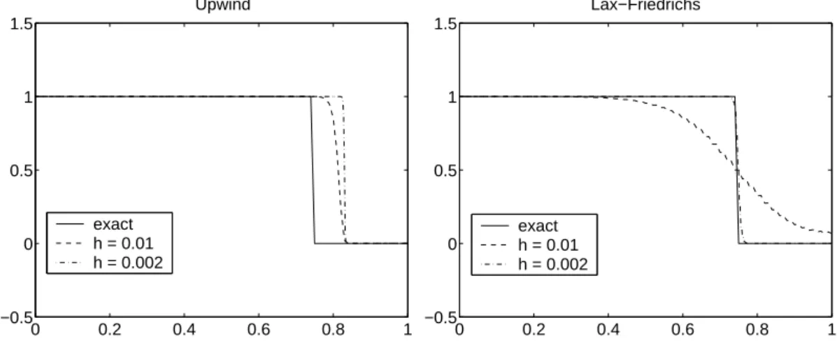
huni−1(uni −uni−1), i∈Z, n≥0, (4.16) gives better results since here we use the information from the left where the “wave” is coming from. The numerical solution of this scheme (with boundary conditions (4.13) and k = 0.001, t = 0.5) is depicted in Figure 4.3 (left). For smaller mesh size, the numerical solution converges nicely to a function of type u0(x−at). The exact solution of (4.14)–(4.15), (4.12) is
u(x, t) =
( 1 : x < st 0 : x > st
with s = 12(u` +ur) = 12. At t = 12, the discontinuity should be at x = 34. Thus, the numerical solution propagates with the wrong speed!
0 0.2 0.4 0.6 0.8 1
−0.5 0 0.5 1 1.5
Upwind
exact h = 0.01 h = 0.002
0 0.2 0.4 0.6 0.8 1
−0.5 0 0.5 1 1.5
Lax−Friedrichs
exact h = 0.01 h = 0.002
Figure 4.3: Exact and numerical solutions for the inviscid Burger equation using the upwind scheme (4.16) (left) and the Lax-Friedrichs scheme (4.17) (right).
A better behavior is given by the Lax-Friedrichs scheme un+1i = 1
2(uni+1+uni−1)− k 4h
¡(uni+1)2−(uni−1)2¢
, i∈Z, n ≥0. (4.17)
From Figure 4.3 (right) we see that the scheme is non-oscillatory and the shock speed is correct.
What is the reason for the different shock speeds? The upwind scheme (4.16) is a discretization of the quasilinear equation
ut+uux = 0,
whereas the scheme (4.17) is an approximation of the equation in conservation form ut+
µu2 2
x
= 0.
For smooth solutions both equations are the same, but we know from Section 2 (see, for instance, Example 2.8) that this may not be true for weak solutions.
In the following we consider only numerical methods being inconservation form, mean- ing that the scheme is of the form
un+1i =uni − k
h[F(uni−p, . . . , uni+q)−F(uni−1−p, . . . , uni−1+q)]
for some functionF of p+q+ 1 arguments. We call F the numerical flux function. The simplest case is for p= 0 andq = 1, where
un+1i =uni − k
h[F(uni, uni+1)−F(uni−1, uni)]. (4.18) This expression can be interpreted as a cell average. More precisely, we know that the weak solution of
ut+f(u)x = 0, x∈R, t >0, (4.19) satisfies the integral form
1 h
Z xi+1/2
xi−1/2
u(x, tn+1)dx = 1 h
Z xi+1/2
xi−1/2
u(x, tn)dx (4.20)
− k h
·1 k
Z tn+1
tn
f(u(xi+1/2, t))dt− 1 k
Z tn+1
tn
f(u(xi−1/2, t))dt
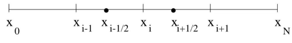
¸ , where xi±1/2 = (i±1/2)h denotes the cell middle points (see Figure 4.4). Interpretating uni as approximations of the cell averages,
uni ∼ 1 h
Z xi+1/2
xi−1/2
u(x, tn)dx,
andF(uni, uni+1) as approximations of the average flux throughxi+1/2over the time interval (tn, tn+1),
F(uni, uni+1)∼ 1 k
Z tn+1
tn
f(u(xi+1/2, t))dt, we obtain the approximation (4.18) from (4.20).
We give now some examples of numerical methods in conservation form:
x x x x x x
0 i-1 i-1/2 i i+1 N
. .
x
i+1/2Figure 4.4: The spatial mesh.
Example 4.1
(1) Lax-Friedrichs scheme:
un+1i = 1
2(uni+1+uni−1)− k
2h(f(uni+1)−f(uni−1)).
This method can be written in the conservation form (4.18) by taking F(uni, uni+1) = h
2k(ui−ui+1) + 1
2(f(ui) +f(ui+1)).
It can be proved that this scheme is a first-order method (i.e., the truncation error T E satisfies|T E|=O(k) as k →0).
(2) Lax-Wendroff scheme:
un+1i = uni − k
2h(f(uni+1)−f(uni−1)) + k2
2h2[f0(uni+1/2)(f(uni+1)−f(uni))−f0(uni−1/2)(f(uni)−f(uni−1))], whereuni±1/2 = 12(uni +uni±1/2). This is a second-order method (i.e. |T E|=O(k2) as k →0). It has the disadvantage that it requires evaluating f0 in two points at each time step which is expensive when we deal with systems of conservation laws (and f0 is the Jacobi matrix). This is avoided in the following schemes.
(3) Richtmyer two-step Lax-Wendroff scheme:
u∗i = 1
2(uni +uni+1)− k
h[f(uni+1)−f(uni)], un+1i = uni − k
h[f(u∗i)−f(u∗i−1)].
This is a second-order method. Notice that the derivation of the local truncation error T E(x, t) needs smooth solutions, so all these second-order methods are of second order for smooth solutions. The methods are usually only of first order around shocks.
(4) Mac-Cornack scheme:
u∗i = uni −k
h[f(uni+1)−f(uni)], un+1i = 1
2(uni +u∗i)− k
h[f(u∗i)−f(u∗i−1)].
This scheme uses first forward differencing and then backward differencing. It is also a second-order method. Notice that the schemes (2)–(4) reduce to the Lax-Wendroff method if f is linear.
All the described schemes in Example 4.1 yield numerical solutions which converge to a weak solution of (4.19) if the mesh discretization parameters h and k tend to zero. In order to formulate this result more generally we need the following definitions. From now on, we assume that f :Rn →Rn is a vector-valued function, i.e., we considersystems of conservation laws (4.19).
Definition 4.2 (1) A difference scheme of the form un+1i =uni − k
h[F(uni−p, . . . , uni+q)−F(uni−1−p, . . . , uni−1+q)]
for some function F : (Rn)p+q+1 →Rn is called conservative.
(2) A conservative scheme is called consistent if F is locally Lipschitz continuous and F(u, . . . , u) = f(u) ∀u∈R.
(3) The total variation T V(v) of a function v :R→Rn is defined by T V(v) = sup
XN
i=1
|v(ξi)−v(ξi−1)|,
where the supremum is taken over all subdivisions −∞= ξ0 < ξ1 < . . . < ξn =∞ of the real line.
Notice that for the total variation to be finitevmust approach constant values asx→ ±∞. For differentiable v the definition reduces to
T V(v) = Z
R|v0(x)|dx.
Theorem 4.3 (Lax-Wendroff) Let uj(x, t) be a numerical solution computed with a con- sistent and conservative method on a mesh with mesh size hj and time step kj, with hj, kj →0 as j → ∞. (The function uj can be, for instance, the constant extension of uni in the cells.) Assume that there exists a function u(x, t) such that
(1) for all a, b∈R, T >0, Z T
0
Z b
a |uj(x, t)−u(x, t)|dxdt→0 asj → ∞, (2) for all T >0 there is a number K >0 such that
T V(uj(·, t))≤K ∀0≤t ≤T, j∈N. Then u(x, t) is a weak solution of (4.19).
For the proof we refer to [5, Sec. 12]. Theorem 4.3 does not guarantee that weak solutions obtained in this way satisfy the entropy condition. This is true under the following additional condition.
Theorem 4.4 Let (η, ψ) be an entropy-entropy flux pair such that η00(u) > 0 and η0(u) divf(u) = divψ(u) for all u ∈ Rn. Furthermore, let Ψ be a numerical flux function consistent with ψ in the sense of Definition 4.2 (2). Let the assumptions of Theorem 4.3 hold and, additionally,
η(un+1i )≤η(uni)− k
h[Ψ(uni−p, . . . , uni+q)−Ψ(uni−1−p, . . . , uni−1+q)]
for all i, n. Thenu(x, t) (obtained in Theorem 4.3) satisfies the entropy inequality (2.13).
Again, we refer to [5, Sec. 12] for a proof.
5 The Gudonov method
In Section 4 we have seen that a nonlinear conservation law (or a system of conservation laws) can be numerically approximated by the Lax-Friedrichs scheme. For the linear advection equation (4.1) we have also seen that the Lax-Friedrichs scheme is generally more dissipative than the upwind method and gives less accurate solutions. In the scalar case, a natural generalization of the upwind scheme (4.8) is
un+1i =uni − k
h[F(uni, uni+1)−F(uni−1, uni)] (5.1) with
F(v, w) =
( f(v) : (f(v)−f(w))/(v−w)≥0 f(w) : (f(v)−f(w))/(v−w)<0.