Volatility forecasting accuracy for Bitcoin

SFB 823

Volatility forecasting accuracy for Bitcoin

Discussion Paper Gerrit Köchling, Philipp Schmidtke,

Peter N. Posch

Nr. 14/2019

Volatility Forecasting Accuracy for Bitcoin

Gerrit K¨ ochling ^∗ , Philipp Schmidtke ^† , Peter N. Posch ^‡ July 1, 2019

Abstract

We analyse the quality of Bitcoin volatility forecasting of GARCH-type models applying the commonly used volatility proxy based on squared daily returns as well as a jump-robust proxy based on intra-day returns and vary the degrees of asymmetry in robust loss functions. We construct model confidence sets (MCS) which contain superior models with a high probability and find them to be systematically smaller for asymmetric loss functions and the jump robust proxy. Our findings suggest a cautious use of GARCH models in forecasting Bitcoin’s volatility.

Keywords: Bitcoin, Cryptocurrency, GARCH, Volatility, Model Confidence Set, Robust loss function

JEL classification: C5, C22, G1

Acknowledgements: We would like to thank the German Research Foundation (DFG) for financial support by the Collaborative Research Center “Statistical

∗

TU Dortmund University, Chair of Finance, Otto-Hahn-Str. 6, 44227 Dortmund, Germany.

email: gerrit.koechling@udo.edu. Corresponding author.

†

see above. email: philipp.schmidtke@udo.edu.

‡

see above. email: peter.posch@udo.edu.

modeling of nonlinear dynamic processes” (SFB 823). Furthermore, we would like

to thank the organizer and participants of the Cryptocurrency Research Confer-

ence 2019, Southampton for valuable input. We claim full responsibility for all

remaining errors.

1 Introduction

Time-series modeling of cryptocurrencies’ returns has recently gained increased at- tention. As for many traditional assets, the inter-temporal dependence of volatil- ity is of special interest. GARCH-type models were the first to be applied, cf.

Dyhrberg (2016), who models returns on Bitcoins with a standard GARCH(1,1) model as well as an E-GARCH(1,1) model to detect similarities with gold and the US-Dollar. Katsiampa (2017) focuses on in-sample estimates of six GARCH mod- els and adds the question of model choice to the literature, which Chu et al. (2017) extends to seven cryptocurrencies fitted with twelve GARCH models. Recently, Troster et al. (2018) perform model comparison analysis with many GARCH mod- els using in-sample criteria and backtests of Value-at-Risk forecasts.

We focus on the out-of-sample forecasting of return volatility using the classical volatility proxy based on squared daily returns as well as a robust alternative based on 30 minutes intra-day returns. We evaluate the 1-day ahead volatility forecasts using 172 GARCH-type models and three robust loss functions with different degrees of asymmetry. Finally, we construct model confidence sets as introduced by Hansen et al. (2011) to allow for statistically sound differentiation between equal-performing and underperforming models.

We find evidence that our jump-robust volatility proxy based on intra-day re-

turns and asymmetric loss functions, e.g. functions that penalize overestimation

of volatility less than underestimation, perform better. However, the model confi-

dence sets are rather large, implying that no family of models or any single model

outperforms. Out of all tested specifications we identify a set of 88 models which

are never outperformed. Regarding the conditional density of the innovations,

Gaussian distributions tend to remain more often within the model confidence set

than t-conditional distributions. For mean-modeling and GARCH orders, we find

only small differences. We thus conclude with the caveat that there does not seem

to exist a ’one-fits-all’ type of model and thus adequate Bitcoin volatility forecast- ing needs a close look at the specification in order to obtain a strong model.

2 Methodology

In this section we introduce the techniques of forecast evaluation which we use to assess the forecasts of the models described in the following section.

Volatility Proxies Due to the latent nature of the conditional variance σ

of the financial return r

, it is common to use ex-post estimators denoted proxies. We use the square of the daily return r

which can be interpreted as the sample variance consisting only of one observation r

while assuming a zero mean for r

. Since this estimator is known to be noisy (Andersen and Bollerslev (1998)) several authors, eg. Andersen et al. (2001) or Barndorff-Nielsen and Shephard (2002) propose high- frequency data as an alternative source to proxy volatility. The trading day t is divided into m equally sized sub-periods with return r

in sub-period i. Assuming a simple data generating process, realized volatility/variance RV

is the sum of squared intra-day returns and can be written as RV

= P

i=1

r

. This estimator, however, is not robust to jumps, which are often present in intra-day data. A jump robust realized volatility estimator is introduced by Andersen et al. (2012) as

MedRV = π

6 − 4 √ 3 + π

m m − 2

X

i=2

median(|r

|, |r

|, |r

|)

and applied here.

Loss Functions To evaluate the performance of the volatility forecasts we em- ploy the following family of robust and homogeneous loss functions:

L(ˆ σ

, h; b) =



 

 

 

 

 

 

1

(b+1)(b+2)

σ ˆ

− h

−

h

(ˆ σ

− h) for b / ∈ {−1, −2}, h − σ ˆ

+ ˆ σ

log(

) for b = −1,

ˆ σ²

h

− log(

) − 1 for b = −2,

(L) where ˆ σ is the volatility forecast, h the volatility proxy and b a parameter deter- mining the shape of the function. Patton (2011) shows these functions to select the true volatility even if noise in the proxy is present. Up to multiplicative and additive constants, the mean squared error (MSE) loss function obtains for b = 0.

For values of b below zero (L) penalizes underestimation of volatility heavier than overestimation which can be interesting for risk management purposes. Beside b = 0, we hence include the cases b = −1 (MIX) and b = −2, which corresponds to the QLIKE loss function.

Testing Losses To test for significant differences in the performance of the models we employ model confidence sets as introduced by Hansen et al. (2011).

This concept is related to tests for comparing forecasts (Diebold and Mariano, 1995; West, 1996) but addresses data snooping which is important since the number of potential models is large. MCS improve earlier techniques controlling for data snooping like White (2000)’s reality check and the test for superior predictive ability by Hansen (2005).

The MCS procedure does not rely on a benchmark model but starts at the

full universe of models and iteratively drops models by alternately applying a test

of equal predictive ability at significance level α and an elimination rule. The

algorithm delivers a set of eliminated models which are significantly inferior to the

models remaining in the MCS which have statistically equal predictive ability. The MCS contains the true set of superior models with high probability 1 − α similar to a confidence interval.

3 Empirical Analysis and Results

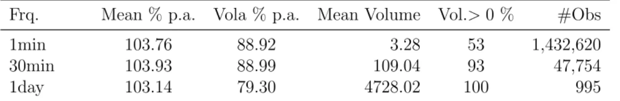
Data We obtain Bitcoin-USD exchange rate data at the 1-minute frequency from the crypto exchange Gemini which is one of the largest crypto exchanges and its prices also served as the basis for the daily settlement of the Bitcoin futures of the Chicago Board Option Exchange CBOE. We restrict the data to the period from 2015-11-30 to 2018-08-20 where no observations are missing to construct 30-minute and daily time-series. Table 1 presents descriptive statistics.

Frq. Mean % p.a. Vola % p.a. Mean Volume Vol.> 0 % #Obs

1min 103.76 88.92 3.28 53 1,432,620

30min 103.93 88.99 109.04 93 47,754

1day 103.14 79.30 4728.02 100 995

Table 1: Descriptive statistics of log returns and volume data from the Gemini exchange from 2015-11-30 to 2018-08-20.

Table 1 shows the high returns and high volatility of Bitcoin during our sample period. The market’s activity, measured by the percentage of positive volume, is relatively small for the 1-minute periods (53 %) but trading activity picks up when the interval is extended to the 30-minute frequency, which provides a meaningful trade-off between high frequency and trading activity.

Forecasting with GARCH Models We combine two specifications for the

conditional mean (zero and ARMA(1,1) denoted as µ

and µ

, respectively), eleven

models for the conditional variance

with orders p, q ∈ {1, 2}, and two conditional distributions (Gaussian N and Student t-distribution) to obtain 172 models in to- tal.

We calculate one-day-ahead volatility forecasts by applying a rolling-window scheme with slightly more than one year of log-returns. The first out-of-sample day is 2017-01-01, the whole out-of-sample period covers 597 days. The models are refitted every five returns. After the estimation process, we drop models with invalid forecast values (NaN) and continue with 148 models as input for the MCS construction procedure.

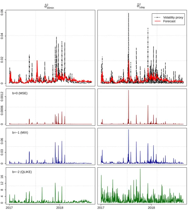
Figure 1 presents the time-series of forecasts and proxies as well as the three loss functions. It shows the intra-day proxy to be less volatile. Especially for the turn of the year period 2017/2018, the intra-day proxy indicates return volatility more precisely which inherits from the loss functions where losses for the intra- day proxy are dominated by this period. In addition, the plots illustrate how differently the loss functions assess deviations. MSE tends to be more prone to extreme judgements whereas QLIKE losses are more centered.

1

ARCH, GARCH, IGARCH, E-GARCH, GJR-GARCH, APARCH, CS-GARCH, AVGARCH, TGARCH, NGARCH and NAGARCH as specified in Ghalanos (2017).

2

For ARCH specifications we include p ∈ {1, 2, 3}.

00.020.040.06

σ^

30min

2 σ^

1day 2

Volatility proxy Forecast

b=0 (MSE)

00.00060.0012

b=−1 (MIX)

00.030.06

2017 2018

mod_min30_qlike2

b=−2 (QLIKE)

0481216

2017 2018

mod_min1day_qlike2

Figure 1: Comparison of standard GARCH(1,1), N, µ

1-day ahead volatility

forecasts using squared daily returns (right) and the jump robust sum of squared

30-minute returns (left) as volatility proxies. Upper charts show the volatility

proxy (black dotted) and the forecast (red solid). The charts below show the

corresponding losses for b ∈ {0, −1, −2} (top to bottom).

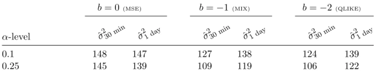
Model confidence sets For each combination of significance level α ∈ {0.10, 0.25}, loss function parameter b ∈ {0, −1, −2}, and volatility proxy ˆ σ

, i ∈ {30 min, 1 day}, we construct a model confidence set. The numbers of models with equal predic- tive ability are presented in Table 2. We find evidence that both asymmetric loss functions and the volatility proxy based on intra-day returns systematically allow for more rejections.

Table 3a shows the specifications which were most frequently dropped. We find relatively sophisticated models within this group which are all endowed with a conditional t-distribution. Table 3b confirms this tendency as the majority of models kept in the MCS are endowed with a Gaussian distribution. Regarding the maximum order of the models we do not find substantial differences. It seems that mean modeling is also rather negligible.

Overall, 88 models remain in the inter- section of all MCS suggesting that finding one outperforming model is a challenge.

Only the IGARCH model family remain in all MCS recommending themselves as a promising choice.

b = 0

b = −1

b = −2

α-level σ ˆ

σ ˆ

y

ˆ σ

σ ˆ

y

σ ˆ

σ ˆ

0.1 148 147 127 138 124 139

0.25 145 139 109 119 106 122

Table 2: Number of superior models contained in the MCS in each setting.

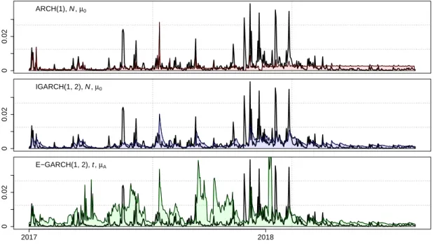
We proceed by studying Figure 2 which depicts forecasts and proxies for two models which have never been dropped from any MCS and one of the worst during

3

Note that the percentages in Table 3b denote the proportion of applicable models with the

same property.

Model # Dropped E-GARCH(1,2), t, µ

9 E-GARCH(2,1), t, µ

8 T-GARCH(1,2), t, µ

8 T-GARCH(2,2), t, µ

7

ARCH(3), t, µ

7

APARCH(1,1), t, µ

6

APARCH(2,1), t, µ

6

E-GARCH(2,2), t, µ

6 T-GARCH(1,1), t, µ

6 T-GARCH(1,1), t, µ

6

(a) Most frequently dropped models.

Property # Perc.

Panel A: Cond. distributions

N 58 77.33

t 30 41.10

Panel B: Mean models

µ

46 60.53

µ

42 58.33

Panel C: GARCH orders

(1, 1) 23 63.89

(∗, 0) 1 8.33

(2, 2), (1, 2), (2, 1) 64 64.00 (b) Characteristics of models which remain in all MCS.

Table 3: Models which were most frequently dropped from or contained in MCS.

The maximum number is determined by the number of scenarios.

the MCS procedure.

However, the forecasts exhibit fundamentally different tem- poral features. The ARCH(1) forecasts are relatively stable whereas the forecasts of IGARCH(1,2) vary substantially. Although the latter model seems to be more reactive and is visually better in capturing the variance fluctuations, the time to cool down after high volatility is long compared to the proxy. The forecasts of the underperforming E-GARCH(1,2) model in the bottom plot are highly active as well but tend to overpredict the volatility over long periods.

Although we detect some steadily outperforming models across our settings, the fact that a simple ARCH(1) performs comparatively well indicates that even sophisticated models can have problems to get along with the Bitcoin dynamics.

4

The mean loss of the ARCH(1), N , µ

model is 1.01, that of the IGARCH(1,2), N , µ

model

is 0.83. As revealed by the MCS procedure both losses are significantly smaller than that of

the E-GARCH(1,2), t, µ

model with 3.48 in most settings. Note that the mentioned numbers

belong to the 30 min proxy with b = 0 (MSE) loss function and are scaled by 10

.

00.02

ARCH(1), N , µ0

00.02

IGARCH(1, 2), N , µ0

2017 2018

00.02

E−GARCH(1, 2), t , µA

Figure 2: Forecasts of two models which have not been dropped from any MCS (top) and one of the worst models (bottom) during the MCS procedure. Black solid line shows the volatility proxy based on 30 minute returns.

4 Conclusion

Choosing a single GARCH-like model as an unequivocally well forecasting tool is a challenging task since the sizes of model sets with equal predictive ability are relatively large. However, we do find some model specifications which tend to be outperformed on a regular basis. While conditional mean modeling is rather negligible, the Gaussian distribution regarding the conditional density of the in- novations performs well on our data.

We illustrate the ability to reject models to be influenced by the choice of

volatility proxies and loss functions. The usage of a volatility proxy based on

squared daily returns restricts us to eliminate less models than the usage of a

volatility proxy based on intra-day data which intensifies the challenge of identi-

fying outperforming GARCH-type models. The use of asymmetric loss functions

leads to an increase of the number of dropped models compared to a symmetric

loss function (MSE) which may be particularly interesting for risk management

purposes. These findings are in line with similar investigations focusing on classical

financial assets, see for example Laurent et al. (2012).

References

Andersen, T. G. and T. Bollerslev (1998). Answering the Skeptics: Yes, Stan- dard Volatility Models do Provide Accurate Forecasts. International Economic Review 39 (4), 885.

Andersen, T. G., T. Bollerslev, F. X. Diebold, and H. Ebens (2001). The distribu- tion of realized stock return volatility. Journal of Financial Economics 61 (1), 43–76.

Andersen, T. G., D. Dobrev, and E. Schaumburg (2012, jul). Jump-robust volatility estimation using nearest neighbor truncation. Journal of Economet- rics 169 (1), 75–93.

Barndorff-Nielsen, O. E. and N. Shephard (2002). Econometric Analysis of Real- ized Volatility and Its Use in Estimating Stochastic Volatility Models. Journal of the Royal Statistical Society. Series B (Statistical Methodology) 64 (2), 253–280.

Chu, J., S. Chan, S. Nadarajah, and J. Osterrieder (2017). GARCH Modeling of Cryptocurrencies. Journal of Risk and Financial Management 10 (17).

Diebold, F. X. and R. S. Mariano (1995). Comparing Predicitve accuracy. Source:

Journal of Business & Economic Statistics 13 (3), 253–263.

Dyhrberg, A. H. (2016). Bitcoin, gold and the dollar - A GARCH volatility anal- ysis. Finance Research Letters.

Ghalanos, A. (2017). Introduction to the rugarch package (version 1.3-1).

Hansen, P. R. (2005). A test for superior predictive ability. Journal of Business

and Economic Statistics 23 (4), 365–380.

Hansen, P. R., Lunde Asgar, and Nason James M. (2011). The Model Confidence Set. Econometrica 79 (2), 453–497.

Katsiampa, P. (2017, sep). Volatility estimation for Bitcoin: A comparison of GARCH models. Economics Letters 158, 3–6.

Laurent, S., J. V. Rombouts, and F. Violante (2012). On the forecasting accuracy of multivariate GARCH models. Journal of Applied Econometrics 27 (6), 934–

955.

Patton, A. J. (2011). Volatility forecast comparison using imperfect volatility proxies. In Journal of Econometrics, Volume 160, pp. 246–256.

Troster, V., A. K. Tiwari, M. Shahbaz, and D. N. Macedo (2018). Bitcoin returns and risk: A general GARCH and GAS analysis. Finance Research Letters.

West, K. D. (1996). Asymptotic Inference about Predictive Ability. Economet- rica 64 (5), 1067 – 1084.

White, H. (2000, sep). A Reality Check for Data Snooping. Econometrica 68 (5),

1097–1126.