zurErlangungdesDoktorgradesderMathematisch-NaturwissenschaftlichenFakultätderUniversitätzuKölnvorgelegtvon M G C 3

M ONITORING THE G ALACTIC C ENTER AT 3 MM

Study of Flaring of Sagittarius A* and SiO Masers in the Central Parsec

INAUGURAL-DISSERTATION

zur

Erlangung des Doktorgrades

der Mathematisch-Naturwissenschaftlichen Fakultät der Universität zu Köln

vorgelegt von

A BHIJEET P RAMOD B ORKAR aus Pune, Indien

Köln 2015

Berichterstatter: Prof. Dr. Andreas Eckart

Prof. Dr. Anton Zensus

Tag der letzten mündlichen Prüfung: 3 November 2015

A BSTRACT

The center of the Milky Way Galaxy is a complex environment, with a super- massive black hole, Sagittarius A* (Sgr A*), at its heart, which is a bright radio source. It undergoes regular bursts of variability, known as flaring. The flaring is also observed in near-IR and X-ray observations. This flaring activity is thought to arise from the innermost region of the accretion flow. One aim of this thesis is to analyze the observations of the Galactic Center at millimeter wavelength to observe and study the flaring activity of Sgr A*. In part these observations were carried out by myself. For this, I have observed the GC at 3 mm wavelength between 2010 − 2014 with Australia Telescope Compact Array (ATCA). The observations in 2013 − 2014 were also carried out to study the the flyby of the dusty S-cluster object (DSO/G2) that was supposed to have its periapse passage in 2014, and its effects on the flaring activity of Sgr A*.

I obtain the radio light curves of Sgr A* from interferometer data by subtracting the contributions from the surrounding extended emission and correcting the ele- vation and time dependent gains of the telescope. The observations detect three instances of significant variability in the flux density of Sgr A*, with variations between 0.5 to 1.0 Jy, lasting for 1.5 − 3 hours. I use the adiabatically expanding plasmon model to analyze the the flux density variations. We derive the physical quantities of the modelled flare emission, which give a source expansion speed of v

∼ 0.013 −0.025 c , source sizes of ∼ 1 − 3 Schwarzschild radii, spectral indices of α

= 0.5 − 0.8 , with the peak of the synchrotron radiation occurring at frequen- cies of few hundred GHz. These parameters suggest that the expanding source components are either confined to the neighbourhood of Sgr A* by contributing to the corona or the disc, or have a bulk motion greater than v

. I do not detect ex- ceptional flux density variation on short flare time-scales during the approach and the flyby of the DSO which is consistent with its observed compactness and the absence of a large bow shock.

iii

I also present the observations of SiO maser sources observed in the central par- sec of the GC. SgrA* was observed with two intermediate frequencies (IFs) centered at 86.243 GHz and 85.640 GHz corresponding to the two rotational transition lines of the SiO molecule with 2 GHz bandwidth each, and 1 MHz frequency resoluti- on, which corresponds to 3.477 kms

velocity resolution. Our spatial resolution is limited by the available baselines with best resolution of 0.2arcsec . These are the most comprehensive observations of the central parsec of the GC at 3mm, with wi- de band that allow us to investigate high velocity stars. In the thesis, I present the method to detect the maser sources. In total, 11 sources were detected, of which 8 are previously known sources, like: IRS 1W, IRS 2L, IRS 7, IRS 9, IRS 10EE, IRS 12N, IRS 28 and IRS 34. Three new sources were detected. I present the method to calculate the accurate positions and proper motions of the maser sources. The pro- per motions of strong sources IRS 7 & IRS 12N are calculated precisely and are in agreement with previous results. Comparative study of the relative strength of the SiO transition lines indicates that the 86.243 GHz line is stronger than the 85.640 GHz line. Among the detected stars, 3 are cool stars, 2 HE I stars, 1 AGB star and 1 red giant. I also present an upper limit on the detection of several maser sources which have been detected in previous studies but were not detected in my dataset.

This is most likely due to the strong variability of the maser emission.

Z USAMMENFASSUNG

Das Zentrum der Milchstraße stellt eine komplexe Umgebung dar, die in ihrem Zentrum ein supermassives schwarzen Lochs, die helle Radioquelle Sagittarius A*

(SgrA*), aufweist. Diese variabele Quelle durchläuft regelmäßige Flußdichteaus- brüche, die ’flares’ genannt werden. Diese Ausbrüche werden auch im nahen Infra- roten und im Röntgenbereich beobachtet. Man vermutet, dass diese Flußdichteva- riationen aus dem innersten Bereich des Akkretionsstromes auf das schwarze Loch entstehen. Ein Ziel dieser Arbeit ist, die Beobachtungsergebnisse des Galaktischen Zentrums bei Millimeterwellenlängen zu untersuchen und die ’flare’-Aktivität von SgrA* zu studieren. Dafür haben wir zwischen 2010 und 2014 das Galaktische Zen- trum bei 3 mm Wellenlänge mit dem Australia Telescope Compact Array (ATCA) beobachtet. Die Beobachtungen in 2013-2014 wurden auch durchgeführt, um den Vorbeiflug des staubigen S-Cluster-Objekt (DSO alias G2) an SgrA* zu studieren.

Dessen Periaps-Durchgang wurde für das Jahr 2014 erwartet. Ziel ist auch die mög- lichen Auswirkungen dieses Ereignisses auf die ’flare’-Aktivität von SgrA* zu ana- lysieren.

Aus den interferometrischen Radiodaten erhalte ich die Lichtkurven von Sgr A

* durch Subtraktion der Beiträge der ausgedehnter Emission der Umgebung, sowie durch Korrektur der Elevations- und zeitabhängigen Verstärkungsgewinne des Te- leskops. Die Beobachtungen enthalten drei Phasen signifikanter Veränderung der Flussdichte von SgrA*, mit Variationen zwischen 0,5-1,0 Jy, die 1,5 bis 3 Stunden an- dauern. Ich verwende ein Model eines sich adiabatisch expandierenden Plasmons, um die kurzzeitigen Schwankungen der Flussdichte zu erklären. Dann leite ich die physikalischen Größen der modellierten ’flare’-Emission ab. Hierbei ergibt sich ei- ne typische Expansionsgeschwindigkeit der Quelle von v

∼ 0.013 − 0.025 c , eine Quellgrößen von etwa einem Schwarzschild-Radius und ein typischer Spektralin- dex von _α

= 0.5− 0.8 . Der maxmale Fluß der Synchrotronstrahlung tritt bei Fre- quenzen von einigen hundert GHz auf. Diese Parameter implizieren, dass die sich

v

ausdehnende Quellkomponenten auf die direkte Umgebung von SgrA* beschränkt sind und entweder zu einer Korona oder einer Akkretionsscheibe betragen. Alter- nativ weisen sie eine Gesamtgeschwindigkeit von mehr als v

auf. Während der Annäherung und des Vorbeiflugs des staubigen S-Cluster-Objekts (DSO) wurde keine außergewöhnliche Änderung der Flussdichte auf kurzen ’flare’-Zeitskalen beobachtet. Dies stimmt mit ihrer Kompaktheit und dem Fehlen einer signifikan- ten und großen Bugstoßwelle überein.

Ich präsentieren auch die Beobachtungen von SiO Maserquellen, die in dem zentralen Parsek des Galaktischen Zentrums gefunden werden. In meinen Be- obachtungen habe ich mit zwei Zwischenfrequenzen (Zfs), zentriert auf 86,243 GHz und 85,640 GHz, entsprechend der beiden Rotationslinenübergänge des SiO- Moleküls, je mit 2-GHz-Bandbreite und 1 MHz Frequenzauflösung beobachtet.

Dies entspricht einer Geschwindigkeitsauflösung von 3.477 kms

. Unsere räumli-

che Auflösung wird durch die längsten verfügbaren Basislinien auf etwa 0.2arcsec

begrenzt. Damit gehören unsere Beobachtungen zu den umfassendsten, die vom

zentralen Parsek des Galaktischen Zentrums bei 3mm mit dieser großen Bandbreite

gurchgeführt wurden und uns somit die SiO Emission von Sternen mit hohen Ge-

schwindigkeiten untersuchen lassen. In meiner Doktorarbeit, präsentiere ich eine

Methode, um die Maserquellen zu erkennen. Insgesamt wurden 10 Quellen erfasst,

davon sind 8 bekannten Quellen, nämlich IRS 1W, IRS 2L, IRS 7, IRS 9, IRS 10EE,

IRS 12N, IRS 28 und IRS 34. Drei Quellen wurden von mir neu entdeckt. Ich stelle

eine Methode vor, um die genauen Positionen und Eigenbewegungen der Maser-

quellen zu berechnen. Die Eigenbewegungen von starken Quellen, wie IRS 7 und

IRS 12N, sind genau berechnet und sind in Übereinstimmung mit früheren Ergeb-

nissen. Eine vergleichende Studie über die relative Stärke der SiO Linienübergänge

zeigt, dass die 86,243 GHz Linie stärker als die 85,640 GHz Linie ist. Unter den

nachgewiesenen Masersternen sind 3 kühle Sterne, 2 He I Sternen, 1 AGB-Stern

und 1 roter Riese. Ich gebe auch eine obere Grenze für den Nachweis mehrerer po-

tentieller Maserquellen an, die in vorherigen Studien gefunden, aber durch meinem

Datensatz nicht erfasst wurden. Dies ist vermutlich eine Folge der hohen Variabili-

tät der Maseremission.

C ONTENTS

Contents vii

1 Introduction 1

1.1 The Milky Way . . . . 2

1.2 The Center of the Milky Way . . . . 5

1.2.1 The Galactic Center Interstellar Medium . . . . 5

1.2.2 The Star Clusters . . . . 7

1.2.3 Sagittarius A* . . . . 10

1.2.4 Flaring of Sgr A* . . . . 13

1.3 Outline . . . . 14

2 Radio Interferometry, Observations, and Data Reduction 17 2.1 Radio Astronomy . . . . 17

2.1.1 Emission mechanisms . . . . 18

2.1.2 Thermal emission . . . . 19

2.1.3 Non-thermal emission . . . . 21

2.1.4 Line emission . . . . 23

2.2 Radio Telescopes . . . . 24

2.2.1 Interferometry and aperture synthesis . . . . 26

2.3 Observations . . . . 29

2.3.1 The Telescope . . . . 29

2.3.2 Observation details . . . . 30

2.3.3 Data reduction . . . . 31

3 Breakfast habits of the Beast: Flaring of Sagittarius A* 35 3.1 Introduction . . . . 35

3.2 Models . . . . 36

3.2.1 The Synchrotron and SSC model . . . . 36

vii

3.2.2 The adiabatic expanding plasmon model . . . . 38

3.2.3 The Hot Spot model . . . . 39

3.2.4 The Jet model . . . . 40

3.3 Obtaining the light curves . . . . 42

3.4 Results . . . . 44

3.4.1 Uncertainties . . . . 46

3.4.2 Flare events . . . . 46

3.5 Flare analysis . . . . 47

3.6 Discussion . . . . 50

3.6.1 No detection of DSO-induced activity . . . . 50

4 The Villain’s Minions: SiO masers in the Central Parsec 55 4.1 Introduction . . . . 55

4.2 Data Analysis . . . . 58

4.2.1 Calculating positions and proper motions . . . . 58

4.3 Discussion . . . . 59

4.3.1 Variability of SiO masers . . . . 63

5 Summary 69

A Appendix 73

Bibliography 91

List of Figures 105

List of Tables 108

List of Acronyms 109

Acknowledgements 111

Erklärung 113

C

1

I NTRODUCTION

“Far out in the uncharted backwaters of the unfashionable end of the western spiral arm of the Galaxy lies a small unregarded yellow sun.

Orbiting this at a distance of roughly ninety-two million miles is an utterly insignificant little blue green planet whose ape-descended life forms are so amazingly primitive that they still think digital watches are a pretty neat idea.”

— Douglas Adams, The Hitchhiker’s Guide to the Galaxy

Since the dawn of humanity, we have looked up at the sky and wondered about the mysteries that the heavens held. Starting from the tracking of the motions of the Sun and the Moon, we have come to realize our place in the Universe, and along the way, we have uncovered some exotic objects, the secrets of the stars, the ways of the galaxies, and the mysteries of Universe. We have measured the motions of the planets, and formulated the evolution of the Universe. With each discovery, we have understood more about the working of the Universe. It is an achievement that the primitive ape-descended life forms have managed to grasp it. And yet, with each discovery we have come across phenomena that have challenged our theories. We found that we really know only 5% of the Universe, and that too not very well, and the rest is mostly unknown Dark Matter and Dark Energy. But it is the human nature to want to explore our surroundings, Brahma Jidnyasa — as it is

1

called in Sanskrit — the urge to understand the Universe, that motivates us to keep going in the face of unknown. This thesis is my attempt to understand a very small part of the Universe, and take our knowledge further by a tiny step. Here in this chapter I will introduce the Galactic Center environment.

1.1 T HE M ILKY W AY

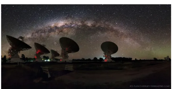
Figure 1.1: The Milky Way across the night sky as seen at the ATCA site. Image credit:

Alex Cherney (terrastro.com).

On the edge of the newly discovered “Laniakea” supercluster of galaxies (Tully

et. al. 2014) lies the Milky Way Galaxy (also known as the Galaxy), a barred spiral

galaxy host to 300 billion stars, including our own Sun, and the Solar system, which

is located in its outskirts at a distance of 27,000 light years ( ∼ 8kpc ) from the center

in the Orion-Cygnus Arm. The Milky Way gets its name from its appearance in the

night sky as a dim fuzzy glowing band stretching across the night sky, as seen in

Fig. 1.1. It is made up of a disk of stars which is 100,000 light years in diameter,

and only 1000 light years thick near the position of the Sun, decreasing away from

the center. The disk contains most of the Milky Way’s stars and all of its gas and

dust, with the total mass of 10

M

. The spiral arms are located in this disk and are

traced by the molecular clouds. These arms are thought to have formed because

of the density waves from the interaction between the stars and the gas in the disk

orbiting the Galaxy. As the molecular clouds are home to massive star formation,

1.1. The Milky Way 3 the star clusters near the spiral arms have relatively young massive stars. The H

regions, illuminated by the massive young stars also run across the spiral arms.

Periodic supernova explosions from the dying OB stars create expanding shells of material and fill the interstellar medium with hot ( ∼ 10

K ) X-ray emitting gas. The stars eventually disperse from their birth environment, and thus the disk contains a mix of young and old stars.

The disk of the Galaxy is surrounded by a spherical halo of stars. This halo is sparsely populated and contains stars worth total mass of ∼ 10

M

and virtually no gas and dust, and thus no star formation. Due to this, the halo stars are quite old and appear reddish in color. The small, spherical, densely packed globular clusters of about 10

− 10

stars contain about 1% of the halo stars. Some of the oldest stars in the Galaxy can be found in these 150 globular clusters. This halo of the stars and the Galaxy are embedded in the spherical dark matter halo extending for hundreds of kiloparsecs, which has a mass of ∼ 10

M

.

Figure 1.2: A sketch of out Galaxy showing different structural components, the disk, the bulge, and the halo. Image: Ka Chun Yu, Introduction to Astronomy.

Towards the center of the Galaxy is the flattened, elongated collection of stars

known as the Galactic Bulge. The bulge stars away from the center are older. They

have highly elliptical orbits, with largely random inclinations, although their aver-

age stellar motion is net rotation around the Galactic center. The center also con- tains a faint bar of the length of 1 − 5kpc . The nature of the bar is highly debated, with suggestions of a single bar, triaxial bulge, or two distinct nested bars. At the very center of the Galaxy lies a supermassive black hole (SMBH) Sagittarius A*

(Sgr A*) with a mass of 4 million solar masses, the protagonist of this thesis. The center of the Galaxy is shrouded in the intervening gas and dust. Thus it remains obscured in the visible light, and cannot be observed. But it appears bright in other wavelengths of the spectrum, which can pierce through the dust, and provide us with the landscape of the central region.

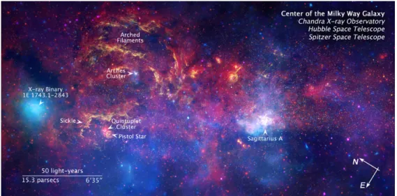
Figure 1.3: A combined image of the Galactic Center as seen from the Hubble Space Tele- scope in near-infrared, Spitzer Space Telescope in infrared, and Chandra X-ray Observatory in X-ray light. (Image credit: NASA/ESA/Spitzer/CXC/STScI).

The nucleus of the Milky Way is 100 pc across, which contains several stellar

clusters, such as the Arches Cluster and the Quintuplet Cluster, as well as fila-

ments of dust and gas which are heated up by the radiation from the stars, and are

birthplaces of young stars (yellow in color as seen fig. 1.3). The X-ray traces the

high energy emission from the accretion of material on compact sources and black

holes. Sagittarius A complex is the brightest region in X-ray light, arising from the

diffused gas that has been heated to several million degrees of temperature by stel-

lar winds, and outflows from stellar explosions and from the supermassive black

hole.

1.2. The Center of the Milky Way 5

1.2 T HE C ENTER OF THE M ILKY W AY

The inner few parsecs of the Milky Way galaxy is a complex and dynamic envi- ronment, with Sgr A*, the supermassive black hole at the dynamic center, and sur- rounded by the stellar cluster of young and evolved stars, interstellar medium with diffuse hot gas, molecular dusty ring and supernova-like remnants. It is a unique environment which allows for the study of the interplay of several phenomena, from star formation in the vicinity of the SMBH, physics of interstellar medium, to high energy emission processes associated with the accretion onto the black hole.

Being the closest available galactic nucleus environment, it can be studied with the resolution that isn’t possible to achieve with other galaxies. At a distance of ∼ 8 kpc, one arcsecond corresponds to 0.04 pc ( ∼ 1.2 × 10

cm). Thus the Galactic Cen- ter has been actively explored in radio, submillimeter, infrared, X-ray and _γ -ray wavelength with high angular and spectral resolution.

1.2.1 The Galactic Center Interstellar Medium

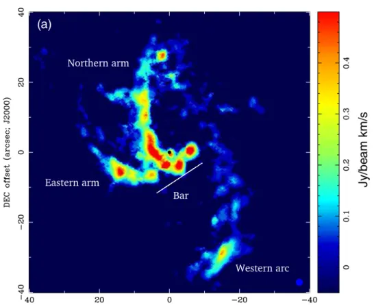
The interstellar medium in the GC region is mostly distributed in giant molecular clouds. The central few parsecs of the GC consist of a circumnuclear disk (CND) of neutral atomic gas, enclosing a cavity of relatively less density containing atomic and ionized gas. Close to Sgr A* within 1 − 1.5 pc lies a region called Sgr A West, which contains the mini-spiral. These are ionized clumpy filaments or streamers that orbit Sgr A*. 1.3 cm and 3.6 cm observations with Very Large Array (VLA) telescope have identified the features of the mini-spiral, viz. the Western arc, the Northern and Eastern arms, and an extended bar, as seen in fig. 1.4 (Ekers et al., 1983; Lo and Claussen, 1983; Serabyn and Lacy, 1985; Serabyn et al., 1988; Schwarz et al., 1989; Lacy et al., 1991; Herbst et al., 1993; Roberts and Goss, 1993; Liszt, 2003;

Paumard et al., 2004; Zhao et al., 2009). The Western arc of the streamer is most likely on a circular orbit, while the other components, i.e. the Northern, and Eastern arms and the bar penetrate deep into the central region within few arcsecond from Sgr A* and have highly elliptical orbits.

These filaments are ionized by the ultraviolet radiation from the massive young

stars. Of the 300 M

neutral atomic gas and few M

of warm dust, large fraction

is associated with the mini-spiral streamers, while the ionizing fronts may be inter-

faces between the low density and high density regions described by the neutral

ring (CND) (Paumard et al., 2004). In the central parsec, the average gas density is

lower than the surrounding CND. Study of the orbital motion of the streamers us-

Figure 1.4: Integrated 8.3 GHz image of the mini-spiral with marked components, the Western arc, the Northern and Eastern arms, and the extended bar. (Image: Zhao et al.

(2009)).

ing the VLA by Zhao et al. (2009) suggests that the CND and the enclosing streamers have their orbits at the same inclination relative to the plane of the sky. It is also suggested that these streamers are part of the inflow of gas due to dissipative loss of angular momentum from friction.

The circumnuclear disk is a dense torus-like ring or a disk surrounds the central parsec of the GC. It consists of clouds of dense molecular gas (Wright et al., 2001;

Herrnstein and Ho, 2002) and warm dust (Zylka et al., 1995) of about 10

solar mass

of gas and dust. It rotates around the center in a circular orbit, with a sharp edge at

1.5 pc and extends up to 5 − 7 pc from the center (Becklin et al., 1982; Guesten et al.,

1987; Christopher et al., 2005; Montero-Castaño et al., 2009). The Western arc of the

mini-spiral is thought to be the inner ionized surface of the CND. The studies of

1.2. The Center of the Milky Way 7

Figure 1.5: Schematic diagram of the Sgr A Complex as seen in the plane of the sky. (Image:

Herrnstein and Ho (2005)).

the velocity field and line emission, and the clumpiness of the CND suggest that the CND may be a transient structure, although there is no conclusive evidence for it (Guesten et al., 1987). Figure 1.5 shows the schematic of the larger scale structure of the interstellar medium in the Sgr A Complex, where the CND is surrounded by several thermal and non-thermal features, such as Sgr A East and the giant molec- ular clouds (GMCs).

1.2.2 The Star Clusters

The central parsec of the Galactic Center contains a dense star cluster, with Sgr A*

at the dynamical center. The observations of the GC stellar cluster at IR and radio

wavelengths over two decades have shown some intriguing characteristics. It is

an extremely dense cluster that contains mainly late-type red giants, including the asymptotic giant branch (AGB) stars. The spectroscopic observations also reveal hot early-type stars with strong winds exhibiting helium and hydrogen emission lines (“He stars”) (Krabbe et al., 1995; Genzel et al., 1996; Paumard et al., 2006; Tan- ner et al., 2006). These stars are generally characterized as the post main sequence Ofpe/WN9 stars, while some show characteristics of luminous blue variable (LBV) stars and Wolf-Rayet stars (Clénet et al., 2001; Eckart et al., 2004b; Moultaka et al., 2005).

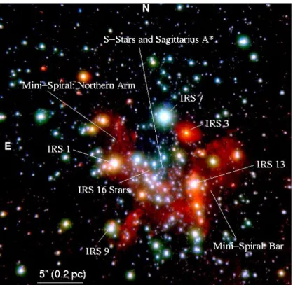
Figure 1.6: A composite NIR image ( λ = 1.5 − 4 µ m ) of the GC environment within the central parsec with the most prominent sources. The image is taken with NACO instrument at European Southern Observatory’s Very Large Telescope. Image: GC webpage of I.

Physikalisches Institut, University of Cologne.

The presence of such young stars in the immediate vicinity of the SMBH is

not completely understood. These stars are too young to have formed away from

the center and migrated inwards while it is thought that the extreme tidal forces

due to the presence of the supermassive black hole, the strong magnetic fields and

stellar wind may make star formation impossible in the region. But recent study

1.2. The Center of the Milky Way 9 of hydrodynamical simulations of the IRS stellar cluster 13 complex by Jalali et al.

(2014) has shown that orbital compression of the clumps orbiting the SMBH on the elliptical orbit can not only not hinder but even assist the star formation by increasing the gas densities in the clump to critical limit and overcoming the tidal density of the black hole. Potentially younger objects have been discovered in the central parsec of Sgr A* that hint towards very recent or ongoing star formation (Eckart et al., 2003, 2004b, 2005; Moultaka et al., 2004a,b; Muži´c et al., 2008). The GC also contains several luminous extended sources, which have now been known as bow shock sources, such as IRS 1W, 2, 5, 10W, and 21. These are caused by bright stars expelling strong winds through the ambient gas and dust of the northern arm (Tanner et al., 2002, 2003, 2005; Rigaut et al., 2003; Eckart et al., 2004b; Geballe et al., 2004). Some of these stellar sources will be discussed later in detail in chapter 4.

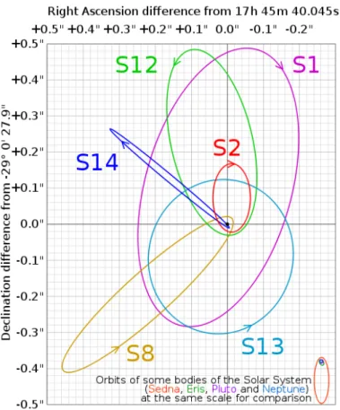
Figure 1.7: Inferred orbits of S-cluster objects around the supermassive black hole Sgr A*

obtained from the data from Eisenhauer et al. (2005).

The central arcsecond near to Sgr A* has a star cluster containing high velocity stars called the S-star Cluster. The NIR observations from 8 − 10 m class telescopes equipped with adaptive optics have enabled to identify and study closely the stars in the extreme vicinity of the SMBH. These S-stars orbit around Sgr A* at extremely high velocities in highly eccentric and inclined orbits. The precise measurements of the positions and proper motions of these stars has allowed for the determination of trajectories of 20 stars, which has been used for the calculation of the mass of the SMBH as well as relativistic effects on the central stellar cluster due the the black hole (Genzel et al., 1997; Schödel et al., 2002; Ghez et al., 2003; Gillessen et al., 2009a,b). Of these S-stars, S2 is the brightest star with the shortest orbital period of ∼ 15.9 years. Its motion was tracked for its full orbital period and was used to confirm the presence of the supermassive black hole and precisely determine its exact mass (Schödel et al., 2002; Ghez et al., 2003).

In 2012, a faint, dusty object was discovered in the S-star cluster, approaching Sgr A*, which is now called DSO/G2 (Gillessen et al., 2012, 2013; Eckart et al., 2013).

From the first observations, the object was thought to be made up of pure dust and gas, with a mass 3 times the mass of the Earth. Further observations and analysis pointed towards presence of stellar source at the center that is surrounded by a cloud of gas and dust. It was supposed to undergo its closest approach passage to the SMBH during Spring of 2014 at a distance of 200 AU. The discovery raised several questions. Would the object be destroyed by the tidal forces of the SMBH or would it survive the closest approach? How much of its mass would get accreted on to the black hole, and will it be enough to cause large variations in the flux density to brighten up Sgr A* across all wavelengths? This sparked a frenzy of observations from multiple telescopes (including observations I performed in 2013

& 2014, see section 2.3.2 for details). In section 3.6.1, I will discuss in details the results of the observations and conclusions of the DSO flyby.

1.2.3 Sagittarius A*

In 1971, Lynden-Bell and Rees (1971), by applying the then speculative black hole

model for quasars to the Milky Way, pointed out that the Galaxy should contain

a supermassive black hole at its center, which might be detectable with radio in-

terferometry. A compact radio source was subsequently observed by Balick and

Brown (1974) using the Green Bank Telescope of the National Radio Astronomy

Observatory (NRAO). It was then later confirmed by Westerbork and Very Large

Baseline Interferometry (VLBI) observations (Ekers et al., 1975; Lo et al., 1975), and

1.2. The Center of the Milky Way 11 was named as Sagittarius A*. It was discovered that Sgr A* was located near the dynamical center of the streamers in the nucleus from the high resolution VLA ob- servation Brown et al. (1981).

Sgr A* is one of the brightest radio source in the sky. It is always visible in this wavelength regime as its intensity never falls below the detection limit. Thus it can be monitored continuously in the radio regime. In contrast, Sgr A* is not detectable in IR and X-ray regime in its quiescent state and becomes visible only in its flaring state. Thus radio interferometric observations, thanks to the radio brightness of Sgr A*, allow us to study the SMBH at very high resolution.

One of the important question — how well does Sgr A* actually coincide with the dynamical center of the stellar cluster — was answered by radio observations.

The detection of SiO masers in the IR stars in both NIR and millimeter wavelengths within central arcsecond of Sgr A* led to the precise calculation of NIR reference frame, and the location of Sgr A* to within 30 mas in the NIR frame (See chapter 4 for details). The radio interferometric observations of the GC by Reid et al. (1999, 2003) with the Very Long Baseline Array (VLBA) have provided an accurate mea- sure of the position and proper motion of Sgr A* with respect to the extragalactic sources. From these observations they estimate that Sgr A* has a peculiar motion of −18 ± 7 kms

towards positive galactic longitude and −0.4 ± 0.9 kms

towards the north Galactic Pole (Reid and Brunthaler, 2004). No significant acceleration was detected in the motion of Sgr A*. These values are consistent with the zero proper motion. The simulations of the stellar motions of the central star cluster and the proper motion of Sgr A*, the estimated lower limit on the mass of Sgr A* is 0.4 × 10

M

within few AU. This result, along with the IR observations of the proper motions of S-cluster stars around Sgr A* has led to the conclusion that the radio source Sgr A* is associated with a supermassive black hole with a mass of 4 × 10

M

, which is at the dynamical center of the central stellar cluster.

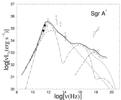
Thanks to multiwavelength observations of the GC, the spectrum of Sgr A* is

well-known. Sgr A* is known to be extremely dim compared to other objects in the

same class, radiating at roughly nine orders of magnitude lower than the Edding-

ton limit, which is the theoretical maximum limit at which black holes can accrete

given mass. The low luminosity of Sgr A* can be partly explained by the accretion

rate, which is significantly lower than the possible Eddington accretion rate. Fig. 1.9

shows the spectral energy distribution (SED) of Sgr A* in its quiescent phase across

Figure 1.8: The figure shows apparent motion of Sgr A* on the plane of the sky. Position residuals of Sgr A* relative to extragalactic source J 1745 − 283 is plotted along with 1 − σ error bars. The dashed line represents the variance-weighted best-fit proper motion, and the solid line gives the orientation of the Galactic plane. Image: Reid and Brunthaler (2004).

radio, near-infrared and X-ray wavelengths. The low frequency spectrum at cen-

timeter wavelength rises slowly with spectral index of α = 0.1 − 0.3 (the spectral

index _α is given as S

∝ ν

). The spectral index increases to _α = 0.5 at higher fre-

quencies, and peaking at α = 0.7 at 2 − 3 mm. This is known as the ‘submillimeter

bump’. This excess is probably due to the synchrotron self-absorption radiation

from the innermost optically thick region of the accretion disk. The turnover at

the submillimeter wavelengths happens as a result of the transition from optically

thick to optically thin, and the inner accretion region becomes transparent to the

synchrotron radiation. The spectral index of this part of the spectrum is negative

1.2. The Center of the Milky Way 13

Figure 1.9: Spectrum of Sgr A*. Image: Yuan et al. (2003b).

( α < 0 ), though the measurement of the index value of the quiescent spectrum at infrared & X-ray wavelength is not possible as the value varies with flux.

The models for the SED of Sgr A* have to explain the discrepancy between the Eddington luminosity and the observed luminosity. The most successful model to explain the low luminosity was the advection dominated accretion flow model (ADAF) which assumes a radiatively inefficient accretion flow. It involves an opti- cally thin, but geometrically thick accretion disk. Since the accretion disk is thick, the radial velocity and temperature are much larger and density of accretion flow is lower. Estimates from the observations of radio and submillimeter polarization (Bower et al. 2003; Marrone et al. 2006) predict significantly lower electron densities in the accretion region of Sgr A*, implying that most of the material does not reach the central black hole. This leads to the radiative time scales to be longer than the accretion time scale. Thus the accretion flow energy is not radiated away, but stored as thermal energy, thus leading to observed low efficiency.

1.2.4 Flaring of Sgr A*

Observations of the flux density of Sgr A* over different wavelength regimes have

shown that it is a highly variable source in all wavelengths, from NIR & X-ray to

radio and submm (Baganoff et al., 2001; Genzel et al., 2003; Eckart et al., 2006b, 2008, 2012; Yusef-Zadeh et al., 2006a,b; Li et al., 2009; Dodds-Eden et al., 2009; Kunneriath et al., 2010). This variability has been observed over wide range of time periods, from few minutes to few hours to few days. The first simultaneous multiwave- length observations were carried out by Eckart et al. (2004a). Since then, several such observations have been carried out, in which variations in the flux density of Sgr A* (called flares) were detected in NIR, X-ray, as well as in radio and submm regime. The radio/submm flares have been demonstrated to follow the brightest simultaneous NIR/X-ray flares with a delay of ∼ 100 min, indicating a link between flaring activity in different regions (Eckart et al. 2004a, 2006b, 2008; Marrone et al.

2008; Yusef-Zadeh et al. 2006b, 2008).

Several models have been proposed to explain the flaring activity of Sgr A*

with varying merits. Some of the prominent models are the adiabatically expand- ing plasmon model, the Jet-model with a weak jet, and the rotating hotspot model.

The study of the variability of Sgr A* can be helpful in understanding the physical processes in the vicinity of the SMBH, and understand the basic emission mecha- nisms of the accretion disk. The flaring activity of Sgr A* at mm wavelength will be discussed in detail in chapter 3.

1.3 O UTLINE

In this thesis, I will present the radio interferometric observations of the GC with Australia Telescope Compact Array (ATCA) at 3mm, which were carried out be- tween 2010 − 2014 . In chapter 2, I will introduce the basics of radio interferometry, as well as provide the details of observations and data reduction. This thesis con- sists of two main parts:

• The flaring activity of Sgr A* In this part (Chapter 3) I will discuss the results

of the monitoring of flaring activity of Sgr A* at 3mm wavelength. I will

present the methods used to obtain flux and light curves, and calculating the

variability of Sgr A*. I will present the results of the modeling of the observed

flares with the expanding plasmon model, and the analysis of the individual

flares. I will also discuss various models that have been used to study the

flaring of Sgr A*.

1.3. Outline 15

• SiO maser sources in the central parsec In Chapter 4, I will present the SiO maser sources that were detected within the central parsec of the Galactic Center during the 3mm observations with ATCA. I will describe the tech- nique used to detect the maser sources, and the method to compute the pre- cise positions and proper motions of the detected sources. I will then discuss the results and properties of the SiO masers.

In Chapter 5, I will present the summary and conclusions of the thesis.

C

2

R ^ADIO I NTERFEROMETRY , O BSERVATIONS , ^AND D ^ATA R ^EDUCTION

“There is a theory which states that if ever anyone discovers exactly what the Universe is for and why it is here, it will instantly disappear and be replaced by something even more bizarre and inexplicable.

There is another theory which states that this has already happened.”

— Douglas Adams, The Restaurant at the End of the Universe

2.1 R ADIO A STRONOMY

For most of the human existence, the view of the Universe was restricted to the vis- ible light. With the advances in electromagnetic theory in the 19th century, it was understood that objects could emit radiation apart from optical light. Radio waves were first postulated from the electromagnetic equations of James Clerk Maxwell and were subsequently discovered by Heinrich Hertz in 1887. The first practical ra- dio transmitters and receivers were developed by Guglielmo Marconi in mid-1890s.

The first astronomical discovery of radio source was done by Karl Jansky in 1933 when his antenna serendipitously discovered the radiation from Milky Way, and is now considered as the birth of radio astronomy. The field of radio astronomy gained momentum when scientists and engineers, who had carried out research

17

on radar technology during the World War II, turned their attention to astronomy to develop observational and instrumentation techniques. It led to the discovery of 21-cm hydrogen line, the pulsars, the quasars, and the cosmic microwave back- ground radiation. And now radio astronomy has become one of the most important tools in astronomy and has been used complimentary to other wavelength astron- omy.

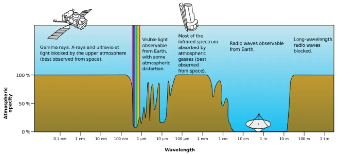
The Earth’s atmosphere is opaque to most of the electromagnetic spectrum, with two main windows, the optical-infrared band and the radio band, where it is transparent. This allows us to observe astronomical sources from the ground, as opposed to other wavelengths where satellite or balloon observations become necessary. The opacity of the atmosphere is shown in fig. 2.1. As seen from the figure the optical-NIR band is very narrow. Compared to that, radio wavelength can be useful between the wide window of wavelengths between 10 meters (30 GHz) to 0.3 millimeter (1 THz), which allows for the observations of wide range of astronomical sources, such as molecular gas, galaxies, active galactic nuclei etc.

The radio regime is divided into several bands: HF (below 30 MHz), VHF ( 30 − 300 MHz), UHF ( 300 − 1000 MHz), microwaves ( 1000 − 30000 MHz), millimeter-wave, and sub-millimeter-wave. At wavelengths smaller than 1 cm, only specific bands are available for observations as atmospheric absorption from vibrational transi- tion from atmospheric molecules such as CO

, O

, and H

O noise and attenuation creates limitations for observations. At wavelengths longer than 10 meters, the at- mosphere is completely opaque due to reflection from ionosphere.

The exceptionally broad frequency band of five orders of magnitude has two main consequences. The wide band allows for observations of a variety of astro- nomical sources, which arise from different thermal and non-thermal mechanism.

These include non-thermal radiation from galaxies, the strong radiation from the radio galaxies and quasars powered by SMBHs, thermal emission from cold inter- stellar gas, continuum emission from stars & pulsars, extrasolar planets and so on.

It also means different observation telescopes and techniques need to be developed to cover various bands of the radio spectrum.

2.1.1 Emission mechanisms

Electromagnetic theory describes two main types of emission processes: contin-

uum emission and line emission. The continuum emission process is further di-

vided into thermal and non-thermal emission. A continuum emission occurs when

2.1. Radio Astronomy 19

Figure 2.1: Electromagnetic transmittance of the atmosphere of the Earth over different parts of the electromagnetic spectrum. Image: NASA/jpl.nasa.gov

a source emits light in a continuous spectrum, as opposed to the line emission, which is quantized emission that gives rise to discrete lines or spectrum.

2.1.2 Thermal emission

Thermal radiation is the most basic form of radiation. All objects with a temper- ature emit continuous radiation that is proportional to the fourth power of their absolute temperature ( ∝ T

, Stefan-Boltzmann Law). There are two main types of thermal emission: the blackbody radiation, and the free-free emission.

Blackbody radiation:

A blackbody is an object that absorbs all the radiation incident on it and radiates a smooth spectrum of radiation. The peak of the radiation occurs at a frequency that is proportional to its temperature (see fig. 2.2) given by the Wien’s displacement law:

ν

= 5.879 × 10

T Hz

The power emitted per unit area per unit frequency is given by the Planck’s law:

B( ν , T ) = 2h ν

c

1

e

− 1 (2.1)

Figure 2.2: Blackbody radiation curves at different temperatures. Image: astron- omy.swin.edu.au.

where _ν is the frequency, k

is the Boltzmann constant, T is the absolute tempera- ture, and c is the speed of light. For radio wavelength region, the energy of photons is very low ( hν << k

T ), and thus the Rayleigh-Jeans limit is relevant over all of the radio window. The emitted power is then given by:

B(ν, T ) = 2h ν

k

T

c

(2.2)

The first examples of black bodies at radio wavelength were solar system plan- ets and asteroids. Stars, dust emission from interstellar medium, the cosmic mi- crowave background emission are some other examples of thermal blackbody ra- diation.

Bremsstrahlung:

Another form of thermal emission occurs from electrons traveling in ionized gas or plasma (HII region). It is produced by free electrons scattering off ions with- out being captured, hence called free-free emission or bremsstrahlung. In a plasma, the heavy immobile ions continuously cause slight deviations in the path of fast moving electrons. Since any charged particle that is accelerating also radiates, each deviation produces broad spectrum, and the power of the radiation emitted by the particle is given by the Larmour’s formula:

P = 2 3

q

v ˙

c

(2.3)

2.1. Radio Astronomy 21

Figure 2.3: Log-log plot of the blackbody curves for different temperatures. The straight line slope of the curve below THz ( 10

Hz) frequency shows that the Rayleigh-Jeans ap- proximation for the Planck law is valid for the radio frequencies. Image: web.njit.edu.

An inverse process to the free-free emission is the thermal bremsstrahlung absorp- tion, i.e., the absorption of energy from free-moving electron. An astronomical source radiating bremsstrahlung will show both the effects in its spectrum, the emission and absorption. Assuming a Maxwell-Boltzmann distribution of veloc- ities, the optical depth of the region is

τ

∝ Z

T

ν

n

d s (2.4) where n

is the electron number density. At low frequencies, τ

>> 1 , the HII region is optically thick, its spectrum approaches blackbody spectrum with temperature T, and its flux density varies as the square of the frequency. At high frequencies, the HII region is optically thin with τ

< 1 and its flux density changes as S

∝ ν

. 2.1.3 Non-thermal emission

If the characteristics of the emitted radiation are independent of the temperature of

the source, the radiation is known as non-thermal radiation.

Synchrotron emission:

Synchrotron radiation is a process that dominates much of high energy astro- physics. It is caused by the acceleration of charged particle moving at relativis- tic speeds in a magnetic field. It was first observed in early betatron experiments where the electrons were first accelerated to relativistic energies. In astronomy, only the radiation from an ensemble of electrons with a wide energy distribution is observed. Thus many of the details of the radiation are lost in the averaging pro- cess. In many cases, the synchrotron radiation is emitted by electrons which have power-law distribution:

N ( γ )d γ ∝ γ

d γ We can then express the emissivity as

²

∝ B

ν

where B is the magnetic field. For the electron energy spectrum with power law index p , the spectral index of the synchrotron radiation, defined by ²

∝ ν

, is α = (p −1)/2 . The spectral shape is thus determined by the shape of electron energy spectrum, rather than the shape of emission spectrum from individual electrons.

The radio emission from the Galaxy, supernova remnants, and extragalactic ra- dio sources is a result of synchrotron radiation.

Synchrotron self-absorption:

For every emission process, there is an absorption process. The process of scat- tering of emitted photons off of synchrotron electrons is known as synchrotron self- absorption. If the scattering process occurs many times, only the emission from the thin surface layer is observed, and the total flux observed is much smaller. For sufficient low frequencies and homogeneous source, the source becomes optically thick, and the flux density can be given by S

∼ ν

. At higher frequencies, the source is optically thin. The frequency at which the source changes from optically thick to optically thin is known as the turnover frequency, where the optical depth τ = 1 .

Inverse Compton scattering:

Inverse Compton scattering is the scattering of low energy photons to high en-

ergies by relativistic electrons so that the photons gain while the electrons lose the

2.1. Radio Astronomy 23

Figure 2.4: The spectrum of a homogeneous cylindrical synchrotron source for optically thick and thin region, with the turnover frequency _ν

. Image: ifa.hawaii.edu

energy. The inverse-Compton scattering is important for astronomy, especially ac- tive galactic nuclei and black holes, whose accretion disks produce a thermal spec- trum. The low energy photons produced in the accretion disk can be up-scattered to high energies by the high-Lorentz-factor electrons. In AGN and blazars, the syn- chrotron processes produce such low speed photons. These photons can then be up-scattered by the same electrons that produced them. This process is then called synchrotron self-Compton (SSC). Energy losses due to the inverse-Compton process are referred to as electron cooling.

The gamma ray bubbles arising from the center of the Milky Way observed with the Fermi-Gamma ray space telescope are thought to be due to the inverse Compton scattering of synchrotron radiation Su et al. (2010).

2.1.4 Line emission

Spectral lines are narrow emission or absorption features in the spectra of gases which appear at discrete frequencies. The spectral lines are a quantum phenomena.

The quantization of angular momentum gives rise to discrete energy levels in atoms

and molecules. The transitions between these discrete energy states in the physical

Figure 2.5: The illustration of the Gamma-ray bubbles arising from the GC. Image: Fermi telescope website.

systems result in spectral line emission and absorption. At radio wavelengths, the main sources of spectral line emission are the rotational transitions of molecules, such as CO, NH

etc. The 21-cm emission from the hydrogen line is the hyperfine transition between the two levels of the ground state of the electron in hydrogen atom.

Another type of emission that is important at the radio wavelengths is the natu- rally occurring stimulated emission in molecules, called as maser (microwave am- plification by stimulated emission of radiation). It is produced by the population inversion of the transition. The spectral lines are an important tool to study then physical and chemical properties of their sources. Hydroxyl (OH), water (H

O), and silicon oxide (SiO) masers are some of the most prominent sources of maser emission in millimeter astronomy. The SiO maser emission will be discussed in details in chapter 4.

2.2 R ADIO T ELESCOPES

Radio telescopes are the instruments used to detect the electromagnetic radiation

at radio wavelengths. Most modern radio telescopes are antennas with parabolic

2.2. Radio Telescopes 25

Figure 2.6: A simple sketch showing different components of a single dish radio telescope.

Image: http://www.haystack.edu/

reflecting dishes that can be pointed to the direction of the source of radiation. The parabolic dish reflects the radio waves to a subreflector located close to the prime focus, which then reflects the waves to the feed at the center of the reflector. The Ra- dio telescopes generally have a Cassegrain subreflector system. The signal from the feed is then sent to the receiver and amplifier system, which magnifies the faint radio signals. Throughout this process, the signal remains proportional to the strength of the incoming radiation, so that the resulting map is a true represen- tation of the emission from the source. The amplifiers are extremely sensitive and are normally cooled to very low temperatures to minimize interference due to the thermal noise. The spectral power received by the detector of unit projected area is called the source flux density S

, given by

S

= Z

sour ce

I

d _Ω (2.5)

here I

is the specific intensity or the spectral brightness of the source, in the units

of Wm

Hz

sr

, and d Ω is the solid angle between the observer and the source.

The flux density is measured in the units of Jansky (with 1 Jy = 10

Wm

Hz

). If we assume that the incident radiation is thermal in nature (even when it is actually not), we can express the specific intensity in terms of brightness temperature T

which is given by

T

( ν ) = I

c

2k

ν

= S

λ

2k

d Ω (2.6)

One of the important parameters of a telescope is its resolution. From the diffrac- tion theory, the resolution of a single dish radio telescope is given by

θ = 1.22λ/D (radian) = 2.52 × 10

λ/D (arcsec)

where D is the diameter of the dish. The resolution of single dish telescopes is lim- ited by the maximum size of the movable dish that can be constructed. The largest antenna also suffer from many issues such as tracking accuracy problem, gravita- tional distortion, solar heating etc. For example, a single dish telescope with aper- ture of 22 meters, operating at 3 mm wavelength will have a resolution of ∼ 35

. This is very low resolution compared to optical telescopes. Thus for high resolu- tion observations, single dish telescopes are not useful. To improve the resolution, single dish telescopes are combined to form an interferometer. Interferometry tech- niques combine several single antennas to synthesize a larger aperture, defined by the baseline B − the separation between the two antennas. Then the angular reso- lution is given as _θ = 1.22 λ /B . Thus, larger the separation between the individual antennas, better will be the resolution of the interferometer.

2.2.1 Interferometry and aperture synthesis

The basics of interferometry come from the Young’s double slit experiment, where coherent waves passing through two slits produce an interference pattern.

The van Cittert-Zernike theorem relates the spatial coherence function V (r

, r

) to the distribution of intensity of the incoming radiation I (s) received at two points r

and r

. It shows that the spatial correlation function V (r

,r

) depends only on r

− r

V

(r

, r

) = Z

I

(s)e

d Ω (2.7) Thus if one knows the mutual coherence function of the electric field, then the source brightness distribution can be measured by taking the Fourier transform.

Consider a two element interferometer, as shown in figure 2.7, with a separation

of b looking towards a point source in a direction s ˆ . Plane waves traveling from the

2.2. Radio Telescopes 27

Figure 2.7: A block diagram showing a simple two element interferometer. Image:

gmrt.ncra.tifr.res.in

distance source must travel extra distance of b sin θ to reach antenna 2, so the output at both the antennas is the same but the output at antenna 2 lags behind by the geometric delay of _τ

= b · s/c ˆ . If the output voltage at antenna 1 is V

= V cos(2 πν t ) then the output voltage at antenna 2 is V

= V cos(2 πν (t − τ

)) where t is time and ν is the radiation frequency. These signals are first multiplied at the correlator which gives

V

· V

= V

cos(2 πν t) cos[2 πν (t − τ

)] = µ V

2

¶

[cos(2 πν t − 2 πντ

) + cos(2 πντ

)]

and then takes a time average which removes the high energy term cos(2πν t − 2 πντ

) so that the final output is

R = 〈 V

V

〉 = µ V

2

¶

cos(2πντ

)

The correlator output R varies sinusoidally with the rotation of the Earth. This

sinusoidal pattern is called as the fringe pattern. The fringe phase depends on θ and

is a sensitive measure of the source position for projected baselines b cos θ longer

than several wavelength distances. Thus interferometers can measure the positions

of compact radio sources with great accuracy, with errors as small as ∼ 10

arcsec.

The response R of a two-element interferometer with directive antennas is the prod- uct of the power pattern of the individual antennas, and is known as the primary beam. The point-source response of an interferometer can be improved by adding more baselines. An interferometer with N antennas contains N (N − 1)/2 baselines.

Each of these can be connected together and the combined response is known as the synthesized beam.

The response of an interferometer to a spatially incoherent extended source with sky brightness distribution I

( ˆ s) can be obtained by assuming the extended source to be sum of independent point sources.

R(b) = Z Z

Ω

A(s)I

(s)e

d Ω d ν

Here A(s) is the effective collecting area of the antennas in the direction of s ˆ . The co- ordinates of the antennas when projected onto a plane perpendicular to the line of sight form a plane with axes u and v , thus called the ( u, v ) plane and they describe the projected separation and orientation of the elements. The coordinates l and m are direction cosines towards the astronomical source. Then the visibility function measured by the interferometer is given by

V

(u, v ) = Z Z

A

(l , m)I

(l , m)e

d l d m (2.8)

Taking the inverse Fourier transform of the above equation gives the source brightness distribution

I

(l, m) = A(l, m)I (l, m) = Z

−∞

V (u, v)e

d u d v (2.9)

Each observation of the source with a baseline and orientation forms a point in

the u − v plane, and a combined array of multiple baselines including the rotation

of the Earth fills up the plane, as can be seen from fig. 2.8. This can then be used to

construct the image of the source.

2.3. Observations 29

Figure 2.8: As an example of the u − v coverage of telescope array − the u − v coverage of Sgr A* with ATCA

2.3 O BSERVATIONS 2.3.1 The Telescope

We have used the Australia Telescope Compact Array (ATCA) for observing the

Galactic Center at 3 mm. ATCA is an array of six 22-m telescopes located at the

Paul Wild Observatory in Narrabri, New South Wales, about 550 km North-West

of Sydney, in Australia. It is operated by the Australia Telescope National Facility

(ATNF) of the Astronomy and Space Science division of the Commonwealth Scien-

tific and Industrial Research Organisation (CSIRO). The telescope operates in seven

observing bands: 20 cm, 13 cm, 6 cm, 1 cm, 7 mm, and 3 mm. The antenna 6 is per-

manently fixed in its location, which gives a maximum available baseline of 6 km,

but it is available for only select few array combinations. It is also not fitted with a

3 mm receiver, and thus is unavailable for 3 mm observations. Thus at 3 mm, the

angular resolution can range between 0.2

to 6

.

2.3.2 Observation details

We have observed the GC at 3 mm wavelength with the ATCA between 2010 and 2014. Out of these, the observations in 2013 and 2014 were performed by me. The location of ATCA has an advantage, as the GC passes almost overhead in the south- ern hemisphere, it allows us to observe the GC for more than 8 hours a day. The Compact Array Broadband Backend (CABB) of the telescope was upgraded in 2007.

This allows for observations with two 2048 MHz intermediate frequency (IF) bands.

The observations were performed with the spectral line mode at two different fre- quency bands at 86.243 and 85.640 GHz. These frequencies correspond to two ro- tational transition lines of the SiO maser (SiO J = 2 − 1 , v = 1 and J = 2 − 1 , v = 2 ).

The observations were conducted for approximately 10 − 12 hours per observation day. At the start of the observations, the bandpass calibrations were carried out for 30 min with PKS 1253 − 055 , and flux calibration with Uranus at the end of the observations. We observed Sgr A* with three sets of 25 min on-source observations which are in-between the observations of gain calibrators (see Table 2.1). For phase calibrations we used Sgr A* as it is strong enough source that it can be used as a self calibrator. The details of the observations are summarized in Table 1. The mapping and data reduction of the interferometer data was performed using the MIRIAD data reduction package.

The primary beam size of the telescope is ∼ 0.5 arcmin while the resultant sec- ondary beam size of the telescope is 1.95 × 2.28 arcsec . The antenna gain of ATCA strongly varies with the elevation angle. It is most efficient at the elevation angle of 60

and has a minimum value of efficiency at the elevation of 90

. The gravitational distortion of the dish causes small deformations in the shape of the dish. This de- formation is significant when observing sources closer to the horizon, and thus it limits the antenna efficiency at angles below 40

. Another factor to consider for the antenna gain is the angular separation between Sgr A* and the calibrator (Li et al.

2009). If we use a distant calibrator, the gain corrections resulting from it cannot fully compensate for the elevation effects. These effects show up in the light curve, and should be avoided. For this, the gain calibrators we used werenearby calibra- tors within 10

of Sgr A*, among them mainly PKS 1741 − 312 , as it is only 2.29

away from Sgr A*. Some secondary gain calibrators were also used for consistency.

As I have discussed in section 2.1, at millimeter wavelength, the atmosphere is

not transparent for electromagnetic waves. This can result in large fluctuations in

the gain. Especially for observations at lower elevation angles (less than 45

), we

observe strong variation due to the thick atmosphere. For certain compact array

2.3. Observations 31

Figure 2.9: The Australia Telescope Compact Array during observations in 2013.

configurations of the telescope, some antennas suffer from the shadowing effect, and it is significant for elevations of < 40

. Thus we only use the observational data above the elevation of 40

.

2.3.3 Data reduction

Once the observations are complete, the raw data obtained stored from the tele-

scope needs to be processed. Data reduction is a procedure for processing the raw

Table 2.1: The Log of observations of Sgr A* taken during 2010 to 2014. The dashes represent the days on which observations were not made. See section 3.4 for details.

Date Array Calibrators Start Time End Time

UT UT

2010

May 13

H214

1741−312 2010 May 13 11:04:45 2010 May 13 21:50:25 May 14 1622−297 2010 May 14 10:45:07 2010 May 14 22:07:40 May 15 1741−312 2010 May 15 10:10:30 2010 May 15 22:30:10

May 16 1622−297 2010 May 16 10:08:47 2010 May 16

2011

May 23

H214

1741−312 2011 May 23 09:57:43 2011 May 23 21:05:13 May 24 1741−312 2011 May 24 09:56:05 2011 May 24 21:24:17 May 25 1741−312 2011 May 25 10:01:13 2011 May 25 21:22:30 May 26 1741−312 2011 May 26 10:03:01 2011 May 26 21:17:33

2012

May 15

H214

1714−336 2012 May 15 08:23:47 2012 May 15 21:51:35 May 16 1714−336 2012 May 16 10:04:30 2012 May 16 21:45:22 May 17 1714−336 2012 May 17 09:49:17 2012 May 17 21:52:18 May 18 1714−336 2012 May 18 11:02:51 2012 May 18 21:56:46

2013

June 26 EW352 1741−312 2013 June 26 08:18:21 2013 June 26 20:44:37 June 27 EW 352 1741−312 2013 June 27− − − 2013 June 27− − − August 31 1.5A 1741−312 2013 August 31 03:36:08 2013 August 31 14:57:04 September 1 1.5A 1741−312 2010 September 2− − − 2013 September 2− − − September 14 H214 1741−312 2013 September 14 03:08:12 2013 September 14 13:27:58 September 16 H214 1741−312 2013 September 16− − − 2013 September 16− − −

2014

April 1 H168 1741−312 2014 April 1 14:54:24 2014 April 1 23:38:55 April 2 H168 1741−312 2014 April 2 13:37:58 2014 April 3 00:22:18 June 7 EW352 1714−336 2014 June 7 08:00:50 2014 June 7 19:00:02 September 26 H214 1714−336 2014 September 26 02:05:40 2014 September 26 12:44:31 September 27 H214 1714−336 2014 September 27 02:10:13 2014 September 27 12:40:51

data to correct for errors and interference in measurements. To perform the data re- duction, I used the MIRIAD data reduction software (Sault et al. (1995)). I start with flagging the data for bad data points as well as outliers and interferences. After that, several calibrations are performed. The aim of calibrations is to find out the relationship between the observed visibilities V

and the true visibilities V . For each baseline:

V

(t , ν ) = V (t, ν ) · G(t ) · B(t , ν )

here t is time and ν is frequency. G is the complex continuum gain, and B is the complex frequency-dependent gain (i.e., the bandpass).

• Bandpass calibration is a process of measuring and correcting the frequency-

dependent part of the gains B(t , ν ) . The antenna based complex gains vary

2.3. Observations 33 across the passband. These need to be corrected before the visibilities from individual frequency channels are averaged. Hence bandpass calibration is performed to estimate and correct for the bandpass shape.

• Amplitude calibration: The interferometers do not measure the absolute flux densities of the sources. Thus the relative flux density scale is usually set by observing an unresolved reference source whose flux density is believed to be stable and whose intensity has previously been measured on an absolute scale. In our case, planet Uranus was used as a flux calibrator.

• Gain calibration: Antenna based complex gains vary slowly with time with variation of the order of few tens of minutes. These slow variations are mea- sured and corrected using periodic observations of a secondary calibrator, which is not too far from the source.

• Phase calibration: The phase calibration determines the instrumental and at- mospheric phase effects by observing a point-like source that is not variable and whose position is well-known.

• Self calibration: The technique of self-calibration is used to make additional

corrections to the antenna gains as a function of time. This is similar to basic

calibration discussed above, the main difference being that self-calibration

procedure is often performed iteratively, each time with a better model, until

finally the sequence converges.

After performing these calibrations, a final image is produced using following steps:

The image produced by Fourier transform of the visibilities is called the dirty

image. Since the u − v plane is not sampled completely (as seen from fig. 2.8), it

causes imperfections in this image. The inverse Fourier transform of the sampling

function produces a point spread function, which is referred to as dirty beam in radio

astronomy. We assume that the dirty image is a convolution of the dirty image with

the dirty beam. The CLEAN algorithm attempts to deconvolve the dirty beam from

the dirty image, and convolves it with a Gaussian shaped clean beam to produce a

clean image.