Genome re-annotation and DNA motif identification in Brassicaceae species
Inaugural-Dissertation zur
Erlangung des Doktorgrades
der Mathematisch-Naturwissenschaftlichen Fakultät der Universität zu Köln
vorgelegt von
Vimal Rawat
II
Diese Arbeit wurde am Max-Planck-Institut für Züchtungsforschung in Köln in der Abteilung für Entwicklungsbiologie durchgeführt.
Berichterstatter:
Prof. Dr. George Coupland Prof. Dr. Thomas Wiehe
Prüfungsvorsitzender:
Prof. Dr. Martin Hülskamp
IV
New opinions are always suspected, and usually opposed, without any other reason but because
they are not already common .
— John Locke
(English Philosopher)VI
Table of Contents
List of Figures ... 4
List of Tables ... 5
List of Abbreviations ... 6
Summary ... 9
Zusammenfassung ... 11
Chapter 1 Introduction ... 13
1.1 Plant genome sequencing ... 15
1.2 Advancement in sequencing strategies ... 15
1.3 The impact of whole genome sequencing (WGS) ... 16
1.4 Genome re-sequencing and population-scale studies ... 17
1.5 Genome annotation: Coding and non-coding regions of a genome ... 18
1.5.1 Genome annotation: Coding regions of a genome ... 18
1.5.2 Genome annotation: Non-coding regions of a genome ... 21
Chapter 2 Improving annotation of Arabidopsis lyrata genome ... 29
Motivation and result summary ... 31
2.1 Introduction ... 33
2.2 Results and Discussion ... 34
2.2.1 Improving A. lyrata genome annotation using RNA-seq data ... 34
2.2.2 Validating differences in gene model structure ... 39
2.2.3 Comparison of version-2 annotation with other Brassicaceae ... 42
2.2.4 Enhanced usability of version-2 annotation: Alternate splicing events ... 45
2
2.4.4 Ortholog identification and InterProScan annotation ... 48
2.4.5 Identification of TE genes in version-2 ... 49
2.4.6 cDNA preparation and PCR ... 49
2.4.7 Differential gene expression and alternate splicing ... 49
Chapter 3 Uncovering an atlas of diurnal DNA motifs (DDMs) using Phylogenetic shadowing in Brassicaceae genomes ... 51
Motivation and result summary ... 53
3.1 Introduction ... 55
3.2 Results and Discussion ... 57
3.2.1 Time series transcriptomics data analysis for Arabidopsis and Arabis ... 57
3.2.2 Identification of diurnally expressed genes ... 57
3.2.3 Conservation of diurnal expression ... 59
3.2.4 Peak expression time (phase) based clustering of diurnal genes ... 60
3.2.5 Comparing expression profile of clock genes ... 63
3.2.6 Comparing expression profile of target genes of clock TFs ... 64
3.2.7 Leaf movement analysis ... 67
3.2.8 Functional analysis of diurnal genes ... 67
3.2.9 Defining regulatory region for DNA motif identification ... 73
3.2.10 Identification of CREs using Phylogenetic shadowing ... 75
3.2.11 Filtering non-significant diurnal DNA motifs (DDMs) and generating comparative motif set 79 3.2.12 Analysis of DNase I data for validation of tpsDDMs ... 80
3.2.13 Time point specific enrichment of DDMs in diurnal genes ... 81
3.2.14 Shifted enrichment profile of tpsDDMs ... 81
3.2.15 Identification and comparison of cis-regulatory modules (CRMs) ... 85
3.2.16 Loss and gain of diurnal expression ... 86
3.3 Materials and Methods ... 90
3.3.1 RNA-seq read mapping ... 90
3.3.2 Identification of diurnal genes ... 90
3.3.3 Leaf movement analysis ... 91
3.3.4 Defining regulatory regions for eight Brassicaceae genomes ... 92
3.3.5 Identification of conservation block and DNA motifs ... 92
3.3.6 Comparison of DNA motifs for both species ... 92
3.3.7 Motif co-occurrence analysis ... 93
3.3.8 Analysis of DNase I data ... 93
Chapter 4 Discussion ... 95
4.1 Annotating coding regions of genome ... 97
4.1.1 Improving the annotation of A. lyrata ... 97
4.2 Annotating non-coding regions of genome ... 98
4.3 Diurnal expression and its regulation ... 99
Appendix ... 103
Bibliography ... 107
Acknowledgement ... 127
Erklärung ... 129
Lebenslauf/ Curriculum vitae ... 131
4
List of Figures
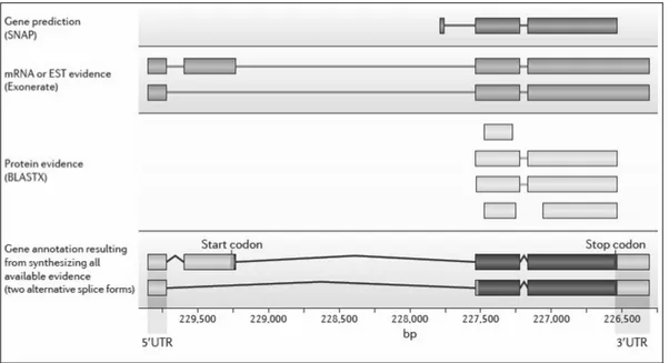
Figure 1 | Various layers in gene model annotation ... 20
Figure 2 | Examples of incorrectly annotated gene models ... 35
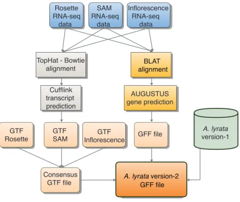
Figure 3 | Workflow for RNA-seq incorporation for version-2 annotation ... 37
Figure 4 | Overview of gene model annotation and gene length comparison ... 38
Figure 5 | Examples of wrong split and wrong merge cases in version-1 annotation ... 40
Figure 6 | Experimental validation of merged gene models in version-2 annotation ... 41
Figure 7 | Experimental validation of splitted gene models in version-2 annotation ... 41
Figure 8 | Comparison of identified orthologs in five Brassicaceae ... 43
Figure 9 | Comparison of gene features within five Brassicaceae ... 44
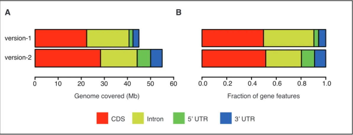
Figure 10 | Genic space comparison between version-1 and version-2 annotation ... 45
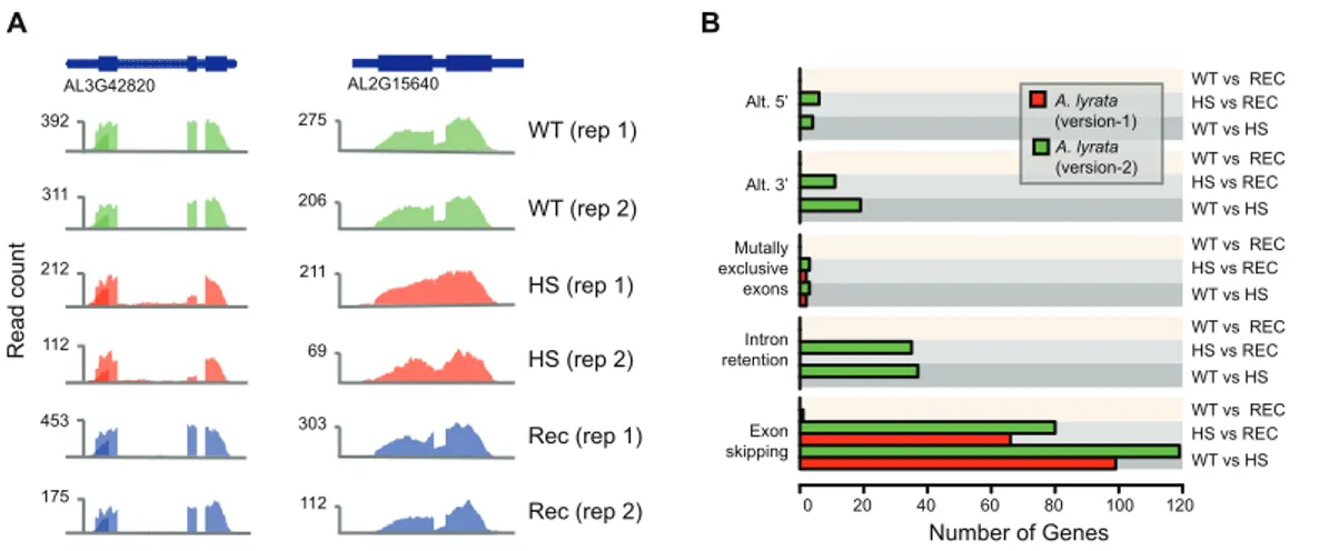
Figure 11 | Heat stress induced alternate splicing events ... 46
Figure 12 | Similarity analysis of samples collected at the same time over two days. ... 58
Figure 13 | Conservation of diurnal expression ... 60
Figure 14 | PCA of diurnal genes with imposed phase assignments... 61
Figure 15 | Bimodal distribution and phase difference of orthologs of diurnal genes ... 62
Figure 16 | Delayed expression of clock gene targets in Arabis compared to Arabidopsis ... 64
Figure 17 | Expression profile of clock genes in Arabidopsis and Arabis ... 65
Figure 18 | Circadian leaf movement data analysis ... 68
Figure 19 | GO term analysis in genes diurnal in both species. ... 72
Figure 20 | Defining regulatory regions for eight Brassicaceae ... 74
Figure 21 | Overview of Phylogenomic shadowing pipeline ... 77
Figure 22 | Atlas of diurnal DNA motifs ... 78
Figure 23 | Comparison of tpsDDMs ... 79
Figure 24 | Reduced cleavage frequency of DNase I around DDM instances ... 80
Figure 25 | Time point specific enrichment of DDMs ... 82
Figure 26 | Comparison of enrichment pattern for tpsDDMs in Arabidopsis and Arabis ... 84
Figure 27 | Comparison of intergenic lengths of diurnal genes ... 87
Figure 28 | DDM enrichment analysis for Arabidopsis ... 88
Figure 29 | DDM enrichment analysis for Arabis ... 89
List of Tables
Table 1 | Comparison of version-1 and varsion-2 annotation ... 38
Table 2 | Classification of all genes in six categories ... 58
Table 3 | Diurnal gene classification ... 59
Table 4 | Phase information of Arabidopsis clock genes and orthologs in Arabis ... 63
Table 5 | List of enriched functional categories in Arabidopsis diurnal genes ... 69
Table 6 | List of enriched functional categories in Arabis diurnal genes ... 69
Table 7 | List of enriched functional categories in diurnal genes with similar phase ... 70
Table 8 | List of enriched functional categories in diurnal genes with shifted phase ... 71
Table 9 | Orthologs for Arabidopsis and Arabis in six other Brassicaceae ... 75
Table 10 | Highest enrichment time point for DDM clusters (Arabidopsis and Arabis) ... 83
Table 11 | Significant pairs of co-occurring tpsDDM in different time point clusters ... 86
6
List of Abbreviations
ABA response element like ABREL
Average Avg.
Basic Local Alignment Search Tool BLAST
BLAST-like alignment tool BLAT
Base pair bp
Biological rhythms analysis software system BRASS
CCA1 binding site CBS
Cross Correlation CC
Circadian clock associated 1 CCA1
Complementary DNA cDNA
Coding sequence CDS
Chromatin immunoprecipitation ChIP
Chromatin immunoprecipitation-sequencing ChIP- seq
Conserved non-coding sequence CNS
Cis-regulatory element CRE
Cis-regulatory module CRM
Circadian Time CT
Coefficient of variation CV
Diurnal DNA motif DDM
DNase I hyper-sensitive site DHS
Deoxyribonucleic acid DNA
Evening Element EE
Early flowering ELF
Expectation maximization EM
Expressed Sequence Tag EST
Fold change FC
False discovery rate FDR
Fragment Per Kilobase of transcript per Million mapped reads FPKM
genomic DNA gDNA
Gene Feature Format GFF
Gene ontology GO
High confidence HC
hidden Markov model HMM
Hours hrs.
Heat stressed HS
Hormone Up and Down box HUD box
Isoform sequencing Iso-seq
Kilobase kb
Low confidence LC
Late elongated hypocotyl LHY
Long terminal repeat LTR
Lux arrhythmo LUX
Markov cluster algorithm MCL
Morning element ME
Megabase Mb
micro RNA miRNA
Model-based Periodicity Screening MoPS
Massive parallel sequencing MPS
Next-generation sequencing NGS
Open reading frame ORF
Protein box PBX
Principal component analysis PCA
Polymerase chain reaction PCR
Phylogenetic Footprinting PF
Position-specific scoring matrix PSSM
8
Reverse transcription-PCR RT-PCR
Sequencing by synthesis SBS
Starch synthesis box SBX
Shoot apical meristem SAM
Single-molecule real-time SMRT
Sequencing by Oligo Ligation Detection SOLiD
Standard error in measurement SEM
Telebox TBX
Transposable element TE
Transcription factor TF
Transcription factor binding sites TFBS
Timing of CAB expression 1 TOC1
Time-point specific diurnal DNA motif tpsDDM
transfer RNA tRNA
Transcription start site TSS
Untranslated region UTR
Whole genome sequencing WGS
Wild-type WT
Summary
The DNA sequence analysis field has experienced a paradigm shift caused by the drastic reduction in the sequencing cost and time. With the availability of several reference genome assemblies, understanding of structural and functional aspects of genomes has started growing. Annotating a reference genome is the first and very crucial step that ensures its efficient usability to serve as a community resource. Unlike coding regions, non–coding regions do not translate into proteins but still play a central role in development and physiology of an organism by regulating gene expression. Identification and annotation of these regions are only initial steps, equally interesting and even more rewarding is to decipher the interplay between these two components of a genome.
Identification of cis-regulatory elements (CREs), the functional components of the non- coding genome, is paramount to our understanding regarding the gene expression regulation. The role of CREs in regulating rhythmic (diurnal) expression of thousands of genes has been reported in several plants species (including Arabidopsis thaliana) but still only a few CREs have been reported so far.
In the first project, using extensive RNA-sequencing data, I substantially improved the annotation and usability of a Brassicaceae species, Arabidopsis lyrata. Gene model coordinates for over 90% genes are corrected, with improved UTRs (untranslated regions) annotation. Over 2,000 genes are now annotated as transposable element (TE)-related genes and around 8% annotated with alternate transcripts. With hundreds of cases of gene-merge and gene-split, improved annotation also corrects coding space of the genome. Experimentally validated data for several such cases strongly supported updated annotation, highlighting the importance of employing species-specific RNA-sequencing data for genome annotation.
In the second project, I compared time-series transcriptomics data for two Brassicaceae
species, Arabidopsis thaliana and Arabis alpina. Around 30% genes were found under
10
assembled Brassicaceae genomes, I analyzed the conservation patterns in promoters of
orthologous diurnal genes. In total, I identified 54 and 45 DNA motifs for Arabidopsis
thaliana and Arabis alpina respectively. Over 65% motifs were found common for both
species including previously reported six motifs. Based on recently published open
chromatin data, around 30% of the DNA motifs revealed protected sites from an
endonuclease (DNase I), indicating their potential role as protein-binding sites. Several
phase-specific co-occurring DNA motifs pairs were found conserved in both species,
including previously known Evening Element (EE) and ABA Response Element Like
(ABREL) pair, underlining the broad conservation of cis-regulation of diurnal expression.
Zusammenfassung
Das Feld der DNA-Sequenzanalyse hat sich, vor allem durch die drastisch gesunkenen Sequenzierungskosten sowie durch den verminderten Zeitbedarf, stark gewandelt. Mit der Verfügbarkeit mehrerer Referenzgenomassemblierungen hat ein wachsendes Verständnis der strukturellen und funktionellen Aspekte des Genoms begonnen. Die Annotation eines Referenzgenoms ist dem entsprechend ein erster wichtiger Schritt, der einer effizienten Nutzung als gemeinschaftlicher Ressource dient. Im Gegensatz zum codierenden Teil des Genoms wird der nicht-codierende Teil nicht in Proteine übersetzt, spielt aber dennoch eine zentrale Rolle in der Regulierung der Genexpression und damit in der Entwicklung und Physiologie von Organismen. Mit der Identifizierung und Annotation dieser Teile des Genoms ist jedoch nur ein erster Schritt getan. Darüber hinaus ist die Entschlüsselung des Zusammenspiels von codierenden und nicht-codierenden Bereichen eine ebenso interessante wie aufschlussreichere Fragestellung. Die Identifizierung von Cis- Regulatorischen Elementen (CREs) sowie deren Funktion in der Genregulation und Expression ist entscheidend für das Verständnis des nicht-codierenden Teils des Genoms.
Für die tagesrhythmische Expression tausender von Genen in verschiedenen Pflanzenarten (einschließlich Arabidopsis thaliana) spielen die CREs eine zentrale Rolle, dennoch sind bis heute nur wenige CREs beschrieben.
Im ersten Teil meiner Arbeit wurde durch die Einbeziehung von umfangreichen RNA-
Sequenzdaten, ist es mir gelungen die Annotation und deren Benutzerfreundlichkeit für
eine Brassicaceae Art, Arabidopsis lyrata, wesentlich zu verbessern. Für mehr als 90 %
der Gene haben sich Genmodellkoordinaten aufgrund der verbesserten „Un-Translated
Region“-basierten Annotation verändert. Tausende Gene sind dadurch als „Transposable
Element“ annotiert worden, zudem ist für rund 8 % der Gene alternative Transkription
identifiziert worden. Hunderte Gene wurden entweder mit anderen Genen zu einem Gen
verbunden oder voneinander getrennt, so konnte die Annotation des codierten Teils
12
Zwischen den Arten wurde eine interessante Verschiebung der Phase von rhythmisch zirkulierenden Genen beobachtet. Eine ontologische Analyse bezüglich des vermehrten Auftretens von tagesrhythmisch exprimierten Genen zeigt, dass Kohlenhydratstoffwechsel-assoziierte Gene am stärksten in ihrer Phase verschoben, Lichtsignal-assoziierte Gene hingegen am wenigsten beeinflusst sind. Darauf aufbauend wurden mittels „Phylogenetic Shadowing“ CREs gesucht die vermehrt in der tagesrhythmischen Genregulation vorkommen. Dabei war es möglich die Konservierungsmuster in orthologen Promotoren der tagesrhythmischen Gene anhand von mehreren kürzlich assemblierten Brassicaceae Genomen zu analysieren. So wurden 54 beziehungsweise 45 DNA-Motive für Arabidopsis thaliana und Arabis alpina gefunden, wobei die beiden Arten mit über 65 % übereinstimmten - inklusive sechs bekannter Motive. Basierend auf öffentlich zugängliche „Open Chromatin“ Daten wurde festgestellt, dass circa 30 % der DNA-Motive einen Schutz vor Endonuklease (DNase I) zeigen, was eine mögliche Rolle als Proteinbindungsstellen nahelegt. Mehrere zusammen auftretende und phasenspezifische DNA-Motiv-Paare wurden in beiden Arten gefunden, darunter bereits bekannte wie das „Evening Element“ und „ABA-Response-Element“
Paar, denen konservierte tagesrhythmische cis-regulierte Expression zugrunde liegt
Chapter 1
Introduction
14
1.1 Plant genome sequencing
The release of reference genome of Arabidopsis was a major milestone in plant biology (The Arabidopsis Genome Initiative, 2000) Being the first plant genome and the third multicellular genome to be sequenced after nematode Caenorhabditis elegans (The C.
elegans Sequencing Consortium, 1998) and insect Drosophila melanogaster (Adams et al., 2000), it had a huge contribution towards beginning of plant genomics era. In Arabidopsis, functional and evolutionary studies became possible with the availability of high-quality reference genome (Koornneef & Meinke, 2010).
The recent introduction of high-throughput sequencing technologies dramatically reduced the difficulty, time, and cost associated with it. With these advancements in sequencing, plant community has witnessed a sharp rise in the successfully completed several plant genome projects, including fairly large and economically important plants such as rice ((Goff et al., 2002); (Yu et al., 2002.); (International Rice Genome, 2005), soybean (Schmutz et al., 2010), maize (Schnable et al., 2009), chickpea (Varshney et al., 2013) and wheat (Wheat Genome Sequencing Initiative, 2014).
1.2 Advancement in sequencing strategies
Sequencing for the Arabidopsis reference sequence was performed using (semi-
automated) dideoxy Sanger sequencing ((Sanger et al., 1977); (Hunkapiller et al.,
1991)). This method is extremely time consuming and expensive. In 2005, a new
sequencing technology, sequencing by synthesis (SBS) developed by 454 Life Sciences
made sequencing cheaper and quicker ((Ruparel et al., 2005); (Margulies et al., 2005)). In
this method, DNA sequences are determined by synthesis or addition of nucleotides to the
complementary DNA strand rather than chain-termination (as in dideoxy Sanger
sequencing method). In 2006, Solexa Inc. (acquired by Illumina in early 2007) released
Genome Analyzer® that was also based on SBS technology (Margulies et al., 2005). In
16
sequencing (MPS) system of next-generation sequencing (NGS) technology.
Simultaneous sequencing of spatially separated DNA templates in a massively parallel fashion facilitated quick sequencing (Shendure & Ji, 2008).
Sanger sequencing (1
stgeneration method) and SBS (2
ndgeneration method) both required prior in vivo amplification (molecular cloning) or in vitro (by polymerase chain reaction (PCR)), while 3
rdgeneration sequencing methods (PacBio RS sequencer launched by Pacific Biosciences) have no such requirement of prior amplification as sequencing of single molecules is performed ((Eid et al., 2009); (Rothberg et al., 2011)).
Apart from the amplification free approach, another striking feature of the 3
rdgeneration sequencing methods was sequencing of longer reads (up to dozens of kilobases (kbs)) compared to 2
ndgeneration sequencing platforms (up to 700 base pairs (bps)).
1.3 The impact of whole genome sequencing (WGS)
The decision of selecting a species for sequencing is taken after considering several criteria such as scientific or economic importance, the size of the research community, genome size, ploidy level, availability of genetic and physical maps, etc. A substantial fraction of sequenced plant genomes belong to crop species and have been sequenced for particular research purposes by large and active research communities ((Wheat Genome Sequencing Initiative, 2014); (Schnable et al., 2009); (Mayer et al., 2012); (Velasco et al., 2010); (Shulaev et al., 2011); (Slotte et al., 2013); (Willing et al., 2015)). For last few years, this trend is being challenged and projects like Genome10K (https://genome10k.soe.ucsc.edu/) launched with the objective of sequencing a genomic zoo, a collection of DNA sequences representing the genomes of 10,000 vertebrate species, roughly one from every vertebrate genus (Genome 10K Community of Scientists, 2009).
As more and more genomes are getting sequenced, novel biological aspects are getting elucidated, such as questions on adaptation or evolution ((Dassanayake et al., 2011);
(Slotte et al., 2013); (Willing et al., 2015)). With addition of each new genome, our
understanding of genome biology increases and sometimes, the previous hypotheses are
refined or re-defined. For example, the genome of banana (Musa acuminata) and tomato
(Solanum lycopersicum) enhanced understanding of not only whole-genome duplications but also, its role in shaping the evolution of monocot and dicot plants ((D’Hont et al., 2012); (Sato et al., 2012)).
1.4 Genome re-sequencing and population-scale studies
Once the genome sequence for a species is available, it becomes possible to catalog sequence variations with associated biological consequences. This includes naturally occurring sequence variations and mutations introduced by random mutagenesis ((Page &
Grossniklaus, 2002); (Østergaard & Yanofsky, 2004); (Schneeberger & Weigel, 2011)).
Identification of these sequence differences is crucial to connect genotype to phenotype.
Though, sequencing a genome has become quicker, inexpensive and less complicated, assembling a genome is still a challenging task ((Schatz et al., 2010); (Earl et al., 2011);
(Salzberg et al., 2012)). Therefore, sequencing individual genomes and mapping sequencing data to get an estimate of sequence variation became popular (known as re- sequencing). Re-sequencing not only simplified sequence variation detection but also, made sequencing with lower depth possible. This is essential to accommodate multiple genomes within the same cost. This approach is either applied to whole genome context (whole genome re-sequencing) ((Ossowski et al., 2008); (Huang et al., 2009)) or to specific loci of interest (targeted enrichment re-sequencing) ((Gnirke et al., 2009);
(Mamanova et al., 2010)).
Re-sequencing involves mapping of randomly fragmented millions of DNA pieces
(typically around 100 bp long) back to reference sequence with high accuracy. When
dealing with small pieces of DNA, distinguishing sequencing/assembly errors from real
sequence variations is a non-trivial task. While alignment tools such as Basic Local
Alignment Search Tool (BLAST) (Altschul et al., 1990), BLAST like Alignment tool
(BLAT) (Kent, 2002) are fast and powerful but not specialized for mapping enormous
18
2009) along with work by (Gan et al., 2011)) is worth mentioning in this context. In the year 2009, Schneeberger et al. demonstrated that simultaneous alignment of short read data against several genomes not only provide access to highly diverged regions that are difficult to map otherwise, but also limits alignment errors near Indels. In the same year, Gan et al. highlighted the importance of analyzing genomic data along with transcriptomics data to interpret functional consequences associated with sequence variation in “reference-free” manner. Recent advancements in alignment methods resulted in developing a reference-sequence-free approach to benefit non-model species ((Nordström et al., 2013); (Ratan et al., 2010); (Iqbal et al., 2012)). The possibility to re- sequencing genomes led to ambitious projects like the 1001 Arabidopsis genome project focusing on the population dynamics by sequencing hundreds of individual genomes ((Weigel & Mott, 2009); (Cao et al., 2011); ).
1.5 Genome annotation: Coding and non-coding regions of a genome 1.5.1 Genome annotation: Coding regions of a genome
Once a high-quality genome sequence is available, next step is to annotate the gene models (referred to as coding region of the genome). Genome annotation broadly divided into two distinct phases. The first phase includes structural annotation of genome that involves, precise identification of sequence elements such as introns, exons, start codon, stop codon, etc. The second phase is functional annotation where the aim is to assign biological function to genomic elements.
Identification and masking repeat sequences are the initial steps of the genome annotation. Repeat masking is important to inform gene prediction tools to exclude these regions from gene prediction. Tools used for repeat identification either involves homology-based searches such as LTR_Finder (Xu & Wang, 2007), RepeatMasker (http://www.repeatmasker.org/webrepeatmaskerhelp.html), Censor (Kohany et al., 2006) etc. or de novo library-based search such as RepeatModeler (http://www.repeatmasker.org/RepeatModeler.html), RepeatScout (Price, et al., 2005) etc.
Frequently a combination of both approaches is used for repeat identification and
masking.
Ab initio gene tools (predictors) offer a fast and comprehensive solution for screening the genome for potential protein coding regions ((Norton & York, 2003); (Brent, 2005)).
Prediction is done for common features of a protein-coding gene such as start codon (ATG), stop codon (TAA, TGA, TAG), open reading frame (ORF), intron-exon boundaries and sometimes even polyadenylation sites (Salamov & Solovyev, 2000).
Present-day ab initio predictors are mostly based on hidden Markov models (HMMs) or more complex and improved versions of it (e.g. GHMM) ((Burge & Karlin, 1997);
(Lukashin & Borodovsky, 1998); (Korf, 2004); (Salamov & Solovyev, 2000); (Stanke &
Waack, 2003)). However, these tools have practical limitations in predicting UTRs and alternative isoforms. Moreover, despite using sophisticated models for gene prediction, ab initio methods suffer from a high false positive rate (Norton & York, 2003). Once transcriptional and protein sequence evidences became available, gene prediction tools were updated to utilize experimental data for further improvement in accuracy (Augustus (Stanke & Waack, 2003), SNAP (Korf, 2004), FGENESH (Salamov & Solovyev, 2000)).
Supplementing ab initio tool with (experimental) evidence data substantially improved its accuracy in filtering false positives. Traditionally, experimental data such as Expressed Sequence Tags (ESTs), cDNA or protein data are used to supplement prediction tool (Guigó et al., 2006). The newest addition to this list is RNA-sequencing (RNA-seq) data.
RNA-seq data is commonly used in two ways for gene prediction (Garber, 2011). First,
de novo assembly of RNA-seq reads, followed by transcripts mapping using long read
mapping tools such as Velvet (Zerbino & Birney, 2008). Alternately, RNA-seq reads can
be aligned to the genome sequence using split read aligners such as TopHat (Trapnell et
al., 2009), followed by transcripts reconstructing tools like Cufflinks. Figure 1
summarizes various evidences layers used to improve gene model (Robertson et al, 2010).
20
Figure 1 | Various layers in gene model annotation Source: (Yandell & Ence, 2012)
In second phase, genes can be functionally annotated by employing several approaches including sequence similarity searches, protein-protein interactions and functional assignment based on protein 3D folding or gene expression profiles. The most straightforward way to infer gene function is based on sequence similarity, using database-searching programs such as BLAST (Altschul et al., 1990) or PSI-BLAST (Altschul et al., 1997). Once a high scoring match is found in database, functional annotation is transferred to the query sequence. The success of this approach highly depends upon completeness and accuracy of information present in the database(s).
Several databases are available for functional annotation assignment: RefSeq NCBI database (Pruitt et al., 2012), UniProt/Swiss-Prot (Wu et al., 2006), Gene Ontology database (Ashburner et al., 2000), Pfam (Finn et al., 2006) etc.
Even for annotated genomes, additional data (e.g. additional RNA-seq data) can be used to improve existing genome annotations ((Li et al., 2011); (Eckalbar et al., 2013);
(Darwish, Shahan, Liu, Slovin, & Alkharouf, 2015); (Rawat et al., 2015)). Next challenge is to make such improved information available with version information. In a comprehensive review, Steven L Salzberg underlined the need of setting “guidelines” or
“community-wide accepted standards” for genome sequencing and annotation projects
(Salzberg, 2007). His emphasis was on setting a wiki for updating genome annotation
similar to what the Arabidopsis community successfully demonstrated through TAIR (https://www.arabidopsis.org/).
In chapter 2 of the thesis, I will present a study conducted to improve annotation of Arabidopsis lyrata, which was recently published in PLoS One (Rawat et al., 2015).
1.5.2 Genome annotation: Non-coding regions of a genome
Genome annotation efforts primarily focus on sequence with coding potential but a substantial fraction of the genome remains un-annotated. For instance, in gene dense Arabidopsis genome around 70% genome is not annotated (Lamesch et al., 2012).
However, information about the regulation of genes is encoded in this, so-called non- coding regions which is now has become an integral part of genome annotations.
Unlike coding regions, identification of non-coding regions is not straightforward due to high variation in location, size, and sequence composition. To identify functional non- coding elements, promoter regions of co-expressed genes can be compared ((Aerts et al., 2003); (Aerts et al., 2004); (Sarkar & Maitra, 2008); (Wrzodek et al., 2010); (Gao et al., 2013)). Another common approach to identify functional non-coding regions is to use evolutionary constraints through comparative sequence analysis. One prerequisite for this approach is the availability of multiple closely related genome sequences. Using comparative sequence analysis, several attempts have been made to uncover conserved non-coding sequences (CNS) in yeast (Kellis et al, 2003), insect ((Stark et al., 2007);
(Siepel et al., 2005)), worm ((Siepel et al., 2005)), vertebrates ((Siepel et al., 2005);
(Bejerano et al., 2004); (Boyle et al., 2008)) and plants ((Hupalo & Kern, 2013); (Lyons et al., 2008)).
Brassicaceae is an economically important family of flowering plants, including the
22
contributing to functional information, Brassicaceae seems ideal for non-coding region analysis. In the year 2013, Haudry and coworkers conducted a well-designed study with nine Brassicaceae genomes (six previously sequenced species and three new species) to identify 90,000 conserved non-coding sequences (CNSs). In this study, they could show that in Arabidopsis around 4% of the genome (4.5 Mb) is evolving under selection constraint and resides close to transcription start site (TSS) wih no coding potential identified (Haudry et al., 2013). One more interesting finding of this study was about similar CNS regions in Arabidopsis, despite nearly 40% smaller genome than Arabidopsis lyrata. (Hu et al., 2011). Besides, being the first large-scale attempt to discover and quantify CNS in Brassicaceae this study also highlighted the importance and abundance of non-coding elements.
1.5.2.1 Transcription regulation by cis elements
In plants, transcriptional regulation of gene expression is mainly controlled at gene promoters through cis-acting elements. ((Meshi & Iwabuchi, 1995); (Singh, 1998); (Liu et al., 1999); (Kaufmann et al., 2010)). Transcriptional regulation by transcription factors (TFs) binding in the promoter region of a gene, is a widely explored mechanism (Wray et al., 2003).
Arabidopsis has around 6-10% of its genes coding for transcription factors, which
underlines the importance and complexity of transcriptional regulation by TFs
((Riechmann et al., 2000); (Qu & Zhu, 2006)). Even if bound by the identical protein, TF
binding sites (TFBSs or cis-regulatory elements (CREs)) are not identical ((Palaniswamy
et al., 2006); (Priest et al., 2009)). To represent such complex sequence preference, all
TFBSs are used and referred to as DNA motif. In plants, CREs are short (generally
conserved) motifs of 5 - 20 nucleotides and usually found upstream of genes (Rombauts
et al., 2003). However CREs have also been found downstream of the TSS, for instance,
in the 1
stintron of the gene itself ((Zhang et al., 2012); (Sieburth & Meyerowitz,
1997); (Sheldon et al., 2002); (Kooiker et al., 2005)). A single promoter is typically
composed of many CREs allowing for different combinations of TFs to mediate different
expression responses of a gene.
1.5.2.2 Identification of cis-elements in promoter sequence
The main goal of the cis-regulatory analysis is to locate and annotate CREs. This knowledge then, can be transferred to a broader context for better understanding of gene regulation. Various experimental and computational methods have been employed for identification of cis-elements.
Classical DNA footprinting experiment was one of the first attempts to identify regions in promoter bound by regulatory proteins (Galas & Schmitz, 1978). An extension of this approach is DNaseI-sequencing ((Crawford et al., 2004); (Boyle et al., 2008)). This method is used to discover the regulatory regions by sequencing of regions sensitive to DNase I cleavage in genome-wide manner. Analysis of DNase I hypersensitive sites (DHS) has revealed novel binding sites and has proven extremely useful for discovery of CREs ((Crawford et al., 2004); (Boyle et al., 2008)).
A more specific method, chromatin immunoprecipitation (ChIP), involves crosslinking of DNA to a specific (already known) DNA-binding protein followed by isolation step using a specific antibody. The DNA bound to the protein can then be identified, using microarray chips (ChIP-Chip) (Ren et al., 2000) or by direct sequencing (ChIP-seq) (Johnson et al., 2007). Resolution-wise ChIP-seq outperforms ChIP-Chip, but the precise binding location of transcription factor remains difficult to determine using either method.
As an essential step, most of the studies with ChIP-seq experiment follow a
computational motif finding step to pinpoint the precise binding locations and sequence
preference. Although variability of most binding motifs and variable affinity make the
motif finding challenging (Park, 2009). Due to several such efforts, binding location and
sequence preferences of many Arabidopsis transcription factors are known including
TGA, Hy5, PIL5, SEP3, SVP, FLC, PRR5, PRR7 and CCA1 ((Fonseca et al., 2010); (Lee
et al., 2007); (Wu et al., 2012); (Kaufmann et al., 2009); (Gregis et al., 2013); (Deng et
al., 2011); (Nakamichi et al., 2012); (Liu et al., 2013); (Nagel et al., 2015)). Moreover,
recent efforts have been made to study changes in binding preferences of TFs when they
24
and sometimes lack properly defined controls (Park, 2009). Additionally, due to high complexity, it is sometimes difficult to implement these techniques in specific contexts.
Because of these limitations, computational approaches are a good alternative or supplement to CREs identification. Computational approaches are defined broadly into two groups; (i) identification of instances of known TFBS and (ii) de novo identification of unknown DNA motifs.
(i) The accuracy of identification largely depends on how (well) the motif is defined. One approach to define motifs with degenerated consensus sequences (using IUPAC representation) but this lacks information about the likelihood of observing alternate nucleotide on various sequence positions. Most common way to define a motif is a position weight matrix (PWM) or position- specific scoring matrix (PSSM) ((Stormo et al., 1982); (Stormo, 2000)). A PWM or PSSM is a 4 X N matrix (for DNA), where the four rows represent DNA bases (A, T, G, and C) and N is the length of TFBS. Elements of PWM reflect the likelihood of observing a particular nucleotide at that particular position, which is usually done after correction for a compositional bias of the background genome. Search for existing motif that is the identification of instances of the motif, seems fairly straightforward, but low complexity and degeneracy in the sequence of known motifs make searches prone to false positives. Recent developments in PWM matching approaches are majorly based on index-based algorithms. These approaches involve pre-processing of the target sequence(s) into index structure (mostly suffix tree) which then can be used for quick search of PWM match (Beckstette et al., 2006). Another approach is the online search approach where a simple sequential search is performed over the target sequence ((Liefooghe et al., 2009); (Salmela &
Tarhio, 2007); (Korhonen et al., 2009)).
TFs are frequently expressed in several different tissues (or cell types) and still manage to coordinate tissue-specificity via different interacting co-regulators.
Therefore, identification of single TF binding profiles, in isolation is not
sufficient for deciphering complex transcriptional networks. Likewise, CREs
are generally clustered into some relatively small stretches (a few hundred
bps), forming cis-regulatory module (CRM). Computational approaches to
identify relevant co-occurring TFBSs (potential CRM) have been developed to address this problem (Cister: (Frith et al., 2001.); ClusterBuster : (Frith et al., 2003) ; CisModule : (Zhou & Wong, 2004) ; ModuleSearcher : (Aerts et al., 2004); Clover: (Frith, 2004); ModuleDigger : (Sun et al., 2009);,COPS : (Ha et al., 2012)).
(ii) A frequently used approach for de novo discovery of (cis) regulatory elements is to find sequence elements with high occurrence in upstream regions of a set of genes regulated in the same way. Genes with similar functional annotation, co-expressed genes (in same species) or orthologous genes from closely related species are explored for de novo motif identification. Promoter sequence alignments of closely related species were quite successful in the discovery of regulatory elements, commonly known as phylogenetic footprinting ((Tagle et al., 1988);(Cliften et al., 2003)). Based on the same principle, phylogenetic shadowing ((Boffelli et al., 2003.), (Hong et al., 2003)) has later been developed to explore shorter (and more refined) regions of promoters of closely related species to reduce combinatorial complexity. Both approaches have limitations; co-expressed genes obtained from microarray or RNA-seq experiments represent steady-state mRNA levels and not necessarily provide co-regulated gene set. Moreover, wrong ortholog assignment, missing ortholog, ortholog diversification (species-specific duplication or evolution) and low (and in short stretches) conservation in promoters limit accuracy of these approaches.
There is a long list of tools available for de novo DNA motif identification (MEME: (Bailey & Elkan, 1994); AlignACE: (Roth et al., 1998); RSAT : (van Helden, André, & Collado-Vides, 1998); Weeder : (Pavesi, Mauri, &
Pesole, 2001); RSAT suite : (Thomas-Chollier et al., 2008); CisFinder :
26
Gibbs search; MEME and AlignACE belong to this group ((Bailey & Elkan, 1994); (Lawrence et al., 1993)).
In thesis chapter 3, I present a study to discover DNA motifs enriched in the promoter of diurnally expressed gene in Arabidopsis and Arabis alpina.
1.5.2.3 Importance of cis elements in diurnal expression
All organisms experience the daily change in light and temperature due to rotation of the earth. Synchronized gene expression in response to these cyclic environmental changes is referred to as diurnal gene expression. Plants sense the time of the day and prepare themselves even before the light become unavailable and temperature drops at night. For this, they need to synchronize expression of genes according to time of a day. This contributes to rhythmic gene expression, which is believed to be driven through an extensive network of diurnal and clock-regulated transcription factors (TFs) and their corresponding CREs ((Dunlap, 1999); (Harmer et al., 2000); (McClung, 2006); (Harmer et al., 2009); (Greenham & Mcclung, 2015)).
1.5.2.4 Cis elements enriched in genes under diurnal/circadian regulation
One of the earliest report connecting cis elements with rhythmic gene expression reported an AT-rich oligonucleotide, AAAATATCT, commonly known as Evening Element (EE) in promoters of evening-phased co-expressed cyclic genes (Harmer et al., 2000).
Subsequent experiments confirmed that its presence is enough to drive periodic evening- phased expression in genes. EE is bound by CCA1, a core component of the circadian clock. Later, several circadian clock-related (and diurnal) cis-regulatory elements have been discovered and described including another similar AT-rich element, CCA1 binding site (CBS), AAAAAATCT (Michael & McClung, 2002) HUD box (Hormone Up and Down box, G-box (CACGTG; (Giuliano et al., 1988)) etc. ((Hudson & Quail, 2003);
(Covington et al., 2008)). Knowledge about circadian or diurnal CRE was enormously
advanced with numerous time-course microarray-experiments, clustering of genes
according to the expression peak, and subsequent CRE identification using enrichment
analysis (Covington et al., 2008). Detailed analysis of phase-specific gene expression,
revealed CREs specific to different phases of a day; Morning Element
(AACCACGAAAAT) enriched in promoter of morning-phased genes, Telo-box
(AAACCC) and protein box (ATGGGCC) enriched in mid-night phased genes, and
GATA element was found to be enriched in afternoon and evening-phased genes
((Covington et al., 2008); (Covington et al., 2008)). Besides Arabidopsis, CREs are also
found in the cycling transcriptome of a monocot (rice) and a dicot (poplar) species. All
major classes of diurnal CREs, including morning (ME, GBOX), evening (EE, GATA)
and midnight (PBX/TBX/SBX) elements were found in both species (Filichkin et al.,
2011). This study provided evidence of conserved diurnal cis regulation between mono
and dicotyledonous species (Filichkin et al., 2011).
28
Chapter 2
Improving annotation of Arabidopsis lyrata genome
“Strive for continuous improvement, instead of perfection.”
Kim Collins (World champion sprinter, 2003)
30
Motivation and result summary
Arabidopsis lyrata is a close relative of Arabidopsis and frequently serves as an out-group in evolutionary studies. Additionally, it is also a model species for research on adaptation and molecular evolution. Even though its reference sequence is one of the few genome assemblies exclusively based on high-quality dideoxy sequencing data, its gene annotation was generated with limited RNA sequencing data. In the context of several on- going projects, we struggled with weaknesses of its current genome annotation.
Re-annotation of the genome using extensive RNA-seq data corrected the coordinates of around 90% gene models and introduced alternate isoforms for over 2,000 gene models.
This updated annotation includes hundreds of previously wrongly splitted and merged gene models, some of which were experimentally validated. Based on the RNA-seq data derived from a heat stress experiment, I also describe, how the new annotation enables an advanced analysis of differentially expressed isoforms in A. lyrata.
Contents of this chapter are published in PLoS One, 2015 with the title “Improving
annotation of Arabidopsis lyrata with RNA-seq data”.
32
2.1 Introduction
A. lyrata is a predominantly self-incompatible, perennial plant species from the Brassicaceae family that diverged from Arabidopsis approximately 10 million years ago (Hu et al., 2011). Despite its evolutionary closeness, surprisingly its genome size is around one and a half times larger than Arabidopsis genome ((Johnston et al., 2005);
(Lysak et al., 2009). Besides Arabidopsis, A. lyrata is the only species from Brassicaceae family with a reference assembly exclusively based on high-quality dideoxy sequencing.
This 207 Mb A. lyrata reference assembly attributed the genome size difference to the accumulation of many small deletions in the A. thaliana genome, primarily in non-coding regions and transposable elements (TEs) (Hu et al., 2011). Moreover, A. lyrata has undergone recent genome expansion due to activity of transposable elements (TEs), in particular, Copia long terminal repeat (LTR) retrotransposons ((Hu et al., 2011); (Slotte et al., 2013); (Willing et al., 2015)) which is the basis for species-specific patterns in DNA methylation (Seymour et al., 2014).
With evolutionary closeness with Arabidopsis and fully assembled genome, A. lyrata serves as an important out-group for comparative evolutionary studies within Arabidopsis ((Schneeberger et al., 2011); (Cao et al., 2011); (Long et al., 2013)). Moreover, recent advances in sequencing technologies have also facilitated the full genome sequencing and assembly of an increasing number of Brassicaceae genomes and their close relatives ((Slotte et al., 2013); (Willing et al., 2015); (Wang et al., 2011); (Dassanayake et al., 2011); (Wu et al., 2012); (Haudry et al., 2013); (Kitashiba et al., 2014); (Lobréaux et al., 2014); (Liu et al., 2014)), which, projected Brassicaceae as a good candidate family for comparative genomics. Intra- as well as inter-species comparisons still heavily rely on the high-quality genome annotations. Nowadays, high-quality annotations have become essential even in the non-model species.
The current genome annotation of the A. lyrata describes 32,670 genes, which were
predicted using a combination of ab initio gene prediction, homology to known proteins
34
with additional putatively transcribed regions to study the conservation of non-coding sequences among related Brassicaceae species (Haudry et al., 2013). They integrated the results of additional ab initio gene predictions, RNA-seq data alignments, and homology searches against the genes of Arabidopsis to mask potentially un-annotated coding sequences and regions that recently lost coding potential due to mutations.
Building upon the major efforts of the initial annotation of A. lyrata genome (version-1 from hereon) I have updated the gene models using RNA-seq samples from different tissues under stress and wild-type (WT) conditions. Improved annotation (“version-2”
hereon) has changed/updated the coordinates of 29,141 out of original 32,670 gene models, removed 1,286 and added 1,295 new models. This update corrected coding region of hundreds of gene models, which were wrongly merged or split in version-1 and also separated genes harboring annotated TE (in coding region).. Additionally, I have analyzed the transcriptional response of A. lyrata rosette tissue to heat stress to show the improved utility of version-2 for the identification of differential isoform usage and pre- mRNA splicing.
2.2 Results and Discussion
2.2.1 Improving A. lyrata genome annotation using RNA-seq data
In the collaboration with the laboratories of Dr. Ales Pecinka (Ahmed Abdelsamad, Björn Pietzenuk) and Prof. Detlef Weigel, (Danelle Seymor and Daniel Koenig), we sequenced the transcriptome of various A. lyrata aerial tissues, including whole rosettes, dissected shoot apices, complete inflorescences, along with vegetative rosettes exposed to cold and heat stress (see Materials and Methods). In total, 290.1 million, strand unspecific, single-end short reads were generated using Illumina sequencing technology after poly-A purification. Short reads were aligned to A. lyrata reference assembly (Hu et al., 2011) using Bowtie v2.1.0 (Langmead & Salzberg, 2012) and the splice junction mapper TopHat v2.0.9 (Trapnell et al., 2009) (see Materials and Methods). Approximately 75%
(146.8 million) of the reads aligned uniquely and were used for further analyses
(Appendix I). Over 10% of the reads aligned to putative intergenic regions with no
potential coding region annotated, strongly indicated that some gene models might have
been missed in the version-1 annotation. Visual inspection of these intergenic alignments
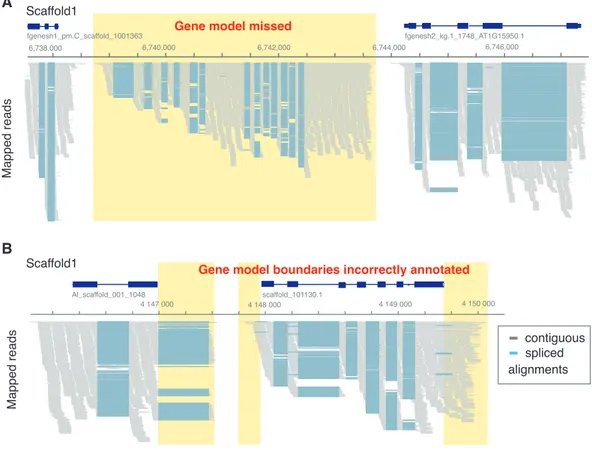
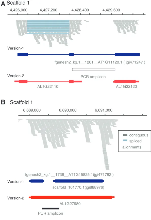
revealed the expected patterns for spliced transcripts indicating instances of unidentified gene models and cases where transcription exceeded known gene boundaries (Figure 2).
Figure 2 | Examples of incorrectly annotated gene models
(A) A gene model was entirely missing, but its locus shows clear evidence of transcription and splicing based on RNA-seq alignments. (B) The boundaries of two gene models do not include the full extent of the transcribed region. In the case of Al_scaffold_001_1048, an entire exon was missing in version-1.
New gene models were predicted from short read alignment data using Cufflinks 2.1.1 (Trapnell et al., 2010) independently for each tissue. In total, Cufflinks predicted 31,194 distinct gene models across all samples. An additional RNA-seq alignment-guided gene
Scaffold1
6,738,000 6,740,000 6,744,000 6,746,000
fgenesh1_pm.C_scaffold_1001363 Gene model missed
fgenesh2_kg.1_1748_AT1G15950.1
4 147 000 4 148 000 4 149 000 4 150 000
Al_scaffold_001_1048 scaffold_101130.1
Mapped readsMapped reads
6,742,000
Gene model boundaries incorrectly annotated
contiguous spliced alignments Scaffold1
A
B
36
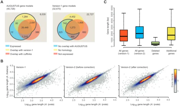
I combined 31,793 Augustus predicted gene models with evidence of transcription or with overlap with version-1 gene models to update the A. lyrata gene annotation (Figure 3). To ensure that I was not excluding any true gene models in version-1, I included 1,430 version-1 gene models with no overlap to any of the new gene models, but showed either evidence of expression or featured an ortholog in at least one of the Brassicaceae species Arabidopsis (The Arabidopsis Genome Initiative, 2000), Capsella rubella (C. rubella) (Slotte et al., 2013), Brassica rapa (B. rapa) (Wang et al., 2011), Schrenkiella parvula (S.
parvula) (Dassanayake et al., 2011) and Arabis alpina (A. alpina) (Willing et al., 2015) (Figure 4A). This step increased the number of gene models to 33,223 (see Materials and Methods). To identify and correct cases where incorrect gene models might have been introduced into the version-2 annotation, I utilized the very close phylogenetic relationship between A. lyrata, Arabidopsis and C. rubella. I compared all gene models that were considerably different between version-1 and version-2 to Arabidopsis and C.
rubella orthologs (see Materials and Methods). If the length of the version-1 open reading frame was closer to that of the orthologs, I retained the version-1 gene model.
This resulted in 548 version-2 gene models being replaced with 688 of the original
version-1 gene models (Figure 4B). After additional step for removal of redundant gene
models, I obtained a final set of 33,221 non-redundant gene models.
Figure 3 | Workflow for RNA-seq incorporation for version-2 annotation
Based on a recent annotation of A. lyrata TEs (Haudry et al., 2013) and sequence similarity to TE genes of Arabidopsis (Lamesch et al., 2012), I annotated 2,089 gene models as TE protein coding genes (see Materials and Methods). Without these, version-2 comprised of 31,132 gene models, which is ~13% more than genes count in Arabidopsis (Lamesch et al., 2012). Although, transfer RNA (tRNA) genes were described in the original analysis of the A. lyrata genome (Hu et al., 2011), version-1 lacks information regarding these loci. By rerunning tRNAScan (Lowe & Eddy, 1997), I identified 660 tRNA genes coding for all 20 amino acids. For completeness, I also incorporated 170 recently published micro RNA (miRNA) genes into the version-2 annotation file (Fahlgren et al., 2010).
Altogether, I updated the coordinates of 29,141 of the original gene models, removed
BLAT alignment
A. lyrata version-2 GFF file AUGUSTUS gene prediction
GFF file A. lyrata
version-1 GTF
Inflorescence GTF
SAM Cufflink transcript prediction TopHat - Bowtie
alignment
Consensus GTF file
Rosette RNA-seq data
SAM RNA-seq data
Inflorescence RNA-seq data
GTF Rosette
38
total predicted transcripts) for known conserved protein domain using InterProScan software ((Quevillon et al., 2005); (Hunter et al., 2009)).
Figure 4 | Overview of gene model annotation and gene length comparison
(A) Left, version-2 gene models predicted by Augustus. Number of gene models overlapping with version- 1 (yellow), genes predicted with Cufflinks (red), and genes with expression evidence (blue). Right, gene models of the version-1 annotation. Number of models without overlap to version-2 models (yellow), without orthologs in five other Brassicaceae (red), and without significant expression evidence (blue). (B) Correlation of the lengths of A. lyrata gene models with the length of their orthologous gene models in Arabidopsis. Left, A. lyrata version-1 gene models. Correlations using version-1 gene models (left), version-2 gene models before (middle) and after (right) the homology-based correction of gene models. (C) Length distribution of gene models including genes that were removed or newly added in the version-2.
Table 1 | Comparison of version-1 and varsion-2 annotation
# version-1 # version-2
Gene models 32,670 33,221
Predicted transcripts 32,670 35,805
Protein-coding genes 32,670 31,221
TE-coding genes - 2,089
miRNA genes - 170
tRNA genes - 660
Featuring ortholog (in at least one Brassicaceae) 23,996 24,146
(40,728)
Expressed Overlap with version-1 Overlap with cufflinks AUGUSTUS gene models
(32,670)
No overlap with AUGUSTUS
Not expressed No homology
B
Version-1 gene models
A
22,727 8,535
323 742
365 882 1,906 4,452
1,273 12
60
1,310 388 2,691 1,284
26,448
Deleted genes
Additional genes All genes
(version-1) All genes (version-2)
0100020003000400050006000
10
5
ytisned eneG
1
Gene length (bp)
C
2.5 3.0 3.5
2.0 2.5 3.0 3.5 4.0 4.5
4.0 4.5 2.5 3.0 3.5 4.0 4.5 2.5 3.0 3.5
Log10 gene length (A. lyrata)
4.0 4.5
Log10 gene length (A. lyrata) Log10 gene length (A. lyrata)
Log10 gene length (A. thaliana)
Version-1 Version-2 (before correction) Version-2 (after correction)
2.2.2 Validating differences in gene model structure
Even after the above-mentioned homology-based gene length adjustments, I found cases where the corresponding gene models from the two annotations varied drastically in length. This included instances where multiple version-1 gene models were fused to form a single gene model in version-2 or vice versa (Figure 5A and 5B). In total, 161 version- 1 genes were split (accounting for 530 genes in version-2) and 1,729 version-1 gene models were merged (accounting for 775 gene models in version-2).
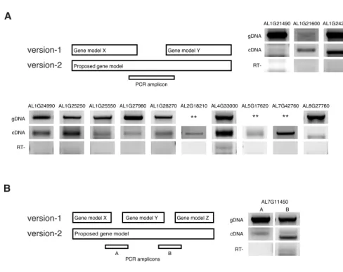
I (in collaboration with Ales Pecinka and Ahmed Abdelsamad) randomly selected 14 version-1 gene models that had been split into multiple gene models in version-2 and 14 gene models that had been merged in version-2 for PCR validation (Figure 6 and 7).
Ales Pecinka and Ahmed Abdelsamad performed PCR validation experiments with
computational support in primer designing from me. For three merge cases, amplification
of genomic DNA (gDNA) failed for primer validation and could not be confirmed. This
was most likely due to large gDNA amplicon size (2.4 – 5 kbp) that rendered the results
of these cases inconclusive. For all 24 remaining cases, PCR results fully confirmed the
annotation of the new gene models.
40
Figure 5 | Examples of wrong split and wrong merge cases in version-1 annotation
(A) Example of a gene model that was split into two gene models in version-2. Reverse transcription-PCR could not confirm the connection of both. (B) Example of version-1 gene models that were merged during the annotation update. Reverse transcription-PCR confirmed presence of a transcript bridging the two version-1 genes.
A
fgenesh2_kg.1__1736__AT1G15825.1(jgi471782 )
B
scaffold_101770.1(jgi888976) AL1G27980
Scaffold 1 Scaffold 1
6,689,000 6,690,000 6,691,000
Version-1
Version-2
PCR amplicon
contiguous spliced alignments Version-1
Version-2 4,426,000
fgenesh2_kg.1__1201__AT1G11120.1 ( jgi471247 ) PCR amplicon
4,427,200 4,428,400 4,429,600
AL1G22110 AL1G22120
Figure 6 | Experimental validation of merged gene models in version-2 annotation
(A) Schematic drawing of two gene models in version-1 that were merged into one in version-2. PCR primers were designed to span regions predicted as intergenic in version-1. gDNA, genomic DNA; cDNA, complementary DNA, RT-, reverse transcription reaction without reverse transcriptase. ** indicate cases where gDNA reaction did not work, most likely due to large amplicon size (2.4 – 5 kb). (B) Validation of version-2 gene model combining three version-1 gene models. The principle follows the description in (A), except that both junctions are validated (A and B).
AL1G21490 AL1G24250
AL1G24990 AL1G25250
AL1G21600
AL1G25550 AL1G27980 AL2G18210 AL5G17620 AL7G42760AL8G27760
AL7G11450 Gene model Y
Gene model X Proposed gene model
version-2
PCR amplicon
Gene model X Proposed gene model
PCR amplicons
A B
** **
A B
B
version-1
Gene model Y Gene model Z
**
A
version-2 version-1
gDNA cDNA RT-
AL1G28270 AL4G33000
gDNA cDNA RT-
gDNA cDNA RT-
jgi317213 jgi318289 jgi887492
AL3G27530 AL3G27520 AL3G12920
AL3G12930 AL1G12890
AL1G12900
jgi861245 AL6G18720 AL6G18710 Proposed gene model Proposed gene model
Gene model X jgi312133 jgi471247
jgi879419 jgi879422
jgi312255
jgi334590 jgi471462
jgi879606 jgi312360 C
A B
amplicon Camplicon C
amplicon Bamplicon A amplicon C
B A
version-2 version-1
PCR amplicons
gDNA cDNA RT-
gDNA cDNA RT-
gDNA cDNA RT- gDNA
cDNA RT-
gDNA cDNA RT-
gDNA cDNA
42
2.2.3 Comparison of version-2 annotation with other Brassicaceae
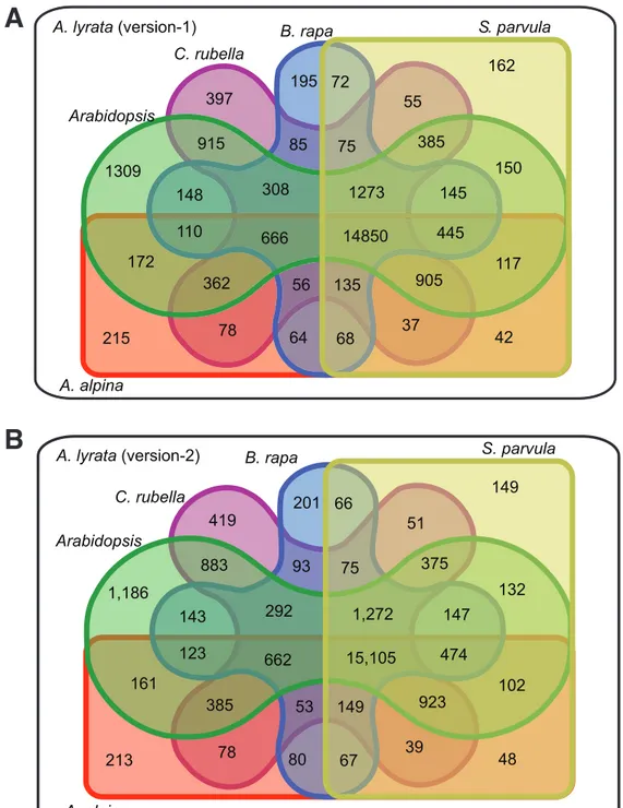
For both A. lyrata annotations, I predicted orthologous relationships between A. lyrata and five other Brassicaceae species (see Materials and Methods). Using version-2 gene models, 77.5% of the genes predicted with an ortholog in at least one species (24,146 out of 31,132) compared to 73% for version-1 (23,996 out of 32,670) (Figure 8A and 8B).
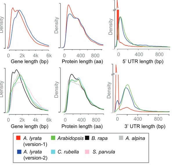
The number of genes with predicted orthologs in all five Brassicaceae was also slightly higher for version-2 with 15,105 genes versus 14,850 genes with version-1. The removal of many short gene models in version-2 changed the distribution of gene model lengths (Figure 9). Version-1 has an excess of gene models shorter than 1 kb with a second peak around 1.5 kb, which describes a bimodal distribution that was only reflected by gene length distribution of B. rapa. In contrast, version-2 had only a single mode around 1.7 kb, similar to the four other species. The length distribution of predicted protein sequences in version-1 was distinct from the other Brassicaceae species, and this discrepancy largely disappeared with version-2. A third factor that contributed to the length differences between the genes of version-1 and version-2 were differences in UTR annotations (Figure 9). In version-1 33% of the genes were annotated without UTR information, however, in version-2 only 5% remained without 3’ and 5’ UTR annotation.
The absolute and relative contributions of individual features are shown in Figure 10.
Though, absolute increase in genomic space for all gene features was observed but CDS
and UTRs benefited the most. I also observed little decrease in intronic genome space,
which can be explained by introduction of splice variants previously missing from
version-1 annotation.
Figure 8 | Comparison of identified orthologs in five Brassicaceae 1309
915 148
150
172
308
362
385
905 1273
117 110
145
56 75 397
85
55
78
195
135 64 37
72
215 42
162
68
445 Arabidopsis
C. rubella
B. rapa S. parvula
A. alpina
666 14850
A. lyrata (version-1)
1,186
883 143
132
161
292
385
375
923 1,272
102 123
147
53 75 419
93
51
78
201
149 80 39
66
213 48
149
67
474 Arabidopsis
C. rubella
B. rapa S. parvula
A. alpina
662 15,105 A. lyrata (version-2)