Complexity Theory WS 2009/10

(1)

Complexity Theory WS 2009/10

Prof. Dr. Erich Grädel

Mathematische Grundlagen der Informatik RWTH Aachen

(2)

cbnd

This work is licensed under:

http://creativecommons.org/licenses/by-nc-nd/3.0/de/

Dieses Werk ist lizensiert uter:

http://creativecommons.org/licenses/by-nc-nd/3.0/de/

http://www.logic.rwth-aachen.de

3 Completeness

3.1 Reductions

Definition 3.1. Let A ⊆ Σ^∗,B ⊆ Γ^∗ be two languages. A function f:Σ^∗→Γ^∗is called areduction from A to Bif, for allx∈Σ^∗,x∈A⇔ f(x)∈B. To put it differently: If f(A)⊆Band f(A^¯) = f(Σ^∗\A) ⊆ (Γ^∗\B) =B. Hence, a reduction from^¯ AtoBis also a reduction from

A¯to ¯B.

Let C be a complexity class (of decision problems). A class of functionsF provides an appropriate notion ofreducibilityforCif

•Fis closed under composition, i.e., if f :Σ^∗→Γ^∗∈ F

and g:Γ^∗→∆^∗∈ F, then g◦f :Σ^∗→∆^∗ ∈ F.

•Cis closed underF: IfB∈ Cand f∈ Fis a reduction fromAto B, thenA∈ C.

For two problemsA,Bwe say thatAisF-deducible toBif there is a function f∈ Fthat is a reduction fromAtoB.

Notation:A≤_F B.

Definition 3.2. A problemBisC-hard underF if all problemsA∈ C areF-reducible toB(A∈ C ⇒A≤_F B).

A problem B is C-complete (underF)ifB ∈ C and B isC-hard (underF).

The most important notions of reducibility in complexity theory are

(4)

3.2 NP-complete problems:Satand variants

•≤_p: polynomial-time reducibility (given by the class of all polynomial-time computable functions)

•≤_log: log-space reducibility (given by the class of functions computable with logarithmic space)

Closure under composition for polynomial-time reductions is easy to show. If

f:Σ^∗→Γ^∗ is computable in timeO(n^k)byMf and g:Γ^∗→∆^∗ is computable in timeO(n^m)byMg,

then there are constantsc,dsuch thatg◦f:Σ^∗→∆^∗is computable in timec·n^k+d(c·n^k)^m=O(n^k+m)by a machine that writes the output ofM_f (whose length is bounded byc·n^k) to a working tape and use it as the input forMg.

In case of log-space reductions this trivial composition does not work sincef(x)can have polynomial length in|x|and hence cannot be completely written to the logarithmically bounded work tape. However, we can use a modified machineM^′_f that computes, for an inputxand a positioni, thei-th symbol of the output f(x). Thus,g(f(x))can be computed by simulating Mg, such that whenever it accesses thei-th symbol of the input, M^′_f is called to compute it. The computation of M^′_f on (x,i) can be done in logarithmic space (space needed for computation and for the counteri: log(n^k)) the symbol f(x,i)written to the tape needs only constant space. Furthermore, the computation of Mgonly needs space logarithmic in the input length asc·log(|f(x)|) = c·log(|x|^k) =c·k·log(|x|) =O(log(|x|)).

3.2 NP-complete problems: Satand variants

NP can be defined as the class of problems decidable in nondeterministic polynomial time:

Definition 3.3. NP=^S_d∈NNtime(n^d).

A different, in some sense more instructive, definition of NP is the class of problems with polynomially-time verifiable solutions:

3 Completeness Definition 3.4. A∈NP if, and only if, there is a problemB∈P and a polynomial psuch thatA={x:∃y(|y| ≤p(|x|)∧x#y∈B)}.

The two definitions coincide: If A has polynomially verifiable solutions viaB∈P and a polynomialp, then the following algorithm decidesAin nondeterministic polynomial time:

Input: x

guessywith|y|<p(n) check whetherx#y∈B

ifanswer is yesthenacceptelsereject

Conversely, let A∈ Ntime(p(n)), and M be a p-time bounded NTM that decidesA. A computation ofMon some input of lengthnis a sequence of at mostp(n)configurations of length≤p(n). Therefore, a computation ofMcan be described by ap(n)×p(n)table with entries fromQ×Σ∪Σand thus by a word of lengthp²(n). Set

B={x#y:yaccepting computation ofMonx}.

We can easily see thatB∈P, andx∈ Lif, and only if, there existsy with|y| ≤p²(n)such thatx#y∈B. Therefore,L∈NP.

Theorem 3.5.

(i) P⊆NP.

(ii)A≤_pB,B∈NP⇒A∈NP.

Clearly NP is closed under polynomial-time reductions:

B∈NP,A≤_pB =⇒ A∈NP.

Bis NP-complete if (1)B∈NP and

(2)A≤pBfor allA∈NP.

The most important open problem in complexity theory isCook’s hypothesis: P̸=NP.

(5)

3.2 NP-complete problems:Satand variants

For every NP-complete problemBwe have:

P̸=NP ⇐⇒ B̸∈P.

We recall the basics of propositional logic. Letτ={X_i:i∈N}be a finite set of propositional variables. The set AL ofpropositional logic formulaeis defined inductively:

(1) 0, 1∈PL (the Boolean constants are formulae).

(2)τ⊆PL (every propositional variable is a formula).

(3) If ψ,ϕ ∈ PL, then also ¬ψ, (ψ∧ϕ), (ψ∨ϕ) and (ψ → ϕ) are formulae in PL.

A(propositional) interpretationis a mapI:σ→ {0, 1}for someσ⊆ τ. It issuitablefor a formulaψ∈PL ifτ(ψ)⊆σ. Every interpretation I that is suitable toψdefines a logical value[[ψ]]^I ∈ {0, 1}with the following definitions:

(1)[[0]]^I:=0, [[1]]^I:=1.

(2)[[X]]^I:=I(X)forX∈σ.

(3)[[¬ψ]]^I:=1−[[ψ]]^I.

(4)[[ψ∧ϕ]]Î:=min([[ψ]]Î,[[ϕ]]Î). (5)[[ψ∨ϕ]]Î:=max([[ψ]]Î,[[ϕ]]Î). (6)[[ψ→ϕ]]Î:= [[¬ψ∨ϕ]]Î.

Amodelof a formulaψ∈PL is an interpretationIwith[[ψ]]^I=1.

Instead of [[ψ]]^I = 1, we will write I |= ψand sayI satisfies ψ. A formulaψis calledsatisfiableif a model for ψexists. A formulaψis called atautologyif every suitable interpretation forψis a model ofψ.

A formulaψis obviously satisfiable iff¬ψis not a tautology. Two formulaeψandϕare called equivalent (ψ≡ϕ) if, for eachI:τ(ψ)∪ τ(ϕ) → {0, 1}, we have [[ψ]]^I = [[ϕ]]^I. A formula ϕfollows fromψ (short,ψ|=ϕ) if, for every interpretationI:τ(ψ)∪τ(ϕ)→ {0, 1}with I(ψ) =1,I(ϕ) =1 holds as well.

Comments. Usually, we omit unnecessary parentheses. As∧and ∨ are semantically associative, we can use the following notations for conjunctions and disjunctions over{ψ_i : i∈I}: ^V_i∈Iψ_irespectively Wi∈Iψi. We fix the set of variablesτ={Xi : i∈N}and encodeXi

3 Completeness byX(bini), i.e., a symbolXfollowed by the binary representation of the indexi. This enables us to encode propositional logic formulae as words over a finite alphabetΣ={X, 0, 1,∧,∨,¬,(,)}.

Definition 3.6. sat:={ψ∈PL :ψis satisfiable}. Theorem 3.7(Cook, Levin). satis NP-complete.

Proof. It is clear thatsatis in NP because {ψ#I|I:τ(ψ)→ {0, 1},I|=ψ} ∈P.

Let Abe some problem contained NP. We show that A≤p sat.

Let M= (Q,Σ,q0,F,δ) be a nondeterministic 1-tape Turing machine decidingAin polynomial timep(n)withF = F⁺∪F⁻. We assume that every computation ofMends in either an accepting or rejecting final configuration, i.e.,Cis a final configuration iff Next(C) =∅. Let w=w0· · ·wn−1 be some input forM. We build a formulaψw∈ PL that is satisfiable iffMaccepts the inputw.

Towards this, letψwcontain the following propositional variables:

•Xq,t forq∈Q, 0≤t≤p(n),

•Y_a,i,tfora∈Σ, 0≤i,t≤p(n),

•Z_i,tfor 0≤i,t≤p(n),

with the following intended meaning:

•Xq,t : “at timet, Mis in stateq,”

•Y_a,i,t: “at timet, the symbolais written on fieldi,”

•Z_i,t: “at timet,Mis at positioni.”

Finally,

ψw:=start∧compute∧end with

start:=X_q₀_,0∧ⁿ⁻¹^{^}

i=0

Y_w_i_,i,0∧

p(n)^ i=n

Y_,i,0∧Z_0,0 compute:=nochange∧change

(6)

3.2 NP-complete problems:Satand variants nochange:= ^{^}

t<p(n),a∈Σ,i̸=j

(Z_i,t∧Y_a,j,t→Y_a,j,t+1) change:= ^{^}

t<p(n),i,a,q

(Xq,t∧Y_a,i,t∧Z_i,t)→

_

(q′,b,m)∈δ(q,a) 0≤i+m≤p(n)

(X_q^′,t+1∧Y_b,i,t+1∧Z_i+m,t+1) end:= ^{^}

t≤p(n),q∈F⁻

¬Xq,t

Here, start “encodes” the input configuration at time 0.

nochangeensures that no changes are made to the field at the current position.changerepresents the transition function.

It is straightforward to see that the mapw7→ψwis computable in polynomial time.

(1) Letw∈L(M). Every computation ofMinduces an interpretation of the propositional variablesXq,t,Ya,i,t,Zi,t. An accepting computation of M on winduces an interpretation that satisfies ψw. Therefore,ψw∈sat.

(2) LetC= (q,y,p)be some configuration ofM,t≤p(n). Set

conf[C,t]:=Xq,t∧^p(n)^{^}

i=0Y_y_i_,i,t∧Zp,t. Please note thatstart=conf[C0(w), 0]. Thus,

ψw|=conf[C0(w), 0]

holds. For every non-final configurationCofMand allt<p(n), we obtain (because of the subformulacomputeofψw) :

ψw∧conf[C,t]|= ^_

C^′∈Next(C)

conf[C^′,t+1].

(3) LetI(ψw) =1. From(1)and(2) it follows that there is at least one computationC0(w) = C0,C1, . . . ,Cr =CendofMonwwith

3 Completeness r≤p(n)such thatI(conf[Ct,t]) =1 for eacht=0, . . . ,v. Further- more,ψw|=¬conf[C,t]holds for all rejecting final configurations CofMand alltbecause of the subformula END ofψw. Therefore, C_endis accepting, andMaccepts the inputw.

We have thus shown thatψw∈satif, and only if,w∈A. q.e.d.

Remark. The reductionw7→ψwis particularly easy; it is computable withlogarithmic space.

A consequence from Theorem 3.7 is thatsatis NP-complete via Logspace-reductions.

Even thoughsatis NP-complete, the satisfiability problem may still be polynomially solvable for some interesting formulae classes S⊆PL. We show that for certain classesS⊆PL,S∩sat∈P while in other casesS∩satis NP-complete.

Reminder. A literal is a propositional variable or its negation. A formulaψ∈PL is indisjunctive normal form (DNF)if it is of the form ψ=^W_i=1ⁿ ^V^m_j=1ⁱ Yij, whereYijare literals. A formulaψis inconjunctive normal form (CNF)if it has the formψ=^Vⁿ_i=1^W^m_j=1ⁱ Y_ij. A disjunction WjY_ijis also calledclause. Every formula ψ∈ PL is equivalent to a formulaψDin DNF and to a formulaψCin CNF.

ψ≡ψD:= ^_

I:τ(ψ)→{0,1}

I(ψ)=1

^ X∈τ(ψ)

X^I

with X^I=





X ifI(X) =1

¬X ifI(X) =0 , and analogously for CNF.

The translationsψ7→ ψ_D,ψ7→ψ_Care computable but generally not in polynomial time. The formulaeψDandψ_Ccan be exponentially longer thanψas there are 2^|τ(ψ)|possible mapsI:τ(ψ)→ {0, 1}.

sat-dnf:={ψin DNF : ψsatisfiable}and

(7)

3.3 P-complete problems

sat-cnf:={ψin CNF : ψsatisfiable}

denote the set of all satisfiable formulae in DNF and CNF, respectively.

Theorem 3.8. sat-dnf∈Logspace⊆P.

Proof. ψ=^W_i^V^m_j=1ⁱ Y_ijis satisfiable iff there is anisuch that no variable in{Y_ij:j=1, . . . ,m_i}occurs both positively and negatively. q.e.d.

Theorem 3.9. sat-cnfis NP-complete via Logspace-reduction.

Proof. The proof follows from the one of Theorem 3.7. Consider the formula

ψw=start∧compute∧end.

From the proof, we see thatstartandendare already in CNF. The same is true for the subformulanochangeofcompute, onlychange is left.changeis a conjunction of formulae that have the form

α:X∧Y∧Z→ ^_^r

j=1Xj∧Yj∧Zj.

Here,r ≤max_(q,a)|δ(q,a)|is fixed, i.e., independent ofnandw. But we have

α≡(X∧Y∧Z→ ^_^r

j=1

U_j)∧^{^}^r

j=1

(U_j→X_j)∧(U_j→Y_j)∧(U_j→Z_j)).

Therefore,A≤_logsat-cnffor eachA∈NP. q.e.d.

A (propositional)Horn formulais a formulaψ=^V_i^W_jY_i_jin CNF where every disjunction^W_jY_jcontains at most one positive literal. Horn formulae can also be written as implications by the following equivalences:

¬X1∨ · · · ∨ ¬Xk∨X≡(X1∧ · · · ∧Xk)→X,

¬X1∨ · · · ∨ ¬X_k≡(X1∧ · · · ∧X_k)→0.

3 Completeness Lethorn-sat={ψ∈PL : ψa satisfiable Horn formula}. We know from mathematical logic:

Theorem 3.10. horn-sat∈P.

This follows, e.g., by unit resolution or the marking algorithm.

Theorem 3.11. horn-satis P-complete via logspace reduction.

Proof. Let A∈ Pand Ma deterministic 1-tape Turing machine, that decidesAin timep(n). Looking at the reductionw 7→ψwfrom the proof of Theorem 3.7, we see that the formulaestart,nochangeand endare already Horn formulae. SinceMwas chosen to be deterministic, i.e.,|δ(q,a)|=1,changetakes the form(X∧Y∧Z)→(X^′∧Y^′∧Z^′). This is equivalent to the Horn formula(X∧Y∧Z) →X^′∧(X∧Y∧ Z) →Y^′∧(X∧Y∧Z) → Z^′. We thus have a logspace computable functionw7→ψbwsuch that

•ψbwis a Horn formula,

•Macceptswiffψbwis satisfiable.

Therefore,A≤_loghorn-sat. q.e.d.

Another fundamental P-complete problem is the computation of winning regions in finite (reachability) games.

Such a game is given by a game graphG= (V,V0,V1,E)with a finite setVof positions, partitioned intoV₀andV₁, such that Player 0 moves from positionsv∈V0, moves from positionsv∈V₁. All moves are along edges, and we use the term playto describe a (finite or infinite) sequence v₀v₁v₂. . . with (v_i,v_i+1) ∈ E for all i. We use a simple positional winning condition: Move or lose! Playerσwins at positionvifv∈V1−σandvE=∅, i.e., if the position belongs to the opponent and there are no possible moves possible from that position.

Note that this winning condition only applies to finite plays, infinite plays are considered to be a draw.

Astrategyfor Playerσis a mapping f :{v∈Vσ:vE̸=∅} →V

with(v,f(v))∈Efor allv∈V. We call f winningfrom positionvif all plays that start atvand are consistent with f are won by Playerσ.

(8)

We now can definewinning regions W0andW₁:

Wσ={v∈V: Playerσhas a winning strategy from positionv}. This leads to several algorithmic problems for a given gameG:

The computation of winning regionsW0andW₁, the computation of winning strategies, and the associated decision problem

game:={(G,v): Player 0 has a winning strategy forGfromv}. Theorem 3.12. gameis P-complete and decidable in time O(|V|+|E|).

A simple polynomial-time approach to solvegameis to compute the winning regions inductively:Wσ=^S_n∈NW_σⁿ, where

W_σ⁰={v∈V1−σ:vE=∅}

is the set of terminal positions which are winning for Playerσ, and W_σⁿ⁺¹={v∈Vσ:vE∩W_σⁿ̸=∅} ∪ {v∈V1−σ:vE⊆W_σⁿ} is the set of positions from which Playerσcan win in at mostn+1 moves.

Aftern ≤ |V|steps, we have thatW_σⁿ⁺¹ =W_σⁿ, and we can stop the computation here.

To solvegamein linear time, use the slightly more involved Algo- rithm 3.1. Procedure Propagate will be called once for every edge in the game graph, so the running time of this algorithm is linear with respect to the number of edges inG.

The problemgameis equivalent to the satisfiability problem for propositional Horn formulae. We recall that propositional Horn formulae are finite conjunctions^V_i∈IC_iof clausesC_iof the form

X1∧. . .∧Xn → X or X₁∧. . .∧Xn

| {z }

body(Ci)

→ |{z}0

head(Ci)

.

A clause of the formXor 1→Xhas an empty body.

3 Completeness Algorithm 3.1.A linear time algorithm forgame

Input: A gameG = (V,V₀,V₁,E) Output: Winning regionsW0andW1

foreachv∈Vdo /* 1: Initialisation */

win[v]:=⊥ P[v]:=∅ n[v]:=0 endfor

foreach(u,v)∈Edo /* 2: Calculate P and n */

P[v]:=P[v]∪ {u} n[u]:=n[u] +1 endfor

foreachv∈V0do /* 3: Calculate win */

ifn[v] =0thenPropagate(v, 1) endfor

foreachv∈V\V0do

ifn[v] =0thenPropagate(v, 0) endfor

returnwin

procedurePropagate(v,σ) ifwin[v]̸=⊥thenreturn

win[v]:=σ /* 4: Mark v as winning for player σ */

foreachu∈P[v]do /* 5: Propagate change to predecessors */

n[u]:=n[u]−1ifu∈Vσor n[u] =0thenPropagate(u,σ) endfor

We will show thatsat-hornandgameare mutually reducible via logspace and linear-time reductions.

(1)game≤_log-linsat-horn

For a game G = (V,V₀,V₁,E), we construct a Horn formulaψG

with clauses

v→u for allu∈V0and(u,v)∈E, and v₁∧. . .∧vm→u for allu∈V₁anduE={v₁, . . . ,vm}. The minimal model of ψG is precisely the winning region of Player 0, so

(G,v)∈game ⇐⇒ ψG∧(v→0)is unsatisfiable.

(9)

3.4 NLogspace-complete problems

(2)sat-horn≤_log-lingame

For a Horn formulaψ(X₁, . . . ,Xn) = ^V_i∈IC_i, we define a game G_ψ= (V,V0,V1,E)as follows:

V={0} ∪ {X₁, . . . ,Xn}

| {z }

V0

∪ {C_i:i∈ I}

| {z }

V1

and

E={X_j→C_i:X_j=head(C_i)} ∪ {C_i→X_j:X_j∈body(C_i)}, i.e., , Player 0 moves from a variable to some clause containing the variable as its head, and Player 1 moves from a clause to some variable in its body. Player 0 wins a play if, and only if, the play reaches a clauseCwith body(C) =∅. Furthermore, Player 0 has a winning strategy from positionXif, and only if,ψ|=X, so we have

Player 0 wins from position 0 ⇐⇒ ψis unsatisfiable.

In particular, gameis P-complete, and sat-horn is solvable in linear time.

We already know that the reachability problem, i.e. to decide, given a directed graphGand two nodesaandb, whether there is a path from atobinG, is in NLogspace.

Theorem 3.13. reachabilityis NLogspace-complete.

Proof. LetAbe an arbitrary problem in NLogspace. There is a nondeterministic Turing machineMthat decidesAwith workspaceclogn.

We prove thatA≤_logreachabilityby associating, with every input xfor M, a graphGx = (Xx,Ex)and two nodesaandb, such thatM acceptsxif, and only if, there is a path fromatobinGx. The set of nodes ofGxis

Vx:={C:Cis a partial configuration of Mwith

workspaceclog|x|} ∪ {b},

3 Completeness

and the set of edges is

Ex:={(C,C^′):(C,x)⊢_M(C^′x)} ∪ {(Ca,b):Cais accepting}. Recall that a partial configuration is a configuration without the descrip- tion of the input. Each partial configuration inVxcan be described by a word of lengthO(log|x|). Further we defineato be the initial partial configuration ofM. Clearly(Gx,a,b)is constructible with logarithmic space fromxand there is a path fromatobinGx if, and only if, there

is an accepting computation ofMonx. q.e.d.

We next discuss a variant ofsatthat is NLogspace-complete.

Definition 3.14. A formula is inr-CNF if it is in CNF and every clause contains at mostrliterals:ψ=^Vⁿ_i=1^W^m_j=1ⁱ Y_i_j withm_i≤rfor alli.

Furthermore,r-sat:={ψinr-CNF : ψis satisfiable}. It is known thatr-satis NP-complete for allr≥3.

To the contrary, 2-satcan be solved in polynomial time, e.g., by resolution:

• The resolvent of two clauses with≤2 literals contains at most 2 literals.

• At mostO(n²) clauses with≤ 2 literals can be formed with n variables.

Hence, we obtain that Res^∗(ψ)for a formulaψin 2-CNF can be computed in polynomial time. One can show an even stronger result.

Theorem 3.15. 2-satis in NLogspace.

Proof. We show that {ψ : ψin 2-CNF,ψunsatisfiable} ∈ NLogspace.

Then, by the Theorem of Immerman and Szelepcsényi, also 2-sat ∈ NLogspace. The reduction maps a formulaψ∈2-CNF to the following directed graphGψ= (V,E):

•V={X,¬X:X∈τ(ψ)}represents the literals ofψ.

•E={(Y,Z):ψcontains a clause equivalent to(Y→Z)}.

(10)

X1 X2 X3

¬X1 ¬X2 ¬X3 (a)Gψa

X1 X2

¬X1 ¬X2 (b)Gψb

Figure 3.1.Graphs forψa=X1∧(¬X1∨X2)∧(X3∨ ¬X2)∧(¬X3∨ ¬X1)and ψb= (X1∨X2)

Example3.16. Figures 3.1(a) and 3.1(b) show the graphs constructed for an unsatisfiable and a satisfiable 2-CNF formula, respectively.

Lemma 3.17(Krom-Criterion). Letψbe in 2-CNF.ψis unsatisfiable if, and only if, there exists a variableX∈τ(ψ)such thatGψcontains a path fromXto¬Xand one from¬XtoX.

The problem

L={(G,a,b):Gdirected graph, there is a path fromatob} is also called the labyrinth problem. A formulaψis unsatisfiable if, and only if, there exists a variableX∈τ(ψ)such that(Gψ,X,¬X)∈Land (Gψ,¬X,X)∈L. SinceL∈NLogspace, the claim follows. q.e.d.

Proof (of Lemma 3.17). We use the notationY→^∗_ψZto denote that there exists a path fromYtoZinGψ.

Let I be an interpretation such that I(ψ) = 1. Then, I(Y) = 1,Y →^∗_ψ Z =⇒ I(Z) = 1. Hence, if X →^∗_ψ ¬X →^∗_ψ X, then ψis unsatisfiable.

Conversely, for allX∈τ(ψ), either notX→^∗_ψ¬Xor not¬X→^∗_ψX.

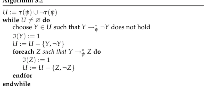
In this case, Algorithm 3.2 constructs an interpretationI such that I(ψ) =1.

It is not possible to produce conflicting assignments resulting from Y→^∗_ψZas well asY→^∗_ψ ¬Zsince this would imply¬Z→^∗_ψ¬Yand Z→^∗_ψ¬Y, and henceY→^∗_ψZ→^∗_ψ¬Y. ButYwas chosen as to not have this property.

3 Completeness

Algorithm 3.2 U:=τ(ψ)∪ ¬τ(ψ) whileU̸=∅do

chooseY∈Usuch thatY→^∗_ψ¬Ydoes not hold I(Y):=1

U:=U− {Y,¬Y}

foreachZ such that Y→^∗_ψZdo I(Z):=1

U:=U− {Z,¬Z} endfor

endwhile

Thus, Algorithm 3.2 constructs an interpretationIsince, for every variableX∈τ(ψ), eitherI(X) =1 orI(¬X) =1. However, due to the nondeterministic choice ofYin each loop, the resulting interpretation is not uniquely determined.

LetIbe an interpretation constructed by Algorithm 3.2. It remains to prove thatIsatisfies each clause(Z∨Z^′), and thusψ.

Otherwise, there is a clause(Z∨Z^′)such thatI(Z) =I(Z^′) =0, i.e.,I(¬Z) =1. This implies, that the algorithm has chosen a literalY such thatY→^∗_ψ¬ZbutY→^∗_ψ¬Ydoes not hold. Since¬Z→^∗_ψZ^′, we obtainY→^∗_ψZ^′and henceI(Z^′) =1, which is a contradiction. q.e.d.

Remark3.18. Formulae in 2-CNF are sometimes calledKrom-formulae.

Theorem 3.19. 2-satis NLogspace-complete.

Proof. We prove thatreachability≤_log2-sat.

Given a directed graphG= (V,E)with nodesaandb, we construct the 2-CNF formula

ψ_G,a,b:=a∧ ^{^}

(u,v)∈E

(u→v)∧ ¬b.

Clearly this defines a logspace-reduction from the reachability

problem to 2-sat. q.e.d.

(11)

3.5 APspace-complete problem

3.5 A Pspace-complete problem

Let us first recall two important properties of the complexity class Pspace:=^S_kDspace(n^k).

• Pspace=^S_k∈NNspace(n^k) =NPspacebecause, by the Theorem of Savitch, Nspace(S)⊆Dspace(S²).

• NP ⊆Pspacesince Ntime(n^k) ⊆Nspace(n^k) ⊆ Dspace(n^2k) ⊆ Pspace.

A problemAis Pspace-hard ifB ≤_p Afor allB∈Pspace. Ais Pspace-complete if A∈PspaceandAis Pspace-hard.

As an example of Pspace-complete problems, we consider the evaluation problem for quantified propositional formulae (also called QBF for “quantified Boolean formulae”).

Definition 3.20. Quantified propositional logicis an extension of (plain) propositional logic. It is the smallest set closed under disjunction, conjunction and complement that allows quantification over propositional variables in the following sense: Ifψis a formula from quantified propositional logic andXa propositional variable, then∃Xψ,∀Xψare also quantified propositional formulae.

Example3.21. ∃X(∀Y(X∨Y)∧ ∃Z(X∨Z)).

By free(ψ)we denote the set of free propositional variables inψ.

Every propositional interpretationI:σ→ {0, 1}withσ⊆τdefines logical valuesI(ψ) for all quantified propositional formulaeψwith free(ψ) ⊆ σ. LetI be an interpretation andX ∈ τ a propositional variable. Further, we writeI[X=1]for the interpretation that agrees withIon allY∈ τ,Y̸=Xand interpretsXwith 1. Analogously, let I[X=0]be the interpretation withI[X/0](Y) =I(Y)forY̸=Xand I[X/0](X) =0. Then,I(∃Xψ) =1 if, and only if,I[X/0](ψ) =1 or I[X/1](ψ) =1. Similarly,I(∀Xψ) =1 if, and only if,I[X/0](ψ) =1 andI[X/1](ψ) =1.

Observe that if free(ψ) = ∅ the value I(ψ) ∈ {0, 1} does not depend on a concrete interpretationI; we have eitherI(X) =1 (ψis satisfied) orI(X) = 0 (ψisunsatisfied). The formula∃X(∀Y(X∨Y)∧

∃Z(X∨Z))is satisfied, for example.

3 Completeness Algorithm 3.3.Eval(ψ,I)

Input: ψ,I

ifψ=X∈VthenreturnI(X) ifψ= (ϕ1∨ϕ2)then

ifEval(ϕ1,I) =1thenreturn 1elsereturn Eval(ϕ2,I) endif

ifψ= (ϕ1∧ϕ2)then

ifEval(ϕ₁,I) =0thenreturn 0elsereturn Eval(ϕ₂,I) endif

ifψ=¬ϕthenreturn 1−Eval(ϕ,I) ifψ=∃Xϕthen

ifEval(ϕ,I[X=0]) =1thenreturn 1else return Eval(ϕ,I[X=1])

endif endif

ifψ=∀Xϕthen

ifEval(ϕ,I[X=0]) =0thenreturn 0else return Eval(ϕ,I[X=1])

endif endif

Definition 3.22.

qbf:={ψa quantified PL formula : free(ψ) =∅, ψtrue}. Remark3.23. Letψ=ψ(X₁, . . . ,Xn)be a propositional formula (i.e., one that does not contain quantifiers). Then,

ψ∈sat ⇐⇒ ∃X1. . .∃Xnψ∈qbf.

qbfis therefore at least as hard assat. Actually, we will show thatqbf is Pspace-complete.

Theorem 3.24. qbf∈Pspace.

Proof. The recursive procedure Eval(ψ,I)presented in Algorithm 3.3 computes the valueI(ψ)for a quantified propositional formulaψand I: free(ψ)→ {0, 1}.

This procedure usesO(n²) space. It is easy to see thatI(ψ) is

computed correctly. q.e.d.

(12)

3.5 APspace-complete problem

Theorem 3.25. qbfis Pspace-hard.

Proof. Consider a problem Ain Pspace and letMbe some n^k-space bounded 1-tape TM with L(M) = A. Every configuration of M on some inputwof lengthncan be described by a tuple ¯Xof propositional variables consisting of:

Xq (qis state ofM) : “Mis in stateq”, X^′_a,i (atape symbol,i≤n^k) : “symbolais on fieldi”, X^′′_j (j≤n^k) : “Mis on positionj”.

As in the NP-completeness proof forsat, we construct formu- laeconf(X^¯), next(X, ¯^¯ Y), inputw(X^¯)andacc(X^¯)with the following intended meanings:

•conf(X^¯): ¯Xencodes some configuration, i.e., exactly oneXqis true, exactly oneX^′_a,iis true for everyi, and exactly oneX^′′_j is true.

•inputw(X^¯) : ¯X encodes the initial configuration of M on w = w0. . .wn−1:

inputw(X^¯):=conf(X^¯)∧Xq0∧ⁿ⁻¹^{^}

i=0X_w^′_i_,i∧ ⁿ

^k

i=nX^′_,i∧X₀^′′.

•acc(X^¯): ¯Xis an accepting configuration:

acc(x¯):=conf(X^¯)∧ ^_

q∈E⁺

Xq.

•next(X, ¯^¯ Y): ¯Yis a successor configuration of ¯X:

next(X, ¯^¯ Y):=^{^}

i

X^′′_i → ^{^}

a,j̸=i

(Y_a,j^′ ↔Xa,j)∧

^

δ(q,a)=(q′,b,m) 0≤m+i≤nk

(Xq∧X^′_a,i→Y_q^′∧Y_b,i^′ ∧Y_i+m^′′ ).

Givenw, these formulae can be constructed in polynomial time.

3 Completeness

Furthermore, we define the predicate eq(X, ¯^¯ Y):=^{^}

q(Xq↔Yq)∧^{^}

a,i

(X^′_a,i↔Y_a,i^′ )∧^{^}

j

(X^′′_j ↔Y_j^′′).

We inductively construct formulaereachm(X, ¯^¯ Y)expressing that ¯Xand Y¯ encode configurations and ¯Yis accessible from ¯Xin at most 2^msteps.

Form=0, let

reach0(X, ¯^¯ Y):=conf(X^¯)∧conf(Y^¯)∧(eq(X, ¯^¯ Y)∨next(X, ¯^¯ Y)). A naïve way to definereachm+1would be

reachm+1(X, ¯^¯ Y):=∃Z^¯(reachm(X, ¯^¯ Z)∧reachm(Z, ¯^¯ Y)).

reachm+1(X, ¯^¯ Y):=

∃Z^¯∀U^¯∀V^¯ (eq(X, ¯^¯ U)∧eq(Z, ¯^¯ V))

∨(eq(Z, ¯^¯ U)∧eq(Y, ¯^¯ V))

!

→reachm(U, ¯^¯ V).

We now obtain:

|reach0|=O(n^k)for some appropriatek, and

IfMaccepts the inputwusing spacen^kit performs at most≤2^c·n^k steps for some constantc. Setm:=c·n^kand

ψw:=∃X^¯ ∃Y^¯(input(X^¯)∧acc(Y^¯)∧reachm(X, ¯^¯ Y)).

Obviously,ψwis constructable fromwin polynomial time andψw∈qbf if and only ifw∈L(M). Therefore,qbfis Pspace-complete. q.e.d.

Complexity Theory WS 2009/10