Complex Langevin simulation of a random matrix model at nonzero chemical potential

JHEP03(2018)015

Published for SISSA by Springer

Received: December 26, 2017 Accepted: January 24, 2018 Published: March 6, 2018

Complex Langevin simulation of a random matrix model at nonzero chemical potential

J. Bloch,

J. Glesaaen,

J.J.M. Verbaarschot

and S. Zafeiropoulos

aInstitute for Theoretical Physics, University of Regensburg, 93040 Regensburg, Germany

bDepartment of Physics, Swansea University, Swansea, U.K.

cDepartment of Physics and Astronomy, Stony Brook University, Stony Brook, NY 11794, U.S.A.

dInstitute for Theoretical Physics, Heidelberg University, Philosophenweg 12, 69120 Heidelberg, Germany

eDepartment of Physics, The College of William & Mary, Williamsburg, VA 23187, U.S.A.

fThomas Jefferson National Accelerator Facility, Newport News, VA 23606, U.S.A.

E-mail: jacques.bloch@ur.de, jonas.glesaaen@swansea.ac.uk, jacobus.verbaarschot@stonybrook.edu,

zafeiropoulos@thphys.uni-heidelberg.de

Abstract: In this paper we test the complex Langevin algorithm for numerical simulations of a random matrix model of QCD with a first order phase transition to a phase of finite baryon density. We observe that a naive implementation of the algorithm leads to phase quenched results, which were also derived analytically in this article. We test several fixes for the convergence issues of the algorithm, in particular the method of gauge cooling, the shifted representation, the deformation technique and reweighted complex Langevin, but only the latter method reproduces the correct analytical results in the region where the quark mass is inside the domain of the eigenvalues. In order to shed more light on the issues of the methods we also apply them to a similar random matrix model with a milder sign problem and no phase transition, and in that case gauge cooling solves the convergence problems as was shown before in the literature.

Keywords: Lattice QCD, Lattice Quantum Field Theory, Matrix Models

ArXiv ePrint: 1712.07514

JHEP03(2018)015

Contents

1 Introduction 1

2 Random matrix model 3

3 Complex Langevin 7

4 The Dirac spectrum and the fermion determinant 10

5 Reweighted complex Langevin 12

6 Shifted representation 16

7 Gauge cooling 18

7.1 Cooling norms 18

7.2 Computing h 19

7.3 Results 20

8 Deformation technique 23

9 Conclusions 25

A The phase quenched partition function 27

A.1 Solution for the condensed phase 28

A.2 Normal phase 29

A.3 Free energy 29

1 Introduction

A first principles study of the QCD phase diagram in the plane of temperature (T ) and

baryon chemical potential (µ) is one of the most challenging problems of modern high

energy physics. Its understanding will lead to profound answers ranging from cosmology

and the early universe to the physics of neutron stars. Analytical approaches tend to fail

because the theory is strongly interacting, and only for extreme values of the temperature

and/or the baryon chemical potential can the theory be studied perturbatively due to

asymptotic freedom. Lattice numerical simulations have contributed tremendously to the

understanding of the vacuum properties of the theory and have also firmly established that

with physical quark masses the deconfinement transition at zero baryon chemical potential

is a crossover. Despite all these celebrated results the situation at finite baryon density

is very different [1] and our knowledge is mainly based on models for QCD or lattice

simulations at small values of µ (more precisely µ/T < 1 and µ < m

/2 [2]).

JHEP03(2018)015

It is well known that the culprit behind this lack of results is the infamous sign problem which is prohibiting numerical simulations when µ/T > 1 or µ > m

/2. The determinant of the Dirac operator becomes complex for SU(N

) Yang-Mills theories with N

≥ 3 and quarks in the fundamental representation. Consequently, standard Markov Chain Monte Carlo (MCMC) methods, which require a real and positive probability weight, cannot be applied. There have been many attempts at tackling this problem by the QCD community.

Some of them try to circumvent the sign problem, while others study related theories which have no sign problem. To circumvent the sign problem one can perform a Taylor expansion around µ = 0 [3] or use reweighting methods [4], however, these methods cannot go beyond µ/T ≥ 1 at physical quark masses due to serious problems such as the limited radius of convergence of the Taylor series or the exponentially small reweighting factor. Alterna- tively, one can study QCD with imaginary baryon chemical potential [5, 6], or perform simulations of two-color QCD or of QCD with adjoint quarks [3, 7, 8], which have no sign problem at all. However, as these theories have a different phase diagram from the one of QCD, one can at best extract qualitative information regarding the QCD phase diagram.

A method that has attracted a great deal of attention recently, and which is not based on MCMC methods, is the method of stochastic quantization, also called Langevin method.

For the case of complex actions, the complex Langevin (CL) method was pioneered indepen- dently by Parisi [9] and Klauder [10] more than 30 years ago. Despite the fact that stochas- tic quantization yields the same results as path integral quantization for systems with a real action, this is, unfortunately, not always the case when the action is complex. One of the most serious problems is that the method sometimes converges towards the wrong limit.

Convergence criteria have been established [11], however, these are not fulfilled in realistic QCD simulations, at least for the range of parameters that are of interest for mapping the unknown part of the QCD phase diagram [12, 13]. Nevertheless, the CL algorithm has given correct results in many non-trivial systems for which we know the solution, and it seems to be quite successful for QCD simulations in the deconfined phase [12, 13], as well as in simulations for heavy quarks [14–17], where the results can be validated by other methods.

In this article we are attempting to understand the properties of the algorithm very close to the chiral limit in the cold and dense regime. To achieve that, we are studying a random matrix theory (RMT) model which shares many key features of QCD such as spontaneous breaking of chiral symmetry, a finite density phase transition, as well as a complex fermion determinant, which causes a strong sign problem. The model that we have been studying was introduced by Stephanov [18] based on a random matrix model for the finite temperature chiral phase transition [19]. There is a significant literature studying the convergence properties of the CL algorithm in RMT but all the existing studies are based on a finite density model introduced by Osborn [20] (or an improved version thereof [21]), which possesses many similarities with the one by Stephanov but also has big differences, most notably the lack of a phase transition to a nonzero baryon density phase. Sensu stricto the Osborn model is only a model of QCD in the confined phase at small chemical potential.

A great deal of analytical knowledge for non-perturbative aspects of QCD came from

RMT studies. These include among others finite density results [22], lattice spacing effects

on the lowest eigenvalues of the Dirac operator for Wilson fermions [23–28], and the effect

JHEP03(2018)015

of topology on the Dirac spectrum [29]. In this article we are addressing the convergence properties of the CL algorithm for a model of continuum QCD at nonzero chemical poten- tial. The model has a known analytic solution, and by simulating it numerically we can get an explicit handle on the various issues of the algorithm.

This article starts out with the definition of the random matrix models that will be studied by the CL algorithm which is introduced in section 3. In section 4, we discuss the fermion determinant and the spectrum of the Dirac operator. The CL reweighting method is analyzed in section 5, while the shifted representation, in which the chemical potential is shifted to the bosonic part of the action, is discussed in section 6. Cooling methods are investigated for two different random matrix models in section 7. As a last attempt to fix the convergence problems of the CL algorithm, we study the deformation method in section 8. Concluding remarks are made in section 9, and analytical results for the phase quenched partition function are worked out in appendix. A preliminary account of some of the results in this paper appeared as conference proceedings [30, 31].

2 Random matrix model

In this section we discuss a random matrix theory inspired model [19, 32] for QCD at finite baryon density originally proposed by Stephanov [18]. The model’s partition function reads

Z

= e

Z

dW dW

det

(D + m)e

. (2.1) The Dirac operator D has the form

D = 0 iW + µ iW

+ µ 0

!

, (2.2)

where a term containing the baryon chemical potential µγ

has been coupled to the chRMT Dirac operator proposed in [29, 32]. The N × (N + ν) matrix elements of W are complex numbers, N is the size of the block matrix W and the index ν of the Dirac Matrix is the analogue of the topological charge. This model was first introduced for imaginary chemical potential [19] to study the QCD chiral phase transition at nonzero temperature (which in the model appears as an imaginary chemical potential).

In this article we choose ν = 0, since the topological charge does not have a significant effect on the quantities of interest. For µ > 0, the eigenvalues of D become complex, and are roughly distributed homogeneously inside a strip of width ∼ µ

(for finite N it is an ellipse). Similarly to QCD, numerical simulations of this random matrix theory have an exponentially hard sign problem, especially when the quark mass is inside the cloud of eigenvalues of the Dirac operator.

Our attention will be focused mainly on two observables, the mass dependent chiral condensate (note that the physical chiral condensate is − Σ) defined by

Σ = 1 2N

∂ log Z

∂m , (2.3)

JHEP03(2018)015

and the baryon number density given by n

= 1

2N

∂ log Z

∂µ . (2.4)

There is no unique way of introducing a chemical potential in a random matrix model. Some alternatives turn to be advantageous from a symmetry point of view [20]. In particular, the Osborn model [20] has a U(N ) × U(N ) symmetry which makes it possible to obtain analytical results for the joint probability distribution function of the eigenvalues, which is the starting point of many powerful random matrix methods. The Stephanov model has only a U(N ) invariance, and it is not possible to obtain an analytical solution for the joint eigenvalue density. In the case of the Osborn model, by extending the method of orthogonal polynomials to bi-orthogonal polynomials, all n-point spectral correlators can be obtained.

The Osborn model is a two-matrix model that has a form similar to the Stephanov model. In the chiral basis it is given by

Z

= e

Z

dW dW

dW

dW

det

(D + m)e

, (2.5) where the Dirac operator D has the form

D = 0 iW + µW

iW

+ µW

0

!

. (2.6)

Remarkably, the partition function at finite baryon density can be related to the one at zero baryon density by introducing a trivial multiplicative factor and a mass rescaling as follows [20, 33],

Z

(m, µ) = (1 − µ

)

Z

m p 1 − µ

, 0

!

. (2.7)

Consequently, it is natural to expect that the Osborn model does not possess the rich phenomenological structure of the Stephanov model, which exhibits a phase transition sep- arating a phase with zero baryon density from a phase with nonzero baryon density. Strictly speaking the Osborn model should only be considered as a model for QCD at small chemical potential, precisely due to the absence of a phase transition to a phase with nonzero baryon density. In addition, one can conclude that the sign problem of the Osborn model is of a weaker nature and therefore may be remedied by some clever techniques [21, 33–37]. Both random matrix models possess the same global symmetries with the same spontaneous symmetry breaking pattern as in QCD and yield the ε-limit of the QCD chiral Lagrangian.

It is noteworthy that in case of QCD with three colors in the fundamental representation

this chiral Lagrangian does not have a dependence on the baryon chemical potential. The

reason is that the Goldstone bosons, i.e., the pions, do not carry baryon charge. The chiral

Lagrangian of phase quenched QCD, where µ becomes the isospin chemical potential, has

a nontrivial µ-dependence which, at the mean field level, or in the ε-domain, is given by

the µ dependence of the large N limit of the partition functions (2.1) or (2.5).

JHEP03(2018)015

We could contemplate other random matrix models where the dependence of the chem- ical potential is integrated out in the evaluation of the partition function. For example, the Dirac operator

D = 0 iW + µe

iW

+ µe

0

!

, (2.8)

where ϕ is uniformly random in [ − π, π], and the partition function is defined by Z

= e

Z

dϕdW dW

det

(D + m)e

. (2.9) It is clear that the partition function does not depend on µ while the eigenvalues of D are complex. Since the chemical potential can be eliminated by changing the integration contour of the ϕ integral, the CL algorithm should be able to solve this problem correctly.

We will, however, not study this model in this paper.

The unquenched partition function of the Stephanov model was cast analytically in a form that allows for either an easy numerical evaluation at finite N , or that allows for a complete analytical solution via a saddle point approximation in the thermodynamic limit where N → ∞ [18, 22]. For the N

= 1 case, the partition function, in units where the chiral condensate Σ = 1 (here we are referring to the Low Energy Constant of Chiral Perturbation Theory), takes the following σ-model form via bosonization methods

Z

(m, µ) = e

Z

dσdσ

e

(σσ

+ m(σ + σ

) + m

− µ

)

, (2.10) where σ is the bosonized version of ¯ ψ

ψ

. A change of variables to polar coordinates renders the angular integral calculable analytically and yields a modified Bessel function, such that the partition function can be written as a one-fold integral,

Z

(m, µ) = πe

Z

0

du(u − µ

)

I

(2mN √

u)e

. (2.11) A saddle point analysis of the partition function can be performed in the thermody- namic limit. This was analyzed in detail in [22] but we will repeat some of the main steps here for the convenience of the reader. The saddle point equation reads

1

u − µ

= 1 − m

√ u . (2.12)

The Stephanov model exhibits a first order phase transition which takes place when

| Z

| = | Z

| , with u

and u

being two different solutions of the saddle-point equation giving the same free-energy. One can rewrite this condition

| (u

− µ

)e

| = | (µ

− u

)e

| . (2.13) This is a transcendental equation that, in the chiral limit, has the solutions u

= 0 and u

= 1 + µ

. Therefore in this limit one has the critical curve

Re

1 + µ

+ log µ

= 0, (2.14)

JHEP03(2018)015

−2

−1.5

−1

−0.5 0 0.5 1 1.5 2

−2 −1.5 −1 −0.5 0 0.5 1 1.5 2

µ

m

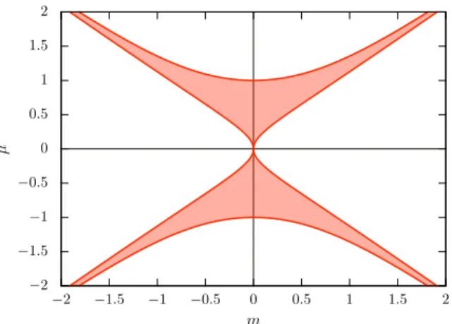
Figure 1. Phase diagram of the two flavor phase quenched random matrix theory in the mass- chemical potential plane. The shaded area shows the region of the phase diagram with a nonzero pion condensate which lies in between the pion condensation transition and a chiral phase transition.

which for the case of a real baryon chemical potential leads to the critical value µ

= 0.527 . . . in the chiral limit. This critical curve is also valid for the case of a complex chemical potential. In particular, for an imaginary chemical potential, there is a second order phase transition to a restored phase at µ = 1.

We will also compare our results to the two-flavor phase quenched RMT partition function [38] or the partition function at nonzero isospin chemical potential [39, 40]. The two-flavor partition function is an eight dimensional integral and is much more complicated than the one-flavor partition function, which is only a two-dimensional integral. However, in the large N limit, it can be evaluated by a saddle-point approximation, see appendix A.

It has a pion-condensation phase for µ > m

/2 corresponding to the parameter domain when the quark mass is inside the support of the eigenvalues. In figure 1 we show the phase diagram in the plane of the chemical potential and quark masses (which are taken to be equal for the two flavors). For nonzero mass and increasing chemical potential, we find a phase transition to a pion condensation phase at µ = m

/2, and for larger µ, a second phase transition to a chirally restored phase. In the region between the curves, the quark mass is in the domain of the eigenvalues and CL is expected to fail. In the outside region, the mean field result for full QCD and phase quenched QCD coincide, and CL is expected to work. For QCD we expect a similar forbidden region.

In order to study the properties of the Langevin algorithm we will perform numerical

simulations of the Stephanov model employing the CL algorithm and test its convergence

properties by comparing the obtained numerical data for the chiral condensate and the

baryon density with analytical results computed using the partition function (2.11). In

several cases we will also simulate the Osborn model in order to display potential issues

that might arise for the CL method when switching from a model without a phase transition

to one where the sign problem triggers a phase transition.

JHEP03(2018)015

3 Complex Langevin

Stochastic quantization and the Langevin equation form a natural bridge between quantum field theory (QFT) and statistical mechanics. In the case of a real action, expectation values of the path integral can be obtained by averaging over an ensemble of configurations that have been generated by the Langevin evolution. Here, in order to set the stage and define our notation, we will consider the one degree of freedom, trivial “QFT” whose partition function has the following path integral form Z = R

e

dx. The discretized real Langevin equation for updating the dynamical variable x is

x(t + ∆t) = x(t) − ∂

S(x(t))∆t + ∆ξ, (3.1) where the noise term ∆ξ is a stochastic variable with zero mean and variance given by 2 √

∆t. Generalizing the concept of stochastic quantization to the case of complex actions, requires us to promote every real degree of freedom to its complex counterpart. This complexification will naturally occur when evolving the degrees of freedom according to the Langevin equation, as the derivative of the action, usually coined as the drift term (∂

S(x(t))∆t), is complex and will push the dynamical variables into the complex plane.

In this case, x will give its place to z = x+iy, whose evolution as a function of the Langevin time t will be given by the following update equation

z(t + ∆t) = z(t) − ∂

S(z(t))∆t + ∆ξ. (3.2) The Langevin equation thus generates a probabilistic ensemble { z(t) } where observables are calculated by averaging along the Langevin trajectory. One can quite easily generalize the Langevin equation from systems with one degree of freedom to more complicated systems, such as field theories with an infinite number of degrees of freedom. In our case we need to modify this formalism for the case of an RMT model, which can be done in a straightforward way as is shown below.

The complex random matrix W in the random matrix model (2.2), in its Cartesian representation, can be decomposed as W = A + iB where W

= A

− iB

with A and B both real. In this case the measure of integration dW dW

becomes dAdB. The action corresponding to the partition function (2.1) reads

S = N tr(W

W ) − N

tr(log(m

− µ

+ W

W − iµ(W + W

))). (3.3) At finite chemical potential the matrices A and B will take on complex values due to the complex Langevin flow. We therefore introduce the complexified matrices X = A + iB and Y = A

− iB

which will replace W and W

in the following expressions. At µ = 0 we have X

= Y , however this will not be the case as A and B become complex. The matrices A and B will have the following Langevin evolution

A

= A

− 2N ∆tA

+ N

∆t[(XG)

+ (GY )

− iµ(G

+ G

)] + ∆ξ, (3.4)

B

= B

− 2N ∆tB

+ N

∆t[(XG)

− (GY )

− iµ(G

− G

)] + ∆ξ. (3.5)

JHEP03(2018)015

−0.1

−0.05 0 0.05 0.1

0 0.5 1 1.5 2

nB

m

analyticCL µ= 0.0

0 0.1 0.2 0.3 0.4 0.5 0.6 0.7 0.8 0.9 1

0 0.5 1 1.5 2

Σ

m

analyticCL µ= 0.0

Figure 2. The chiral condensate, Σ (r.h.s.), and the baryon number density, nB (l.h.s.), for the random matrix model (2.2) plotted as a function ofmforµ= 0.

−1

−0.5 0 0.5 1 1.5 2 2.5 3

0 0.5 1 1.5 2

nB

µ

N= 48 N= 96 m= 0.0

−0.4

−0.2 0 0.2 0.4 0.6 0.8 1

0 0.5 1 1.5 2

Σ

m

N= 48 N= 96 µ= 1.0

Figure 3. Matrix size sensitivity for the random matrix model (2.2): the chiral condensate, Σ, versusmforµ= 1 (r.h.s.), and the baryon number density,nB, versus µform= 0 (l.h.s.).

−1

−0.5 0 0.5 1 1.5 2 2.5 3

0 0.5 1 1.5 2

nB

µ

∆t= 10⁻⁴

∆t= 10⁻⁵ m= 0.0

−0.4

−0.2 0 0.2 0.4 0.6 0.8 1

0 0.5 1 1.5 2

Σ

m

∆t= 10⁻⁴

∆t= 10⁻⁵ µ= 1.0

Figure 4. Step size sensitivity for the random matrix model (2.2): the chiral condensate, Σ, versus mforµ= 1 (r.h.s.), and the baryon number density,nB, versus µform= 0 (l.h.s.).

JHEP03(2018)015

−0.5 0 0.5 1 1.5 2 2.5 3

0 0.5 1 1.5 2

nB

µ

analyticCL PQ

m= 0.0

−0.1

−0.05 0 0.05 0.1

0 0.5 1 1.5 2

Σ

µ

analyticCL PQ

m= 0.0

−0.5 0 0.5 1 1.5 2 2.5 3

0 0.5 1 1.5 2

nB

µ

analyticCL PQ

m= 0.2

−0.2 0 0.2 0.4 0.6 0.8 1 1.2

0 0.5 1 1.5 2

Σ

µ

analyticCL PQ

m= 0.2

−0.5 0 0.5 1 1.5 2 2.5 3

0 0.5 1 1.5 2

nB

µ analyticCL

PQ

m= 1.0

−0.6

−0.4

−0.2 0 0.2 0.4 0.6 0.8 1

0 0.5 1 1.5 2

Σ

µ analyticCL

PQ

m= 1.0

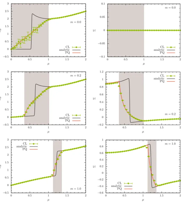
Figure 5. µ-scan for m= 0 (upper panels), m= 0.2 (middle panels) and m= 1 (lower panels) for the random matrix model (2.2) with matrix size N = 48. The shaded region corresponds to that outlined in figure 1. Again we show the baryon number density on the left and the chiral condensate on the right.

JHEP03(2018)015

where we have simplified the notation by introducing the matrix G,

G = (m

− µ

+ Y X − iµ(X + Y ))

. (3.6) The first step in our simulations is to establish that in the absence of a baryon chemical potential, when the action is real, the real Langevin simulations give the correct analytical answer. This is shown in figure 2 where the baryon number (left) and the chiral condensate (right) are plotted as a function of the mass m. We also check the N dependence of our results to confirm that the results are independent of the matrix size. This is also important when comparing our results to those from the phase quenched analytic results, as these are computed in the large N limit. Figure 3 shows the baryon number (left) and the chiral condensate (right) at two different matrix sizes, and we conclude that N = 48 is sufficient.

Finally, we show that our results do not depend on the step size of the discretized Langevin equation. As is demonstrated in figure 4 for the baryon number (left) and the chiral condensate (right), a choice of ∆t = 10

is sufficient to eliminate discretization errors.

Having convinced ourselves that the CL algorithm has been implemented correctly we now simulate the random matrix model at nonzero chemical potential and compare the numerical data to the analytical results, as well as the corresponding large N phase quenched ones. In figure 5 we show the baryon density (left) and the chiral condensate (right) as a function of µ for m = 0 (upper row), m = 0.2 (middle row) and m = 1 (bottom row). Quite surprisingly, we find that our numerical CL results agree with the analytical phase quenched results, and only see agreement with the dynamical one flavor results when these coincide with the phase quenched results. This is the case when the quark mass is outside the domain of the eigenvalues of the Dirac operator, or equivalently, when the chemical potential is outside the domain of the eigenvalues of γ

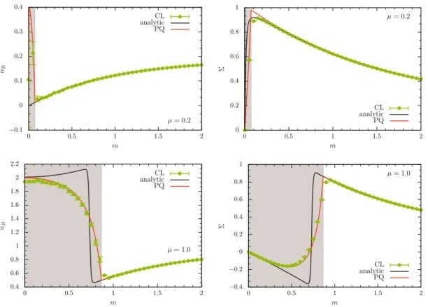
D. In figure 6 we show the baryon density and the chiral condensate as a function of the quark mass for µ = 0.2 (top row) and µ = 1 (bottom row), from which we draw similar conclusions. The shaded regions in figures 5 and 6 and further down in the paper denote the region where the quark mass is inside the domain of the Dirac spectrum (shaded region in figure 1).

We thus conclude that the CL algorithm fails in the region when the baryon number density and the chiral condensate are not holomorphic functions of the matrix elements. We will discuss this in more detail in the next section where we discuss the fermion determinant and the Dirac spectrum.

4 The Dirac spectrum and the fermion determinant

One of the requirements for the correct convergence of CL is that the “operator”, in our case

Tr 1

D + m and Trγ

1

D + m , (4.1)

is a holomorphic function of the complexified variables. This is not the case for the chiral

condensate when the quark mass is inside the two-dimensional locus of the eigenvalues of

D, or equivalently, for the baryon density if the chemical potential is inside the spectral

support of γ

D, which is also a two-dimensional domain. So for the CL to be convergent we

JHEP03(2018)015

−0.1 0 0.1 0.2 0.3 0.4

0 0.5 1 1.5 2

µ= 0.2 nB

m

analyticCL PQ

0 0.2 0.4 0.6 0.8 1

0 0.5 1 1.5 2

Σ

m

analyticCL PQ

µ= 0.2

0.4 0.6 0.8 1 1.2 1.4 1.6 1.8 2 2.2

0 0.5 1 1.5 2

nB

m

analyticCL PQ

µ= 1.0

−0.4

−0.2 0 0.2 0.4 0.6 0.8 1

0 0.5 1 1.5 2

Σ

m

analyticCL PQ

µ= 1.0

Figure 6. Mass scan for µ= 0.2 (upper panels) andµ= 1 (lower panels) for the random matrix theory (2.2) with matrix sizeN= 48. In both cases we plot the baryon number density on the left and the chiral condensate on the right.

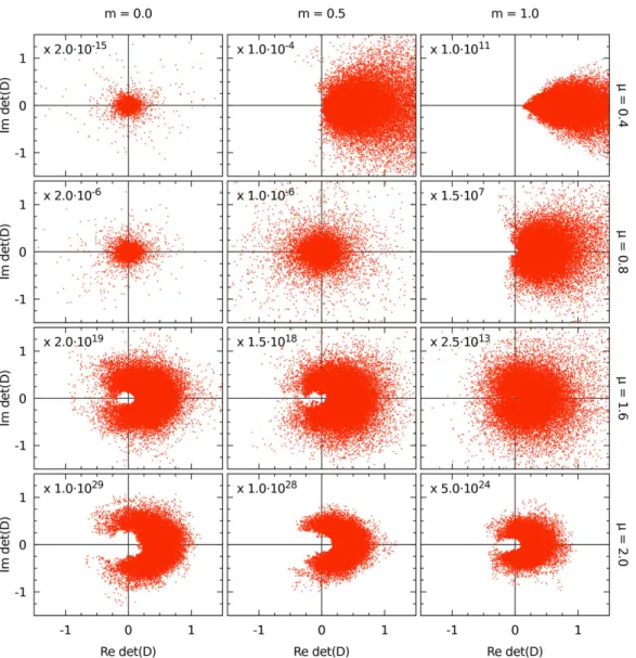
need to require that det(D+µγ

+m) = det(γ

(D +m)+µ) > ε with ε a finite constant. In figure 7 we show scatter plots of the determinant in the complex plane, obtained during the CL simulation for zero and nonzero mass, respectively. Indeed, we will find that simulations converge well when the flow of the determinant avoids the origin, as has also been observed, for example, for the Osborn RMT model [36] and for two-dimensional QCD [41].

In random matrix theory the effect of the fermion determinant on the global distri-

bution of the eigenvalues is a 1/N -correction, and will re-arrange only a small number

of eigenvalues near zero. Also for a nonzero imaginary chemical potential the quenched

and the dynamical eigenvalue distribution are the same for large N . For real chemical

potential the eigenvalue distribution is complex because of the phase of the fermion deter-

minant, but for large N the spectral support is still the same as for the quenched or phase

quenched theory. Since a fermion determinant does not change the overall spectral density

to leading order in 1/N , we expect that also for real chemical potential the distribution of

the eigenvalues will not be affected significantly by the CL evolution. Indeed, as can be

seen in figure 8, where we plot the eigenvalues of the Dirac operator, for various values of

the chemical potential, the support of the Dirac eigenvalues on the CL trajectory is still

given by the quenched result (green curve). Since the CL algorithm is probabilistic we thus

necessarily have that the chiral condensate and the baryon number, which are determined

JHEP03(2018)015

Figure 7. Scatter plots of the fermion determinant of the random matrix model (2.2) with matrix sizeN = 48 for quark massesm={0.0,0.5,1.0}, and chemical potentialsµ={0.4,0.8,1.6,2.0}.

by the distribution of Dirac eigenvalues, will be given by the (phase-)quenched result, as we have seen in figures 5 and 6. In the next section we will show that the correct result can be obtained using a reweighting algorithm.

5 Reweighted complex Langevin

After having established that the CL algorithm fails to reproduce the known analytical

results of the random matrix model (2.2), the obvious question to be asked is if something

can be done to fix the pathologies of the algorithm in regions of the parameter space where

it fails. We apply the reweighted complex Langevin (RCL) method [42–44], and we will

show that one can significantly improve the convergence properties of the algorithm. This

will lead to correct results for values of the parameters for which a naive implementation

JHEP03(2018)015

Figure 8. The Dirac spectrum of the random matrix model (2.2) with matrix size N = 48, for twenty configurations, form= 0 and µ={0.2,0.8,1.0,1.2}.

of the CL algorithm was giving wrong results. Our efforts to test the algorithm will be focused on the region close to the phase transition.

The motivation of the method mainly comes from the expectation that reweighting CL trajectories might work better than other traditional forms of reweighting, mainly because the target ensemble with parameters (ξ = m, µ) and the auxiliary ensemble with parameters (ξ

= m

, µ

) are expected to have larger overlap. In reweighting one computes the expectation value of an observable O using

hOi

=

R dx w(x; ξ) O (x; ξ) R dx w(x; ξ) =

R dx w(x; ξ

) h

w(x;ξ)

w(x;ξ0)

O (x; ξ) i R dx w(x; ξ

) h

w(x;ξ) w(x;ξ0)

i =

D

w(x;ξ0)

O (x; ξ) E

ξ0

D

E

ξ0

. (5.1)

However, contrary to the traditional forms of reweighting, the weight w(x; ξ

) = e

is complex, and thus, we need to employ the CL algorithm to sample this auxiliary ensemble.

Of course, this is performed through a judicious selection of the reweighting parameters, chosen from the region where the algorithm satisfies the CL convergence properties. In this case the reweighting equation becomes, after complexification of the variables,

hOi

=

R dxdy P (z; ξ

) h

w(z;ξ)

w(z;ξ0)

O (z; ξ) i R dxdy P (z; ξ

) h

w(z;ξ) w(z;ξ0)

i , (5.2)

JHEP03(2018)015

0.5 1 1.5 2 2.5

0 0.5 1 1.5 2

nB

m

RCLCL analytic

µ= 1.0

−0.4

−0.2 0 0.2 0.4 0.6 0.8 1

0 0.5 1 1.5 2

Σ

m

RCLCL analytic µ= 1.0

0 0.5 1 1.5 2 2.5

0 0.5 1 1.5 2

nB

µ

RCLCL analytic m= 0.2

−0.2

−0.1 0 0.1 0.2 0.3 0.4 0.5 0.6 0.7 0.8 0.9

0 0.5 1 1.5 2

Σ

µ

RCLCL analytic

m= 0.2

Figure 9. Results for the RCL method for the random matrix model (2.2) with matrix sizeN = 6.

The mass scan for µ= 1 (upper panels) is generated from an auxiliary ensemble with m0 = 4 at the same µ, while theµ-scan for m= 0.2 (lower panels) uses an auxiliary ensemble atµ0= 2 and same mass. We show the baryon number density on the left and the chiral condensate on the right.

where P (z; ξ

) is the real probability in the complex variables z = x + iy, generated by the CL trajectory. In practice, the configurations of the auxiliary ensemble are sampled according to their probability P (z, ξ

) in the complexified variables by evolving the CL equations for the auxiliary action. An expectation value in the target ensemble is then computed as a ratio of the average effective observable and the average reweighting factor, both measured along the auxiliary CL trajectories.

We first test the method with small matrices (N = 6) and we see in figure 9 that reweighting the CL trajectories can fix all the problematic issues of the algorithm. It is interesting to observe that for this relatively small matrix size the analytical answer can be reproduced for the whole range of parameters, as can be seen from the scans of the mass and of the chemical potential. It is important to stress that this is already quite intriguing since the naive implementation of the algorithm was failing to reproduce the correct answer in the region where the operators are non-holomorphic. Moreover, it is interesting to observe that, even though the auxiliary ensemble is chosen at one side of the phase transition, i.e., with large m

for the mass scan or large µ

for the µ-scan, the RCL data at the other side of the phase transition still agree very well with the analytical results.

Nevertheless, we already notice that the error bars start to grow in the phase transition

region, as is expected if the sign problem grows in that region.

JHEP03(2018)015

0.5 1 1.5 2 2.5

0 0.2 0.4 0.6 0.8 1 1.2

nB

m

RCLCL analytic

µ= 1.0 _−0.4

−0.2 0 0.2 0.4 0.6 0.8 1

0 0.2 0.4 0.6 0.8 1 1.2

Σ

m

RCLCL analytic µ= 1.0

0 0.5 1 1.5 2 2.5

0 0.2 0.4 0.6 0.8 1 1.2 1.4

nB

µ

RCLCL analytic m= 0.2

−0.4

−0.2 0 0.2 0.4 0.6 0.8 1 1.2

0 0.2 0.4 0.6 0.8 1 1.2 1.4

Σ

µ

RCLCL analytic

m= 0.2

Figure 10. Results for the RCL method for to the random matrix model (2.2) with matrix size N = 24. The mass scan for µ = 1 (upper panels) is generated from an auxiliary ensemble with m0 = 1.3 and sameµ, while the µ-scan for m= 0.2 (lower panels) uses an auxiliary ensemble at µ0 = 1.5 and same mass. Again we show the baryon number density on the left and the chiral condensate on the right.

Of course in order to claim to have solved the sign problem, which is exponentially hard

with respect to the volume of the system, we need to show that the number of matrices

needed to achieve the sought precision does not scale exponentially with the matrix size

N . For this reason we increased the matrix size, in order to investigate if this method

of reweighting actually works and how it scales with respect to the matrix size N . In

figure 10 we show the RCL data for N = 24. The upper graphs show a mass scan for

fixed µ and the lower graphs a µ scan for fixed mass. To keep the error under control in

the phase transition region the number of configurations had to be increased by a factor

of 100 compared to N = 6. This allows us to have small error bars in the mass scan for

µ = 1.0, for all mass values. In this scan the RCL always gives the correct value even

though CL obviously fails as soon as m < 1.0. In the µ-scan we see that RCL is able to

improve on the CL method outside the phase transition, however, inside this region, i.e.,

for 0.6 < µ < 0.8, the sign problem clearly reappears. The figure plainly shows that RCL

performs qualitatively better than the CL method in all cases, but with the caveat that the

phase transition region is still difficult to access. Undoubtedly, the same is true for N = 48

as can be seen in figure 11. The RCL works reasonably well in the mass scan, performed

for µ = 1, whereas the CL does poorly over most of the mass range. Unfortunately, the µ

JHEP03(2018)015

0.5 1 1.5 2 2.5

0 0.2 0.4 0.6 0.8 1 1.2

nB

m

RCLCL analytic

µ= 1.0 _−0.4

−0.2 0 0.2 0.4 0.6 0.8 1

0 0.2 0.4 0.6 0.8 1 1.2

Σ

m

RCLCL analytic µ= 1.0

0 0.5 1 1.5 2 2.5

0 0.2 0.4 0.6 0.8 1 1.2 1.4

nB

µ

RCLCL analytic m= 0.2

−0.4

−0.2 0 0.2 0.4 0.6 0.8 1 1.2

0 0.2 0.4 0.6 0.8 1 1.2 1.4

Σ

µ

RCLCL analytic

m= 0.2

Figure 11. Results for the RCL method for the random matrix model (2.1) with N = 48. The mass scan forµ= 1 (upper panels) is generated from an auxiliary ensemble withm0= 1.3 and same µ, while the µ-scan form = 0.2 (lower panels) uses an auxiliary ensemble at µ0 = 1.5 and same mass. Again we show the baryon number density on the left and the chiral condensate on the right.

scan distinctly shows that the reweighting only works above and below the phase transition region. Again we observe the salient feature that even though the auxiliary ensemble is taken at one side of the phase transition, the reweighting procedure reproduces the data well also at the other side of the transition. This seems to point to the absence of an overlap problem in the RCL method, even though the sign problem is clearly present in the phase transition region. One disturbing point of this investigation is that it confirms how bad the original CL performs for a very large range of parameters, even away from the phase transition. Indeed, the CL seems to fail in regions where reweighting still works quite well and is not yet hampered by the sign problem.

Using the data for N = 6, 12, 24, 48 we find a naive volume scaling for the RCL method that is proportional to exp(0.3 × N ) for the number of configurations necessary to get the same accuracy for all values of N . This shows that, even though this reweighting method rectifies the failing of the CL method for a large range of parameter values, it still is exponential in the volume in the phase transition region.

6 Shifted representation

In an attempt to mend the problems due to the phase of the Dirac operator we now shift

the effect of the chemical potential away from the fermionic term. This can be done with a

JHEP03(2018)015

-0.15 -0.1 -0.05 0 0.05 0.1 0.15 0.2 0.25 0.3

✵ ✺✁✂✄ ☎

✹

✶✆✝ ✞✟✠

✡

☛☞✌ ✍✎✏

✑

✷ ✒✓✔✕ ✖

✗

tr(Are) / N

steps

standard shifted

0 0.005 0.01 0.015 0.02 0.025 0.03 0.035 0.04

✵ ✺✁✂✄ ☎

✹

✶ ✆✝✞✟ ✠

✡

☛ ☞✌✍✎ ✏

✑

✷ ✒✓✔✕ ✖

✗

tr(Aim) / N - (µ)shifted

steps

standard shifted

✲✘✙ ✚

✛✜✢ ✣

✥

✤✦✧

★✩✪

✫✬✭

✮✯✰

✱✳✴

✸ ✻✼✽ ✾ ✿❀ ❁❂❃❄ ❅❆❇❈❉❊❋ ●❍■❏❑▲▼◆ ❖P◗❘❙❚❯❱❲ ❳❨

steps

st❩❬❭❪ ❫❴

❵❛❜❝ ❞❡❢

❣❤✐ ❥

❦❧♠ ♥

♦

♣qr

✉✈✇

①②③

④⑤⑥

⑦⑧⑨

⑩ ❶❷❸ ❹ ❺❻ ❼❽❾❿ ➀➁➂➃➄➅➆ ➇➈➉➊➋➌➍➎ ➏➐➑➒➓➔→➣↔ ↕➙

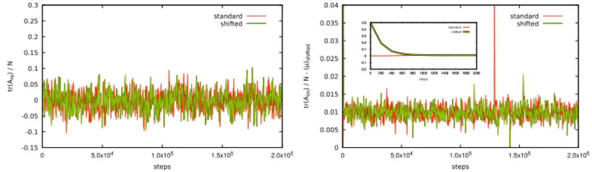
Figure 12. Complex Langevin evolution of the real (left) and imaginary (right) parts of the average diagonal entry of A and A⁰ in the standard and shifted representation of the random matrix theory (2.2), respectively. The shiftedA⁰ is subtracted byiµ.

simple shift of variables. Written out in the Cartesian representation, the Dirac operator is

D = m iA − B + µ

iA

+ B

+ µ m

!

. (6.1)

We can absorb µ into A with a simple change of variables, A

= A − iµ. The action in terms of the matrices A

and B is

S = N tr A

A

+ 2iµA

− µ

+ B

B

− N

tr log m

+ X

Y

, (6.2)

where X

= A

+iB and Y

= A

− iB

. In this representation the µ dependence has been shifted from the fermionic to the bosonic term. Computing the CL force term results in

∂S

∂A

= 2N (A

+ iµδ

) − N

X

G

+ (G

Y

)

mn

, (6.3a)

∂S

∂B

= 2N B

+ iN

X

G

− (G

Y

)

mn

, (6.3b)

where G

= (m

+ Y

X

)

is defined in terms of the shifted fields. The advantage of the shifted representation is that it starts in an anti-Hermitian state, and due to the fact that CL is non-deterministic, the configurations could potentially evolve to a different minimum.

To analyze the dynamics of the shifted representation we analyze the elements of the matrices A and A

during CL evolution; the real and imaginary part of their average diagonal entry are shown in figure 12. Although the two matrices start out very differently, they are similar after thermalization. This seems to indicate that

A

CL,shifted

= A

CL,standard

− iµ, (6.4)

and thus they converge to the same solution. Since the Dirac operator in the shifted

representation starts the CL evolution at a chiral condensate and a baryon number density

for µ = 0, one might expect better convergence properties at least below the critical value

of the chemical potential. In the next section we will use the shifted representation when

analyzing the effect of gauge cooling.

JHEP03(2018)015

7 Gauge cooling

The complexified action takes on redundant degrees of freedom which is evident from the fact that the action is invariant under an enhanced symmetry group as compared to the original RMT. One can utilize this enlarged symmetry in an attempt to steer the Langevin flow towards more physical configurations due to the fact that although the action is invariant under these transformations, the flow itself is not. This method is commonly referred to as gauge cooling, and has been used to great effect in a plethora of models [14, 45]. Most relevant to our study is its successful application to the Osborn RMT model (2.6) [45], which we will refer to for comparison.

The original RMT is invariant under the U(N ) transformation

W → gW g

, W

→ gW

g

where g ∈ U(N ). (7.1) However the complexified action is invariant under the enlarged GL(N, C ) transformation X → hXh

, Y → hY h

where h ∈ GL(N, C ). (7.2) We stress that the cooling transformation does not change the eigenvalues of the Dirac operators D and γ

(D + m), and that the effect of cooling occurs in tandem with the Langevin updates. Next we will look at how to choose h in an advantageous way.

7.1 Cooling norms

The transformation matrices h are chosen such that a cooling norm is reduced. These norms are constructed to quantify an undesirable property of the matrix configurations.

The most basic of these is the Hermiticity norm [45]

N

= 1 N tr h

X − Y

X − Y

i

, (7.3)

which measures the deviation of the CL configuration from a valid RMT configuration. It is zero when X

= Y , and grows when the matrices A and B acquire imaginary parts.

We also introduce an eigenvalue norm [45]

N

=

nev

X

i=1

e

(7.4)

where γ

are the n

lowest eigenvalues of the positive definite matrix D

D, and ξ is a real positive parameter. This norm suppresses configurations with Dirac eigenvalues close to zero.

Finally, we will also use a generalization of the anti-Hermiticity norm, N

= 1

N tr h

ϕ + ψ

ϕ + ψ

i

, (7.5)

which was introduced in [45] for p = 1. The matrices ψ and ϕ are the off-diagonal elements of D. For the Stephanov model they are given by ψ = iX + µ and ϕ = iY + µ, so that the norm becomes

N

= 1 N tr h

iX − iY

+ 2µ

iY − iX

+ 2µ

i

. (7.6)

JHEP03(2018)015

For p = 1 the µ-dependent terms do not depend on the similarity transformation h, and the Dirac operator is generally not anti-Hermitian at the minimum of the norm. Therefore will use the p = 2 anti-Hermiticity norm below.

As the different norms try to fix different problems one can also combine them in ag- gregate norms. One useful choice is to combine the Hermiticity norm, which quantifies how much the configurations drift into the imaginary plane, with either the anti-Hermiticity or the eigenvalue norm, both of which handle problematic configurations related to a singular behavior of the drift

N

= (1 − s)N

+ sN

, where s ∈ [0, 1]. (7.7) 7.2 Computing h

We follow the procedure outlined in [45] to compute the transformation matrix h. We can write h in terms of the U(N ) generators, λ

∈ u(N )

h = e

, a

∈ C . (7.8)

Because the RMT is invariant under U(N ) transformations, we can choose a

∈ R to only pick out the GL(N, C )/U(N ) transformations. Assuming the norm is a function N (X, Y ) we want to solve the following equation

h ˜ = n e

a

= arg min

a⁰_i

N e

Xe

, e

Y e

o

. (7.9)

This can be reduced to a one dimensional minimization problem by first computing the gradient descent vector of the transformation through

˜

a

= − ∂

∂a

N

, (7.10)

and then solve the one parameter minimization problem

˜ h ≈ n e

β = arg min

β⁰

N e

Xe

, e

Y e

o

. (7.11)

where β is a real positive quantity. β is computed by applying Brent’s method [46], to which we add an upper bound to avoid a numerically unstable minimization. We take this upper bound to be 0.1. The derivative of the norm with respect to a

can be computed either numerically or analytically depending on the norm. After applying the similarity transformation X → hXh

and Y → hY h

, the derivative of the Hermiticity norm is

∂

∂a

N

= 2

N tr Y

[λ

, Y ] + X

[λ

, X]

, (7.12)

where [A, B] is the standard commutator. After applying the similarity transformation to ϕ and ψ in (7.5), the derivative of the p = 2 anti-Hermiticity norm is found to be

∂

∂a

N

= 2 N tr

(ϕ

+ ψ)(ϕ + ψ

) ϕ

[λ

, ϕ] − ϕ

[λ

, ψ

] + ψ[λ

, ϕ] − ψ[λ

, ψ

]

− [λ

, ϕ

]ϕ − [λ

, ϕ

]ψ

+ [λ

, ψ]ϕ + [λ

, ψ]ψ

. (7.13)

Finally, the derivative of the eigenvalue norm is computed numerically.