A modular framework for simulations of Ionization Profile Monitors – Implementation
and Benchmarking
Dominik Vilsmeier June 15, 2017
Supervisors:
Prof. Dr. Tilo Wettig (Universit¨at Regensburg)
Dr. Mariusz Sapinski (GSI Helmholtz Centre for Heavy Ion Research)
Abstract
Simulations of electron and ion tracking in Ionization Profile Monitors are an important tool for specifying and designing new monitors. They are also essential for understanding the effects related to the ionization process, guiding field non-uniformities and influence of the beam fields which may lead to a distortion of measured beam profiles. Most of these effects cannot be treated analytically and therefore several simulation codes have been developed at different accelerator laboratories during the past years. Those existing codes are often tuned to the specific needs of a laboratory, are not well documented and lack a practical user interface. This work presents a novel, generic simulation tool with focus on the ability to test, maintain and extend the code. A complete documentation as well as facile usage were important aspects too. The application combines the features of existing codes in order to provide a common standard for IPM simulations. Because of its modular structure the application allows for exchanging the computational modules depending on the use case as well as for straightforward extensibility to new use cases. Future intended use cases are for example simulations of Beam Induced Fluorescence monitors based on gas jets or Electron Wire Scanners. The current set of algorithms includes several particle tracking methods (for instance Runge-Kutta 4th order or the Boris algorithm) and several bunch field evaluation algorithms (analytical solutions for specific cases as well as numerical Poisson solvers). The application and all involved methods have been tested and benchmarked against existing results. The code is well documented and includes a graphical user interface. It is publicly available as a git repository and as a Python package.
1. Introduction 6
2. Requirements & Use cases 8
2.1. Use cases . . . 8
2.1.1. Profile deformation due to beam space charge . . . 8
2.1.2. Profile deformation due to guiding field non-uniformities. . . 8
2.1.3. Simulation of meta-stable excited states and their influence on the measured beam profile (BIF) . . . 9
2.1.4. Gas jets for IPM and BIF . . . 9
2.1.5. Electron background . . . 9
2.1.6. Secondary electrons . . . 10
2.1.7. Electron Wire Scanner . . . 10
2.1.8. Correlations between electron and ion detection. . . 10
2.1.9. Simulating multiple beams . . . 10
2.1.10. Studying trajectories of specific particles. . . 11
2.2. Requirements . . . 11
3. Components 13 3.1. Model & Manager . . . 13
3.2. Particle generation . . . 13
3.2.1. Ionization . . . 16
3.3. Particle tracking . . . 17
3.4. Devices . . . 17
3.5. Guiding fields . . . 18
3.6. Beams . . . 19
3.6.1. Bunch trains . . . 19
3.6.2. Bunch shapes . . . 20
3.7. Beam fields . . . 21
3.7.1. Bunch electric field models . . . 22
3.8. Output recorders . . . 23
3.9. Auxiliaries . . . 23
3.9.1. Simulation cycle . . . 23
3.9.2. Particle Supervisor . . . 24
3.9.3. Setup . . . 24
3.10. Configuration . . . 25
3.11. Start & Setup . . . 27
4. Available models 29 4.1. Particle Generation . . . 30
4.1.1. Single particle generation . . . 30
4.1.2. Manual generation of particles . . . 30
4.1.3. Ionize particles at a fixed z-position . . . 30
4.1.4. Ionization cross sections . . . 30
4.1.5. Electron gun (pending) . . . 32
4.1.6. Secondary electrons (pending) . . . 34
4.1.7. Gas jet (pending). . . 34
4.2. Particle tracking . . . 34
4.2.1. Runge-Kutta 4th order . . . 34
4.2.2. Boris algorithm . . . 36
4.2.3. Analytical solutions . . . 36
4.3. Devices . . . 37
4.3.1. Ionization Profile Monitor . . . 37
4.3.2. Beam Induced Fluorescence monitor (pending) . . . 37
Contents
4.4. Guiding fields . . . 38
4.4.1. Uniform fields. . . 38
4.4.2. Field maps . . . 38
4.5. Bunch electric field models . . . 38
4.5.1. Symmetric Gaussian (analytical, 2D) . . . 38
4.5.2. Asymmetric Gaussian (analytical, 2D) . . . 39
4.5.3. Parabolic ellipsoid (analytical, 3D) . . . 40
4.5.4. Poisson solver based on Successive Over-Relaxation (numerical, 2D) . 40 4.5.5. Poisson solver based on Finite Elements (numerical, 3D) . . . 41
4.6. Output recorders . . . 42
4.6.1. Mapping of initial to final particle attributes . . . 42
4.6.2. Studying trajectories . . . 42
4.6.3. Beam profiles in XML format . . . 42
5. Benchmarking 43 5.1. Particle tracking . . . 43
5.1.1. Gyro motion . . . 43
5.1.2. E×B-drift . . . 44
5.1.3. Trajectories with beam fields . . . 46
5.2. Bunch electric field models . . . 48
5.2.1. LHC case . . . 48
5.2.2. PS case . . . 51
5.3. Profile comparison . . . 51
5.3.1. LHC case . . . 52
5.3.2. PS case . . . 52
5.3.3. SIS-18 measurements. . . 53
5.4. Performance. . . 56
5.4.1. Particle tracking . . . 56
5.4.2. Bunch electric field models . . . 57
6. Summary and Conclusions 59 References 61 Appendices 64 A. How to install the application 64 A.1. Installation . . . 64
A.1.1. Via Anaconda (recommended) . . . 64
A.1.2. Manual installation (advanced) . . . 65
A.1.3. Verifying the installation . . . 67
A.1.4. Creating a desktop entry . . . 67
A.2. Updating the package . . . 67
A.2.1. For installations via Anaconda . . . 67
A.2.2. For manual installations . . . 67
A.3. Uninstalling the package . . . 68
B. How to use the application 68 B.1. Conventions . . . 68
B.2. Via the command line . . . 68
B.3. Via the GUI. . . 69
B.3.1. Configuration . . . 69
B.3.2. Simulation . . . 71
B.3.3. How can I test the current configuration? . . . 72
B.4. Output . . . 72
B.4.1. How can I check the output? . . . 72
B.5. Command line tools . . . 73
1. IPM sketch . . . 6
2. Package structure. . . 14
3. Cross-dependency diagram. . . 15
4. Iteration flowchart . . . 15
5. Particle generation sub-package structure . . . 16
6. Particle tracking sub-package structure. . . 18
7. Devices sub-package structure . . . 18
8. Beams sub-package structure . . . 19
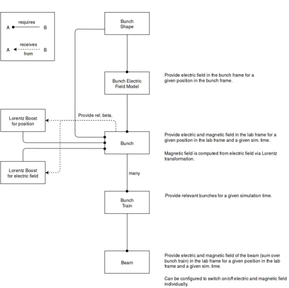
9. Beam field acquisition diagram . . . 22
10. Configuration diagram . . . 27
11. Simulation flowchart . . . 28
12. Model overview . . . 29
13. Sketch of generating all particles at a fixed z-position. . . 31
14. Double differential cross section . . . 32
15. Single differential cross sections with respect to energy . . . 33
16. Single differential cross sections with respect to the scattering angle . . . 33
17. Momentum shift for the Boris algorithm . . . 37
18. Results for the gyro motion and the E×B-drift test cases . . . 45
19. Energy- and y-deviation for the gyro motion test case . . . 45
20. Trajectories for the E×B-drift test case . . . 46
21. Trajectories for the LHC case . . . 47
22. Electric field estimation for large field gradients . . . 48
23. Trajectories for the 3 kV PS case . . . 49
24. Trajectories for the 3 kV PS case with magnetic field . . . 49
25. Bunch electric field (LHC case) . . . 50
26. Charge density (LHC case) . . . 51
27. Longitudinal electric field from the Parabolic Ellipsoid model (LHC case) . . 51
28. Bunch electric field (PS case) . . . 52
29. Charge density (PS case) . . . 52
30. Profile comparison (LHC case) . . . 53
31. Profile comparison (PS cases) . . . 53
32. Mapping of initial vs. final x-positions (PS cases) . . . 54
33. SIS-18 vertical measurement, 8 kV extraction voltage, image . . . 55
34. SIS-18 vertical measurement, 8 kV extraction voltage, profiles . . . 55
35. Initial momenta for the SIS-18 simulations. . . 55
36. SIS-18 horizontal measurement, 8 kV extraction voltage, image . . . 56
37. SIS-18 horizontal measurement, 8 kV extraction voltage, profiles . . . 57
38. Particle tracking performance . . . 57
39. Bunch electric field models performance . . . 58
40. Screenshot of the configuration GUI . . . 70
41. Screenshot of the simulation GUI . . . 71
42. Screenshot of the post-analysis GUI . . . 73
1. Introduction
Ionization Profile Monitors (IPM) are used for measuring the transverse profile of particle beams. Those devices make use of the rest gas ionization by the particle beam and guide the ionization products (ions and/or electrons) towards a detector with the help of an external electric field. Figure1shows a sketch of an IPM. The main electrodes at the top and bottom and the side electrodes together form the high voltage cage (HV cage). The side electrodes are commonly used for increasing the uniformity of the electric guiding field however designs without side electrodes that have a good field uniformity exist as well [1]. Various acquisition systems are available, figure 1 illustrates the usage of a multi-channel plate (MCP) for amplifying the incoming electron signal, followed by a phosphor screen for converting the electron signal into an optical signal. The produced light is guided by a prism to a camera which records the resulting distribution. The recorded image is a projection of the transverse beam profile for a particular transverse direction. Other possible acquisition systems include arrays of metal strips for detecting the electron signal or pixel detectors which allow for registering a much smaller electron signal [1].
However there are many effects that can influence the quality of measured profiles and thus can make the design and operation of IPMs difficult. Among the effects that directly influence the quality of the measured electron signal the most important ones to mention are [3,4]:
• Initial velocities obtained during the ionization process: Electrons may obtain a sub- stantial kinetic energy during the ionization process and therefore do not move on straight lines towards the detector. Any transverse velocity component introduces a displacement of the measured electrons and therefore a distortion of the measured profiles may become visible.
• Guiding field non-uniformities: A uniform guiding field in the relevant detector region is important to ensure that all electrons are likewise guided towards the detector. However
Figure 1: Sketch of an Ionization Profile Monitor [2, H. Refsum] with an optical acquisition system including a phosphor screen, a prism and a camera. A multi-channel plate is used for amplifying the electron signal.
1. Introduction
because of the finite size of the electrodes field non-uniformities at the boundaries might play a role and result in a profile distortion.
• Beam space charge interaction: The ionization products interact with the electromag- netic field of the particle beam and depending on the beam parameters this interaction can get so strong that the trajectories of particles are significantly distorted resulting in a distortion of the overall profile.
Some of the effects can be compensated by applying an additional magnetic guiding field which is aligned with the electric guiding field. Electrons then spiral around the magnetic field lines and the extent of this gyro motion limits their maximum displacement. However for large beam energies and small beam sizes this compensation might not be sufficient to suppress possible distortions [3].
Because the treatment of those effects is rather complicated and cannot be done analytically it is essential to study them by means of simulations. This is helpful not only for obtaining a deeper understanding of the profile distortions but also for designing devices by verifying that one can expect a good signal quality from a particular set of specifications. For those reasons several simulation codes have been developed at different particle accelerator laboratories during the past years [5–11]. Much interest in further development of IPM simulations has been shown at a dedicated workshop held at the European Center for Nuclear Research (CERN) in 2016 (https://indico.cern.ch/event/491615/) and was reconfirmed at a follow-up workshop held at the GSI Helmholtz Center for Heavy Ion Research (GSI) in 2017 (https://indico.gsi.de/event/IPM17/).
The existing codes are often tuned to the specific needs of the laboratory they have been developed at. Often they are not well documented and do not include a practical user interface which makes it difficult to use or reuse parts of them. The codes often consist of short scripts for Matlab for example and thus the procedures are not easily reusable in other projects. For those reasons the idea of establishing a common simulation tool which combines the features of the existing codes into a single application was born. Such an application should be well documented, tested and benchmarked against existing results as well as measurement data in order to prove the integrity of the implemented methods and to highlight their applicability for different use cases. A clear and modular code structure is highly desirable in order to ensure testability of the single components as well as extensibility to new components and new use cases. The maintainability of the code will also largely benefit from a modular code structure. A graphical user interface is desired in order to facilitate configuring and running simulations as well as to provide simple post-processing tools that allow for quick analyses of the simulated results. Because simulations of other devices such as Beam Induced Fluorescence monitors (BIF) or Electron Wire Scanners involve similar procedures as IPM simulations (most importantly the movement of charged particles in the electromagnetic field of a particle beam along with dedicated methods for generating and detecting those particles) they are foreseen as future use cases as well and thus the design of the application should bear them in mind.
2. Requirements & Use cases
2.1. Use cases
In order to fix the requirements of the application various use cases are discussed below.
Defining a clear set of requirements helps to maintain consistency during the development process and avoids unnecessary rework of components or the whole framework. All use cases refer to beam profile monitors which involve the interaction of measured particles with the electromagnetic field of the particle beam and therefore potentially suffer from a displacement which can result in a distortion of the measured profiles.
2.1.1. Profile deformation due to beam space charge
Ionization Profile Monitors make use of the rest gas ionization by the particle beam. By guiding the ionization products towards a detector (multi-channel plate and phosphor screen or pixel detector for example) with the help of an external electric (and magnetic) field one can obtain a projection of the beam’s charge distribution for a specific transverse plane.
If the beam current is sufficiently high or the beam is sufficiently small then deformation effects due to the interaction of ions or electrons with the beam space charge start to play a role [3,4]. Instead of traveling on straight lines towards the detector the ionization products suffer from displacements with respect to their initial positions, leading to a deformation of the measured profile. This scenario involves simulating the movement of charged particles (ions or electrons) in the presence of external guiding fields as well as the electromagnetic field of the particle beam. The initial distribution of electrons arises from the interaction of the beam with the rest gas due to ionization. The initial momenta are also obtained during the ionization process. The particles are tracked towards a detector where their final positions and/or momenta are recorded and form the measured profile.
2.1.2. Profile deformation due to guiding field non-uniformities
Guiding field non-uniformities depending on the design of the high voltage cage (HV cage) or the placement of electrodes can have a significant impact on the trajectories of ions or electrons. Those non-uniformities might occur as unwanted by-products in form of fringe fields at the longitudinal boundaries of the HV cage or they might represent a feature of the monitor as described in [12]. With regard to ionization it is important to accurately represent the ionization process in the complete relevant volume of the monitor (which is governed by a pressure bump for example). In addition this scenario involves similar aspects as the profile deformation due to beam space charge (see section2.1.1).
2.1. Use cases
2.1.3. Simulation of meta-stable excited states and their influence on the measured beam profile (BIF)
Beam Induced Fluorescence monitors (BIF) make use of the excited states of gas atoms or ions which are induced by the interaction with the particle beam. Those excited states decay under the emission of light and the transverse beam profile can be reconstructed provided that the positions of light emission do not change significantly with respect to the corresponding excitation positions. If the particles travel a certain distance until their excited state decays then this displacement might introduce a distortion of the measured profile [13,14]. This use case aims for investigating the influence of these meta-stable excited states on the displacement of measured particles and therefore on the measured profiles in a BIF monitor. Because the gas atoms are excited by the interaction with the particle beam the distribution of excited atoms follows the distribution of the particles in a bunch.
The further such excited atoms travel during the time until the excited state decays the stronger the measured profile will deviate from the actual beam profile. Thus the decay time is deciding for how long the excited particles will be tracked and how large this effect on the measured beam profile is.
2.1.4. Gas jets for IPM and BIF
In case of ultra high vacuums the number of ionized or excited particles might not be sufficient in order to obtain a stable signal for either Ionization Profile Monitors or Beam Induced Fluorescence monitors (the excitation cross section relevant for BIFs is even smaller than the ionization cross section which is relevant for IPMs). Using supersonic gas jets one can create dedicated regions of high gas density which provide good ionization or excitation rates and therefore generate a good signal for the used detector [14]. The gas motion in supersonic gas jets is substantially different from the rest gas motion where the thermal motion dominates.
Molecules in the gas jet have one dominant velocity component in the direction of the jet (with a very narrow distribution) and relatively small other components. This additional velocity component is inherited by the ionization products (electrons and ions) and might induce a displacement of the measured particles and therefore a distortion of the resulting profiles. In addition density gradients within the gas jet lead to a signal of spatially varying strength and this effect must be accounted for as well. The goal of this use case is to study the effect of gas jet dynamics on the trajectories of ions and electrons which eventually lead to a distortion of the registered profiles. In case of a BIF monitor gas atoms are excited by the interaction with the beam and tracking must be performed until the excited state decays by emission of light.
2.1.5. Electron background
Electrons may emerge not only from the ionization process involving the interaction of the beam with the rest gas in the vacuum chamber but also from various other sources like the onset of electron clouds or radiation fields due to beam losses [15]. Those electrons are
likewise guided towards the detector and registered as a part of the measured profile. The goal is to study the effect of various background electron distributions on the measured profiles. The background electrons hence need to be described by predefined position and velocity distributions.
2.1.6. Secondary electrons
The ion impact on the electrode or on the ion trap grid (which is installed above the electrode and supplied with a slightly larger voltage) causes secondary electron emission. For an IPM working with electron detection those electrons are likewise guided towards the detector and are registered as a part of the measured profile. The goal of this use case is to study the effect of those secondary electrons on the measured profiles. The final position distribution of ions at the ion trap and the geometry of the ion trap itself defines the initial position distribution of secondary electrons. The momenta of impacting ions must be sufficiently large in order to yield secondary electrons. The relevant threshold is material dependent however for typical IPM specifications it is easily exceeded.
2.1.7. Electron Wire Scanner
For an Electron Wire Scanner an electron beam is aligned perpendicular to the particle beam which causes a deflection of the electrons due to its electric (and magnetic) field.
Analyzing the deflection of electrons after they have traversed the beam region one can deduce features of the charge distribution of the beam [16]. A (measured) position and momentum distribution which corresponds to the required electron beam could be provided as an external input resource (emerging from an “electron gun” for example).
2.1.8. Correlations between electron and ion detection
An IPM could detect both electrons and ions emerging from the ionization process with the same beam. Correlations between those measurements allow for conclusions regarding the original beam distribution and could potentially provide deeper insight into the mechanisms of profile distortion. Also one can determine the mode of IPM operation that is suitable for a given beam case.
2.1.9. Simulating multiple beams
Multiple beams (with different particle types) might travel simultaneously through the vacuum chamber as for example in the case of an electron lens or an electron cooler. When measuring the distribution of such beam ensembles the tracked particles are subject to the total electromagnetic field emerging from both beams. Measuring the combined profile of a proton or ion beam which is accompanied by an electron beam (for clearing the beam halo or cooling the proton/ion beam) using a BIF monitor for example the trajectories of excited
2.2. Requirements
ions are influenced by the electromagnetic fields of both beams and will show a different kind of displacement [17]. By using multiple beams one can also emulate the case where consecutive bunches have different parameters as for example for SPS scrubbing runs [18].
2.1.10. Studying trajectories of specific particles
One might want to observe for example only particles which are ionized at the head or the tail of a bunch. Studying trajectories of particles which become trapped inside the bunch (due to the beam field temporarily exceeding the external electric guiding field) is of interest too. By observing the trajectories of single particles one can learn more about the underlying effects that play a role for the displacement of measured particles.
2.2. Requirements
From the above use cases we deduce a set of requirements to which the application shall conform. Those requirements serve as important guidelines during the development process and are chosen such that all discussed use cases can be realized.
1. Each simulation run may involve an arbitrary number of beams (including zero). The combined electromagnetic field of all beams influences the trajectories of tracked particles and therefore the single beam fields cannot be split over multiple runs of the simulation.
2. Each beam consists of one or more identical bunches where two consecutive bunches are separated by an offset greater than zero. Identical means that they have the same shape and parameters, the only difference is their space-time location which leads to different electromagnetic fields measured at a given space-time point in the laboratory frame.
3. Each bunch generates an electric field and is thus assigned a bunch electric field solver.
The electric field is solved in the rest frame of a bunch. The electric and magnetic fields as experienced by the tracked particles are obtained by transforming their four vector positions to the rest frame of a bunch, evaluating the electric field in this reference frame and transforming the result back to the laboratory frame which yields the electric and magnetic field as experienced by the particle (using Lorentz transformations). Two identical bunches share the same electric field solver object.
4. Each simulation involves the tracking of exactly one particle type (electrons or ions of a given type). Use cases which involve multiple particle types to be tracked can be realized by running the simulation multiple times (once per particle type) and then merging the results.
5. The tracked particles are non-relativistic and therefore can be described in a single reference frame (the laboratory frame).
6. Each simulation involves exactly one way of generating particles. Use cases which involve particles being created due to different mechanisms can be realized by running the simulation multiple times (once per mechanism) and then merging the results.
7. Each simulation involves exactly one electric guiding field specifier and one magnetic guiding field specifier.
8. The external electric and magnetic guiding fields may vary in time.
9. Each particle is in a defined state at every time during the simulation. Different states are possible, such as “tracked”, “detected” or “invalid”. A particle’s state may be changed by the components of the application.
10. Each simulation takes place in the environment of exactly one “device” which defines the boundaries of the simulation as well as modifies the particles’ statuses by deciding when particles are considered to be detected or invalid.
11. The (type of) output of a simulation is configurable however only involves data from the tracked particles. Other data (such as beam field maps for example) shall be generated by other means which are not part of the actual simulation (dedicated scripts can be used for such tasks).
12. The components of the application might depend on each other (for example the particle tracking needs information about the electromagnetic fields). Therefore each component may declare a number of other components as dependencies in order to use attributes or functionality from them.
13. Each component may declare a number of parameters which provide a way of configuring this component through an external configuration source. For each simulation the user must supply such a configuration source which covers all parameters that have been declared by the involved components.
14. The user may specify which particular solution they want to apply to the different part problems of the simulation. For example a user may specify which bunch electric field solver they want to use for computing the beam fields.
Note that the use case “Secondary electrons” (section2.1.6) can be realized by running two different simulations where the second run requires the output of the first one as an input.
That is the first run simulates the ions emerging from the ionization process and estimates their final positions and momenta on the ion trap grid. The second run uses these positions and momenta in order to generate secondary electrons from a dedicated model.
3. Components
3. Components
The framework covers different components which are discussed in the following sections and which are sketched in figures2 and3. The function of the framework is to provide standardized interfaces to the several components as well as corresponding template classes.
It should handle all necessary actions that are not directly part of a solution for the different problems that are addressed during a simulation run. The framework includes the necessary background functionality which is completed by the concrete implementations of solutions for the part problems (see section4).
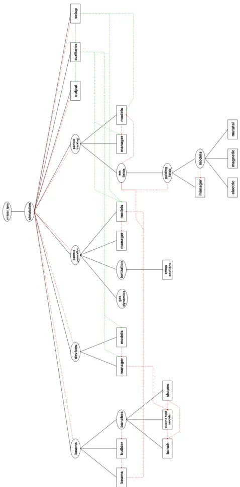
The application is organized as a Python package and each of the components is represented by a separate sub-package (with exception to theOutput Recorder component (section3.8) which is represented by a single module). The framework contains several auxiliary components mostly for storing and modifying particle data and for providing common configuration parameters. Figure2shows the structure of the package together with dependencies between the different components and figure3 shows the dependencies between the core components in detail. Figure4shows how those components interact with each other and what tasks they perform related to the simulation loop.
3.1. Model & Manager
Components which represent parts of the application that deal with (physics) problems and which can be addressed in multiple ways feature a concept ofmodelsandmanagers. Amodel is a specific implementation which addresses the problem in question and which provides the corresponding functionality that is required by a related (template) base class in order to fulfill a common interface. That means a model represents a particular solution for the given problem or aspect (e.g. a numerical Poisson solver is a model which provides a specific way of computing the bunch electric field). A manager wraps the corresponding model which is used for a particular simulation run and serves as an entry point for other parts of the framework (hence it can be seen as an adapter for the model which connects it to the rest of the framework). This structure intends to remove any (common) overhead from the specific solutions (the models) and transfers it to the managing component (the manager) which is the same for each model. Such overhead includes data conversions, coordinate transformations or other auxiliary tasks which are not directly related to a specific problem.
A model solves the particular problem in a preferably simple and isolated environment and the manager then connects this solution to the application.
3.2. Particle generation
AParticle Generation Model represents a way for particles to enter the simulation cycle. For IPM simulations this will most frequently incorporate the ionization process induced by the interaction of the particle beam with the rest gas. Nevertheless implementing other models can be easily realized. For example studying secondary electron emission emerging from
Figure 2: The structure of the software package also indicating the dependencies between
3.2. Particle generation
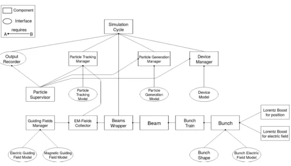
Figure 3: The dependencies between the different core components of the framework.
Figure 4: Flowchart showing the actions that take place during the “lifetime” of a particle.
Each step is handled by a separate component of the framework.
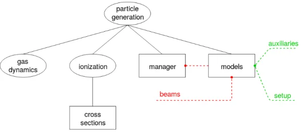
Figure 5: The structure of the particle generation sub-package. Another sub-package for handling tasks related to the gas dynamics is foreseen.
ion impact on detector elements (see section2.1.6) one would use a model which generates particles based on the output of a previous simulation run during which the ions were tracked towards the detector. In order to simulate an electron gun one could use a corresponding particle generation model which is based on measurements from a real electron gun and which generates electrons according to these distributions. The particle generation model is queried every simulation time step and asked to generate as many particles as appropriate for the given step. As mentioned in section2.2 each simulation run features exactly one particle generation model. If different particle types are to be analyzed this can be achieved by separate simulation runs. Figure5shows the structure of the particle generation sub- package. Besides the commonmodels andmanager modules it contains a sub-package for contents related toionization as for example ionization cross sections. Another sub-package which handles tasks related togas dynamics (becoming important for gas jet simulations for example) is foreseen. Particles are generated by invoking the appropriate methods on the Particle Supervisor component (section3.9.2) which is part of theauxiliaries module.
3.2.1. Ionization
For IPM simulations the most common way of generating particles is through ionization.
Two aspects are important:
• Initial positions which reflect the bunch’s charge distribution.
• Initial momenta emerging from the ionization process.
For the purpose of initial position generation the corresponding bunch shape instance (see section3.6.2) provides a method for sampling positions according to its (transverse) charge distribution. For the purpose of momentum generation a separate package for ionization cross sections was prepared [19] and the framework exposes several adapters for connecting the
3.3. Particle tracking
ionization cross section classes of this package to corresponding particle generation models.
Such an adapter class provides a method for generating momenta according to the underlying ionization cross section. Different ionization cross sections such as single differential or double differential ionization cross sections are available. In any case they define the energy and the (polar) scattering angle distribution of ionized particles and hence define the resulting momentum distribution.
3.3. Particle tracking
Particle Tracking Models are responsible for propagating particles during the simulation.
Each model must provide a method for updating the particles’ positions and momenta at a given simulation time step. Propagating particles is an action which needs to be performed per time step and per particle and therefore an efficient method is desirable. On the other hand accuracy of the tracking plays an important role too. This is usually controlled with a time step size ∆tby which particles are “pushed” during the current simulation step. A smaller ∆tusually implies higher accuracy but also a greater number of updates that need to be performed in total leading to prolonged simulation runs. Thus some kind of trade-off has to be made and an optimum has to be found. Usually it is a good indicator to check a few particle trajectories for different time step sizes and to observe when they converge. Once they do the time step size is reasonably small and can be used to perform a complete simulation run. More about this topic can be found in section5.1. Figure6shows the structure of the particle tracking sub-package. Because the electromagnetic fields determine the particles’
trajectories they are wrapped in another sub-package. This sub-package contains the guiding field models and declares a cross-reference to thebeams sub-package (section3.6) in order to incorporate the beam fields as well. The relevant particles (those to be tracked) are retrieved from theParticle Supervisor component (section3.9.2) hence the corresponding dependence.
3.4. Devices
On the one hand aDevice Model defines the spatial boundaries of the simulation (i.e. the relevant simulation region) and on the other hand it decides when the particles’ statuses should change because they are detected or invalidated (invalidated means a particle should stop tracking while it was not detected; e.g. because it hit other parts of the chamber than the detector). The boundaries are specified in the laboratory frame (the reference frame in which particle positions are measured) and this boundary information can be reused by bunch electric field models in order to confine the volume in which the electric field has to be precomputed (see section3.7.1). The task of identifying particles as being detected is a very general one and applies to all the presented use cases (section2.1). For example when studying a BIF monitor one would use a device model which computes the decay rate of excited states and the corresponding decay probability for each particle. The model then changes the particles’ statuses accordingly, based on a (pseudo-) random probabilistic sampling. Once a particle’s excited state is decayed the particle is marked “detected” and
Figure 6: The structure of the particle tracking sub-package.
Figure 7: The structure of the devices sub-package.
one can estimate the distance it has traveled and thus compute an influence on the measured beam profile. Figure7shows the structure of thedevices sub-package. In order to check only tracked particles and to change particle statuses a device invokes the corresponding methods of theParticle Supervisor component (section3.9.2).
3.5. Guiding fields
Guiding Field Models describe the external electric and magnetic fields which are applied in order to guide the particles towards the detector. Two kinds of guiding fields are considered, electric and magnetic guiding fields. The guiding fields may vary in time and each simulation run involves exactly one electric and one magnetic guiding field model (if different effects need to be stacked this should be done beforehand, “outside” of the simulation, by use of an appropriate joint model). Because the guiding fields are required for propagating particles
3.6. Beams
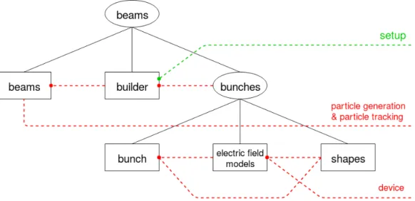
Figure 8: The structure of the beams sub-package.
during the simulation evaluating the fields is an action which takes place per simulation step and per particle and thus should be an efficient procedure. Figure6shows the structure of theguiding fields sub-package. Because of similarities between the electric and magnetic guiding field models their core functionality has been moved to a separatemixin module and the concrete guiding field models are created via (multiple) inheritance from both the mixin model (providing the functionality) and the specific template base class (providing contents relevant for configuration and setup of a simulation run).
3.6. Beams
Each simulation run involves an arbitrary number of beams. Beams take part in processes such as ionization as well as are accompanied by an electromagnetic field which influences the trajectories of particles. Because of this broad range of functionality a separate sub-package beams has been created for this component. By convention the bunches of a beam always
move in positive z-direction.
3.6.1. Bunch trains
ABunch Train describes the locations of bunches that are part of a beam. Specifically it defines the longitudinal offsets of bunches to the origin of the laboratory frame (the device center) which are used for coordinate transformations from the laboratory frame to a bunch’s rest frame.
Linear bunch train For aLinear Bunch Train all bunches are placed one behind another and they “move” through the simulation region as the simulation advances (this movement is rather virtual, their longitudinal offsets remains constant, but due to the four vector
transformation of particle positions this is equivalent to the bunches advancing in space).
Once a bunch leaves the simulation region it continues to travel in the same direction farther away until the simulation stops. Every two subsequent bunches are separated by the same positive (time-like) spacing. Because the fields of bunches which are farther away may be negligible the user may define awindow width which determines which bunches in the bunch train should be taken into account for the field evaluation (the window is centered around the device center); this potentially speeds up the simulation as beam field evaluation is computationally rather expensive because it is performed per simulation step and per particle.
Circular bunch train For aCircular Bunch Train the bunches are also placed one behind another but with the difference that they are “wrapped around” an (imaginary) boundary outside the simulation region once they reach it during the simulation. This boundary is defined by the number of bunches and their (time-like) spacing. The boundary is placed atz=N ·Σt/2 in the laboratory frame whereN is the number of bunches and Σt is the (time-like) spacing between two subsequent bunches. Because the bunch train is centered around the origin of the laboratory frame this implies that the “rightmost” bunch has a distance of Σt/2 from the boundary. For each simulation time step the actual positions of the bunches are computed by checking their total advancement at the given time step and by wrapping their longitudinal positions around the boundary. If they are wrapped around, they appear on a corresponding left boundary (symmetric with respect toz= 0), emulating new bunches coming in the synchrotron.
3.6.2. Bunch shapes
Bunch Shape Models describe the charge distribution of a bunch. They are mainly responsible for two aspects: ionization and electric field computation. With regard to the former aspect each bunch shape model must provide a method for sampling positions of ionized particles according to its transverse charge distribution for a given longitudinal slice (that is the z-coordinate is fixed). If particles need to be generated along the bunch (as it is the case for short bunches) then multiple slices can be used for that purpose. An additional method for doing a complete three dimensional sampling could be implemented as well however for the discussed use cases it is not necessarily required. Also for such a method one must provide a way of confining the sampling with respect to the z-coordinate because for a real device using a pressure bump for example such a confinement takes place (note that this confinement is time dependent in the bunch frame).
For most IPM simulations it will be sufficient to generate particles atz= 0 (in the laboratory frame) provided that the guiding fields do not change along the z-axis and that the resulting distribution is integrated along the z-axis. Because the conditions are similar along the z-axis it is not important where particles are created with respect to the laboratory frame.
Instead their positions relative to the bunch are important. Therefore it is of importance that the particles are created “along the bunch” (i.e. that their time distribution follows the
3.7. Beam fields
longitudinal charge distribution of a bunch).
With regard to electric field computation a bunch shape needs to expose its charge distribution so it can be reused by the bunch electric field model (e.g. a Poisson solver). It might also provide additional optional attributes such as standard deviations of a Gaussian distribution.
3.7. Beam fields
The beam fields are based on the electric field of bunches in their rest frames and are computed as described in this section. Because only non-relativistic particles are considered for the particle tracking the particles’ positions can be described in a single reference frame, the laboratory frame (see section2.2). The positions in a bunch’s rest frame can be obtained from the four-vector-positions in the laboratory frame via Lorentz transformation. Furthermore, because of the convention that bunches move along the z-axis, this transformation reduces to a simple Lorentz boost in z-direction (the primed coordinates denote the bunch rest frame):
ct0 =γ(ct−βz) (1a)
x0 =x (1b)
y0 =y (1c)
z0 =γ(z−βct) (1d)
Because each bunch in the bunch train has a different longitudinal offset to the origin of the laboratory frame, we need to replacect→c(t+ti0) where ti0 is the time-like longitudinal offset of bunchi. Those offsets are kept constant during the simulation (an exception is the circular bunch train for which the longitudinal offsets are wrapped around a defined window boundary during the simulation) and the appropriate position is obtained from the Lorentz boost. The spatial position in the bunch rest frame is used to evaluate the electric field and the corresponding electromagnetic field tensor is transformed back to the laboratory frame using another Lorentz transformation (note that the bunch magnetic field vanishes in the rest frame of the bunch). Because of the movement along the z-axis this reduces to (the primed coordinates denote the bunch rest frame):
Ex=γEx0 (2a)
Ey=γEy0 (2b)
Ez=Ez0 (2c)
Figure 9: Diagram showing how the electromagnetic field of a beam is obtained.
Bx=−βγ
c E0y (3a)
By =βγ
c Ex0 (3b)
Bz=Bz0 (3c)
3.7.1. Bunch electric field models
Bunch Electric Field Models are responsible for computing the electric field corresponding to a given bunch shape in the rest frame of the bunch. This can be based on analytical solutions for specific cases as well as numerical solutions for arbitrary charge distributions. For that purpose the model can use information from the underlying bunch shape either by accessing certain attributes (e.g. the standard deviations of a Gaussian shape) or by evaluating its
3.8. Output recorders
charge distribution from a corresponding method. A bunch electric field model must provide a method for retrieving the electric field evaluated at a given set of positions in the bunch frame. The resulting field of a bunch electric field model is normalized to a bunch charge that equals the elementary charge. The appropriate rescaling with the charge number and bunch population takes place in the corresponding method of a dedicatedBunchclass which wraps the electric field model and also applies the Lorentz boost.
3.8. Output recorders
Output Recorders are responsible for extracting information about (kinematic) particle data from the simulation, i.e. they are some kind of information sink for particle data (they propagate the desired information to external resources, usually files). One important aspect is that output recorders only deal with particle related information. This means if one wants to retrieve other information such as electric field maps, this information should be obtained by different means (for example dedicated scripts which evaluate the corresponding methods of the related models). Output recorders are subscribed to the status update stream of theParticle Supervisor component (section3.9.2) on which all particle status updates are published and a corresponding callback method is invoked for each status update. An output recorder can react on such status updates by implementing this callback method. In general monitoring particle information involves two aspects:
• Event-based information, such as status changes of particles (e.g. due to ionization or detection).
• Continuous information that must be queried periodically (e.g. particle positions for recording trajectories).
For the second purpose an output recorder’s record method is called after each iteration of the simulation loop is completed. This method can be overridden in order to periodically request particle data from the particle supervisor component.
3.9. Auxiliaries
3.9.1. Simulation cycle
ASimulation Cycle defines when a particular simulation run should terminate. The option which is currently available is a “fixed duration” cycle. That is the user specifies a simulation time and a number of time steps (which together define the time step size ∆t) and the cycle runs for the specified number of steps. Therefore it is up to the user to ensure that the specified simulation time is long enough in order to simulate all the effects that are part of the specific case (for example for a bunch with length 10 ns the simulation time should be larger than 10 ns in order to ensure that all particles are created due to ionization; some additional time should be considered for those particles to reach the detector).
Another possible option would be a simulation cycle that runs until all particles have been detected or invalidated. This would allow for using a variable time step size in form of adaptive particle tracking algorithms. The advantage of such tracking algorithms is that they have a better performance because they choose the time step size such that it fits the current field values and field gradients. A fixed time step size ∆t must be chosen generally small in order to ensure the field quality at any time during the simulation. An adaptive algorithm could increase ∆twhenever the fields or the field gradients are small.
Such a simulation cycle would strongly benefit from a way of generating particles that doesn’t involve “slicing” the simulation time as the simulation progress advances. The current implementation uses a “universal” simulation time that advances with the simulation progress (measured in number of elapsed steps). Models are then asked to perform their tasks for the current progress (for example a particle generation model should generate particles according to the beam’s charge density at the given universal simulation time).
However each particle already maintains a distinct (proper) time in form of the position four-vector and this time is deciding for the Lorentz transformations for example. Therefore the global simulation time could be dropped and the simulation would be described solely by its progress in number of steps. A particle generation model can then create all particles directly at the beginning of the simulation, distributing them properly in space and time.
This is advantageous also because if particles are created step-by-step it is not guaranteed that such a simulation cycle won’t terminate prematurely (due to no particles being tracked but others still “waiting” to be created).
3.9.2. Particle Supervisor
TheParticle Supervisor component is responsible for storing and modifying data related to particles. The data of all particles are stored together in numpy arrays [20] and the particle supervisor component provides ways of accessing this data. A Particle is a view onto a segment of those arrays and similarly aParticle Set is a view on a multitude of such segments (numpy’s array indexing is used for that purpose). Those views provide themselves methods for obtaining attributes such as position and momentum corresponding to the represented particles.
3.9.3. Setup
The auxiliarySetup component is used to declare universal parameters of the simulation which are the same for each setting, such as simulation time or the number of particles to be simulated. This component can be requested by other components in order to get access to those parameters. The parameters are unique to theSimulation Cycle (section3.9.1) and an additional simulation cycle class would also require an additional corresponding setup class.
3.10. Configuration
3.10. Configuration
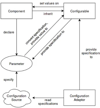
Many components need to be configured by means of specifying parameters such as beam energy or bunch population for example. The configuration should be handled automatically and should not be a major concern of components (especially models) of the application. For that reason the required configuration logic was moved to a separate Python package [21].
This package handles all the required tasks related to configuration. In the following, a brief overview of this configuration framework is given.
The framework uses the concept that components of the applicationdeclareparameters which are thenspecified by the user in a configuration source (usually a file). The configuration framework then handles the transfer of the specified values from the configuration file to the corresponding declaring component. While doing so it checks for any restrictions that were imposed during declaration of a parameter (for example accepting only positive integer values) and applies any necessary transformations (such as unit conversions for example).
Figure10illustrates the process of configuring components. In the following a brief overview of the available parameter types is given:
• Bool - An on/off parameter (switch); Example: Switch off the electric or magnetic field of a beam.
• String -Example: Filenames.
• Integer -Example: The number of bunches in a bunch train.
• Number - A floating point number;Example: The convergence limit for the Successive Over-Relaxation Poisson bunch field solver.
• Vector - A homogeneous list of an arbitrary parameter type (for example
Vector[Number]);Example: The transverse standard deviations of a Gaussian bunch shape.
• Duplet - A vector with two elements.
• Triplet - A vector with three elements.
• Tuple - A vector with an arbitrary fixed number of elements.
• PhysicalQuantity - Needs to be declared with a unit
(e.g. PhysicalQuantity(’Energy’, unit=’eV’));Example: Beam energy.
• Action - Must wrap another parameter and specify a custom action. The specified parameter value is transformed using this custom action. This parameter type also allows to declare dependencies on other parameters whose values are then passed as additional arguments to the specified custom action. Example: Particle types are specified by their charge number and rest energy and the corresponding instance is then created from the ParticleType class.
• Choice - Needs to be declared with a number of possible options; the specified value must be one of the declared options. Example: Names of gas types for ionization cross sections.
• Group - Must define a namespace and wrap a number of parameters. The wrapped parameters will appear under the defined namespace in the configuration source.
Example: The tracked particle type is specified by its charge number and rest energy.
• ComplementaryGroup - Must wrap a number of parameters. All but exactly one of the wrapped parameters must be specified by the user and the missing value is computed from the others using previously declared conversion rules. Example: Simulation time (T), time delta (∆t) and number of time steps (N). Each combination of two of those parameters defines the third one by the relation T =N·∆t.
• SubstitutionGroup - Must wrap a number of parameters, one of them which is marked
“primary”. Exactly one of the wrapped parameters must be specified and its value is converted to the corresponding primary parameter’s value using previously declared conversion rules. Example: The user can specify the bunch length either in the laboratory frame or in the rest frame of the bunch. If specified in the laboratory frame then the bunch length is appropriately converted, so the component receives the value in the bunch frame.
Components also need to declare where their parameters can be found in the configuration file. The framework checks this part of the file and retrieves the corresponding values. In the following an example for a Gaussian bunch shape is given:
@parametrize(
Duplet[PhysicalQuantity]('TransverseSigma', unit='m'), PhysicalQuantity('LongitudinalSigma', unit='s') )
class Gaussian(BunchShape):
CONFIG_PATH = 'BunchShape/Parameters'
@parametrize is used to declare the parameters “TransverseSigma” (in units of meters) and “LongitudinalSigma” (in units of seconds; measured bunch length in the laboratory frame). The class attribute CONFIG PATH specifies the location in the configuration file. The corresponding part of an XML configuration file would look like this:
<Beam>
<BunchShape>
<Model>Gaussian</Model>
<Parameters>
<TransverseSigma unit="um">[ 229, 257 ]</TransverseSigma>
<LongitudinalSigma unit="ns">1.25 / 4</LongitudinalSigma>
</Parameters>
</BunchShape>
</Beam>
The additional <Model> tag specifies that theGaussian bunch shape model should be used.
3.11. Start & Setup
Figure 10: Diagram showing the different aspects of configuring a component as realized by the configuration framework.
Note that the parameters are specified in different units than they were declared; the configuration framework knows the corresponding conversion rules and applies them so that a component always receives the parameters’ values as they were declared (that is for the given example in units of meters and seconds, respectively).
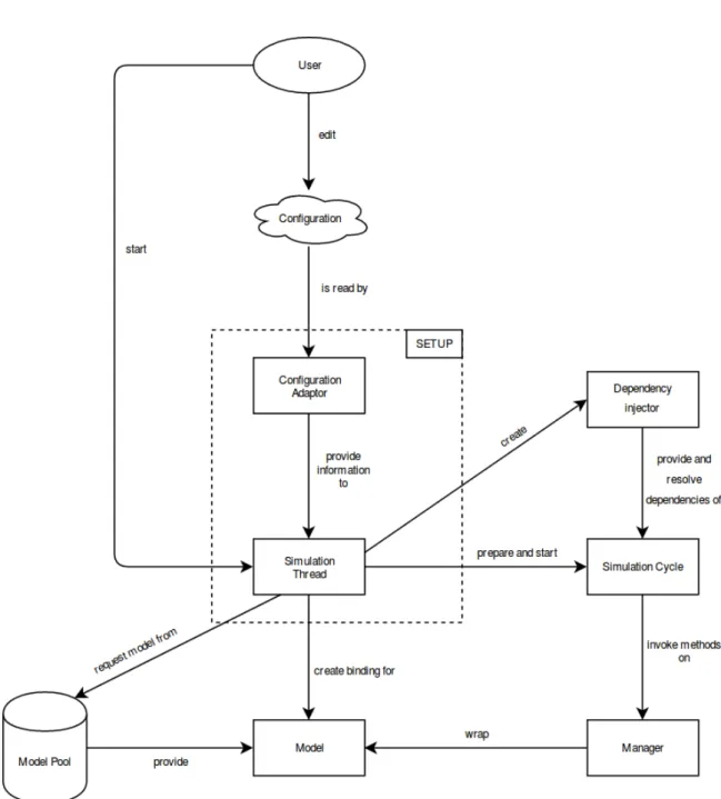
3.11. Start & Setup
In order to run a simulation the user must provide a configuration source (usually a configu- ration file). The configuration source must specify the models which should be used for the different modules (components) as well as all parameters that are declared by the involved models. The recommended way for doing this is by using the Graphical User Interface (GUI) (see sectionB.3) because it will guide the user through all the different parts of the
configuration process and notifies them in case of configuration errors.
The simulation can be started either from the GUI or from the command line (see sectionB).
When started from the GUI a separate simulation thread is created which instantiates the required models and starts the simulation cycle. The simulation thread provides information about the simulation progress and about particles via a publish/subscribe concept (using the ReactiveX library for Python [22]). The simulation GUI subscribes to the corresponding topics and hence provides real-time information about the simulation.
Figure 11: Diagram showing the actions that take place during the start and setup of a simulation run.
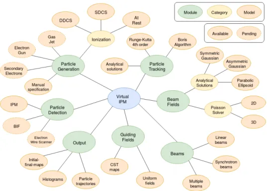
4. Available models
Figure 12: An overview of the available models. Dashed lines indicate future indented models which are not yet implemented.
4. Available models
Several different models have been implemented in order to address the previously mentioned components of the application. Some of these models were inspired or migrated from existing simulation codes for which they already proved successful. The following simulation codes served as a basis for migrating existing models:
• PyECLOUD-BGI[7] – An analytical solution for the equations of motion for specific configurations of the electromagnetic fields is used in this code (see section4.2.3). For the computation of the electric field of the beam this code uses an analytical formula for a two-dimensional elliptical Gaussian charge distribution (see section4.5.2).
• GSI-code[11] – This code uses an analytical solution of Poisson’s equation in three dimensions for a specific charge distribution (see section4.5.3).
• JPARC-code[8] – This code uses the Runge-Kutta 4th order algorithm for particle tracking (see section4.2.1) and a two-dimensional Poisson solver based on the Successive Over-Relaxation method for arbitrary charge distributions (see section4.5.4).
In the following an overview of the available and intended future models is given. Figure12 shows these models and to which module they belong.
4.1. Particle Generation
4.1.1. Single particle generation
TheSingleParticle model allows for placing a single particle in the simulation. The user can specify the time step as well as the initial position and velocity of the generated particle.
This is particularly useful for testing configurations by observing real-time trajectories of particles or for studying trajectories of specific particles in general.
4.1.2. Manual generation of particles
Multiple particles can be manually “placed” in the simulation by using theDirectPlacement model. The user can specify the simulation steps as well as the initial positions and velocities of the generated particles. This is particularly useful for studying the trajectories of specific particles under certain conditions (e.g. particles which are created at the head or the tail of a bunch). Also if one wants to study the influence of multiple bunches on the trajectories of tracked particles (most likely ions) then it is useful that only the first bunch ionizes all particles (as the situation is similar for following bunches). In order to do so one can run a single bunch simulation, convert the initial parameters from the output to the format of the Direct Placement model and then run a multi-bunch simulation with that parameters as an input.
4.1.3. Ionize particles at a fixed z-position
If the guiding fields of a device do not change along the z-axis and the resulting signal is integrated along this axis (while the profile along, for example, the x-axis is measured) then it is sufficient to generate all particles at a fixed z-position. Because the conditions are similar along the z-axis and for the beam fields only the relative positions of the tracked particles to a bunch are important we only need to make sure that the particles are properly distributed “along the beam”. This is achieved by fixing the z-position and distributing the particles in the time domain as the simulation advances, following the charge distribution of the beam for fixedz= 0 for example (note that a bunch’s time- and z-coordinate are coupled byz=βc(t+t0), wheret0is the bunch’s initial (time-like) offset to the device center). The momenta of ionized particles can be obtained with different methods. For example generating particles at rest or using ionization cross sections for estimating the momenta is available.
Figure13sketches how particles are distributed during the simulation for this approach.
This functionality has been implemented in theFixedZZeroMomentum,FixedZVoitkivDDCS andFixedZSimpleDDCS models which feature different methods for sampling the momentum.
4.1.4. Ionization cross sections
Ionization cross sections describe the energy and the scattering angle of products of ionization processes. Different types of cross sections - single and double differential ionization cross
4.1. Particle Generation
Figure 13: Sketch of how particles are generated atz= 0. The different colored distributions indicate the same bunch at different times during the simulation. The particles are sampled according to the distribution which is found atz= 0 for the given time step.
sections - have been implemented for the application.
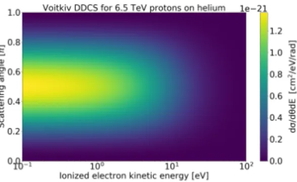
Double differential cross section (DDCS) The ionization cross section derived by Voitkiv et. al. [23] is applicable to the case of highly relativistic incident particles as well as projectiles with high charge numbers ((a)v/Zv2γ,1v < c or (b)Zv, v0v < c, in atomic units,Z being the charge number of the projectile). It is derived in a quantum mechanical approach by solving the non-relativistic Schroedinger equation with the help of Coulomb continuum wave functions for the case of hydrogen. An extension to helium is realized by the introduction of an effective charge as seen by the electrons in the 1s-shell of the helium atom. Therefore the applicability of this method to multi-shell atoms is questionable. The double differential cross section is given by the following expression [23, eq. (38)]:
d2σ(+1)He
dEdΩ = 2·28 Z2 v2Zt4
1
1 +2EZ2 t
5 exp
−
4 arctan r2E
Z2 t
r2E Z2 t
1−exp
−r2π
2E Z2 t
×
sin2θ·lnηHe+cos2θ
γ2 −0.5 sin2θ +8√
2E v cosθ·
1− v2
2c2
sin2θlnηHe+2ZZt
v2γ2 cosθln2ηHe
#
(4)
where Z is the charge number of the projectile, a0 is the Bohr radius, Zt is the effective charge of helium (determined to a value of 1.5),ηHe is a coefficient specific to helium,γ is the relativistic factor andv is the velocity of the projectile. The cross section is given in atomic units. Figure14 shows a plot of the cross section for 6.5 TeV incident protons on a helium target. The plot shows that most ionized electrons have small kinetic energies (E <10 eV) as it is typically the case for ionization by relativistic projectiles.
Figure 14: Double differential cross section for 6.5 TeV incident protons on a helium target.
Single differential cross sections (SDCS) For ionization by highly relativistic projectiles the interaction time is very short and the situation can be treated as a two-body problem;
the electron in the vicinity of the nucleus receives energy almost instantly in form of a short electromagnetic pulse originating from the rapidly varying electromagnetic field of the projectile (similar to photoionization). For those cases the main contribution to the ionized electron kinetic energy comes from the kinetic energy distribution of the bound electron.
Corresponding single differential cross sections (SDCS) have a typical shape which consists of a low-energy plateau part, representing the Compton profile of the target atom, followed by a slope which depends on the various shell contributions (see figure15). This plateau-slope shape can be parametrized by the four parametersσP (the plateau value of the SDCS),σS
(the SDCS value at the end of the slope),EP (the energy where the plateau ends and the slope starts) and ES (the energy where the slope ends); the plateau is assumed to start atE = 0. Note that this plateau-slope shape occurs in a log-log form and therefore the underlying distribution for the slope part is of the form
dσ dE
slope
= σP
EPa ·Ea , a= log (σS/σP)
log (ES/EP) (5)
The corresponding scattering angle distributions for ionization by highly relativistic projectiles typically have a Gaussian shape that is centered aroundθ=π/2. For projectile velocities close to the speed of light no “dragging” of the electron occurs during the ionization process (that is the electron would be accelerated in the direction of movement of the projectile) and therefore the skewness of the scattering angle distribution can be assumed to be zero. Figure 16shows the corresponding single differential cross section for 6.5 TeV incident protons on a helium target.
4.1.5. Electron gun (pending)
For studying electron wire scanners an electron gun needs to be emulated. A corresponding model could take a measured energy/emission-angle distribution as an input (from a data file or an analytical/numerical model for example) and use this distribution to generate electrons during the simulation.
4.1. Particle Generation
Figure 15: Single differential cross sections for 6.5 TeV incident protons on a helium target.
The blue curve shows the ionization cross section as derived by Voitkiv et. al. [23, eq. (39)]. The green curve represents a parametrization to reflect the typical plateau and slope part of such ionization cross sections. The values σP = 8.2×10⁻²¹, σS = 4.0×10⁻²³, EP = 8 eV, ES = 100 eV have been used for the parametrization.
Figure 16: Single differential cross sections for 6.5 TeV incident protons on a helium target.
The blue curve shows the ionization cross section as derived by Voitkiv et. al. [23, eq. (40)]. The orange curve represents a Gaussian fit to reflect the typical shape of the scattering angle ionization cross section.
4.1.6. Secondary electrons (pending)
Secondary electrons are generated from ions hitting the ion trap grid. In a first simulation run one would simulate the movement of ions towards the grid and record their impact positions and momenta. This output from a previous simulation run can then be used as the input to a secondary electron generation model which creates electrons according to a model which describes the interaction of impacting ions with the material of the ion trap.
4.1.7. Gas jet (pending)
A gas jet model incorporates ionization via the particle beam. Depending on the distribution of gas density in the jet the actual number of particles generated by the corresponding bunch shape model must be adjusted (rescaled) accordingly. The momenta of ionized particles are adjusted by supplying the velocity component of the gas jet itself. That is the ionized particles (ions or electrons) retain the velocity of the molecules in the gas jet.
4.2. Particle tracking
4.2.1. Runge-Kutta 4th order
The Runge-Kutta method is a general method for solving ordinary differential equations of the form
d
dty(t) =f(y(t), t) (6)
by bringing them into a linear form. Runge-Kutta methods exist of various orders which characterize the number of intermediate evaluations off(y, t) which are used to determine the “next” value of y(t). A starting point y0 ≡ y(t0) needs to be supplied. From this starting point on the next value ofy(t) is estimated by a linear update (linear int). This is achieved by discretizing the time domain. The following considerations refer to the 4th order Runge-Kutta method. For a finite update of length ∆tthe updated value ofy(t) is computed as:
yn+1=yn+∆t
6 (k1+ 2k2+ 2k3+k4) (7)