Dynamical Modeling of the Demographic Prisoner's Dilemma

IHS Economics Series Working Paper 124

November 2002

Dynamical Modeling of the Demographic Prisoner's Dilemma

Victor Dorofeenko

Jamsheed Shorish

Impressum Author(s):

Victor Dorofeenko, Jamsheed Shorish Title:

Dynamical Modeling of the Demographic Prisoner's Dilemma ISSN: Unspecified

2002 Institut für Höhere Studien - Institute for Advanced Studies (IHS) Josefstädter Straße 39, A-1080 Wien

E-Mail: o ce@ihs.ac.atffi Web: ww w .ihs.ac. a t

All IHS Working Papers are available online: http://irihs. ihs. ac.at/view/ihs_series/

This paper is available for download without charge at:

https://irihs.ihs.ac.at/id/eprint/1459/

Dynamical Modeling of the Demographic Prisoner's Dilemma

Victor Dorofeenko, Jamsheed Shorish

124

Reihe Ökonomie

Economics Series

124 Reihe Ökonomie Economics Series

Dynamical Modeling of the Demographic Prisoner's Dilemma

Victor Dorofeenko, Jamsheed Shorish November 2002

Institut für Höhere Studien (IHS), Wien

Institute for Advanced Studies, Vienna

Contact:

Jamsheed Shorish

Department of Economics and Finance Institute for Advanced Studies

Stumpergasse 56, A-1060 Vienna, Austria (: +43/1/599 91-250

fax: +43/1/599 91-555 email: shorish@ihs.ac.at

Victor Dorofeenko

Department of Economics and Finance Institute for Advanced Studies

Stumpergasse 56, A-1060 Vienna, Austria (: +43/1/599 91-183

fax: +43/1/599 91-555 email: dorofeen@ihs.ac.at

Founded in 1963 by two prominent Austrians living in exile – the sociologist Paul F. Lazarsfeld and the economist Oskar Morgenstern – with the financial support from the Ford Foundation, the Austrian Federal Ministry of Education and the City of Vienna, the Institute for Advanced Studies (IHS) is the first institution for postgraduate education and research in economics and the social sciences in Austria.

The Economics Series presents research done at the Department of Economics and Finance and aims to share “work in progress” in a timely way before formal publication. As usual, authors bear full responsibility for the content of their contributions.

Das Institut für Höhere Studien (IHS) wurde im Jahr 1963 von zwei prominenten Exilösterreichern – dem Soziologen Paul F. Lazarsfeld und dem Ökonomen Oskar Morgenstern – mit Hilfe der Ford- Stiftung, des Österreichischen Bundesministeriums für Unterricht und der Stadt Wien gegründet und ist somit die erste nachuniversitäre Lehr- und Forschungsstätte für die Sozial- und Wirtschafts - wissenschaften in Österreich. Die Reihe Ökonomie bietet Einblick in die Forschungsarbeit der Abteilung für Ökonomie und Finanzwirtschaft und verfolgt das Ziel, abteilungsinterne

Abstract

Epstein (1998) demonstrates that in the demographic Prisoner’s Dilemma game it is possible to sustain cooperation in a repeated game played on a finite grid, where agents are spatially distributed and of fixed strategy type (‘cooperate’ or ‘defect’). We introduce a methodology to formalize the dynamical equations for a population of agents distributed in space and in wealth, which form a system similar to the reaction-diffusion type. We determine conditions for stable zones of sustained cooperation in a one-dimensional version of the model.

Defectors are forced out of cooperation zones due to a congestion effect, and accumulate at the boundaries.

Keywords

Prisoner’s dilemma, demographic, active media, reaction-diffusion

JEL Classifications

C61, C73

Comments

Contents

1 Introduction 1

2 The Model 3

2.1 The Demographic Prisoner's Dilemma...3

2.2 Formalization of the Model...5

3 Continuous Approximation and Dynamics 7

4 Numerical Solution and Qualitative Analysis 11

4.1.1 Homogeneous Steady-State Solutions and Stability... 12

4.1.2 A Linear System... 14

5 Conclusions and Future Research 15 6 Appendix 17

6.2 Boundary Condition at w = 0... 17

6.3 Solution with Constant Coefficients ... 18

6.4 The Argument Principle ... 20

References 22

7 Figures 23

1 Introduction

Computational economic modeling is often performed using the cellular automata ap- proach (see e.g. von Neumann 1966, Wolfram 1994). Economic agents are placed in a spatial grid at discrete nodes, and their behavior is influenced by the environment of each agent, i.e. the surrounding neighborhood in the grid. Agents may traverse the grid according to pre-defined rules, so the framework has the advantage of allowing re- peated economic interaction to affect the entire population of agents. At the same time, individual interaction is restricted to a limited area.

This approach has recently been used by Epstein (1998) to model the traditional Prisoner’s Dilemma problem in a spatial, ‘demographic’ framework. Epstein demonstrates that if the outcome of pairwise Prisoner’s Dilemma encounters without memory affects the survivability and procreation of agents on a grid, then there may form spatial structures (known as ‘zones of cooperation’) which persist over time. These zones of cooperation are simply collections of agents who play the ‘cooperative’ strategy of the Prisoner’s Dilemma game. This is a novel result, as previous literature on the repeated Prisoner’s Dilemma in memoryless game environments predicts that agents who play the cooperative strategy will die out over time, i.e. only those agents who play the ‘defecting’ strategy will survive.

In games with memory, however, such zones of cooperation may often exist (Lindgren 1996).

The cellular automata mechanism, combined with a probabilistic choice of the events which occur at each ‘time step’ of the model, generates a spatial representation of an evolutionary process (in this case, the evolution of strategy types of collections of agents).

In principle, this could allow one to calculate analytically the time dependence of mean values of the population (e.g. the relative population shares of cooperators vs. defectors, the level of wealth, birth rate, etc.). Unfortunately, the calculation of the probability

1See, for example, Weibull (1995) and Samuelson (1997) for classical evolutionary game theory, and also Epstein (1998)’s discussion of evolutionary game theory and replicator dynamics.

distribution functions of the underlying parameters, and hence of the mean values them- selves, is notoriously difficult and requires extensive computational resources. Indeed, Epstein’s analysis relies instead upon a set of numerical simulations, using many time step iterations to demonstrate the existence of sustained zones of cooperation.

The purpose of this paper is to propose a formal framework for such spatial models, based upon the dynamical equations governing the evolution of the probability density functions for each type of agent. We apply this approach to the demographic Prisoner’s Dilemma in order to arrive at analytical equations which govern the evolution of the system. These equations, although continuous in nature, may be derived from the cellular automata model as the spatial grid step and the payoff received (or lost) by an agent in a single-game interaction become sufficiently small.

In order to derive these equations we presume a form of ‘statistical independence’ be- tween agents. This independence, which captures the essential feature of local interaction within the grid, allows us to obtain the equations for a single agent’s probability density function. To help render the admittedly complicated dynamical equations in the simplest light possible, we numerically solve a one-dimensional spatial model (in which agents are placed along a line). This model still captures the local interaction-global interaction dichotomy exemplified in Epstein’s two-dimensional spatial grid.

We demonstrate that the numerical solutions of the dynamical equations indicate sustainable zones of cooperation, as Epstein showed in the discrete grid environment.

The space-time evolution of a given agent’s wealth distribution is also observed. We show qualitatively that one reason for the existence of sustainable zones of cooperation is a congestion effect, which is a type of competition for scarce resources (in this case, the finite space of the grid). This competition is not only between existing agents for ‘living space’, but is also between agents who seek locations to produce offspring (which are of the same strategy type as the ’parent’ agent.)

2

The qualitative analysis demonstrates that the congestion effect allows sustainable zones of cooperation to persist, by displacing defectors from those locations with a high density of cooperators. This effect is implicitly contained in Epstein’s discrete framework.

But the kinetic approach used in this paper provides a useful framework for both explicit formalization and qualitative interpretation of the underlying dynamical equations, so that effects like congestion may be rigorously treated.

The paper is organized as follows. Section 2 introduces both the original model of Epstein and the formalization of this model in terms of the dynamical equations. Section 3 then introduces and qualitatively describes the continuous approximation of the model.

Section 4 provides a numerical solution of this system, and develops further qualitative analysis of two simple versions of the general equations. Section 5 concludes and dis- cusses future research, while the Appendix provides more detailed calculations for the formalization and the continuous approximation.

2 The Model

2.1 The Demographic Prisoner’s Dilemma

We begin by introducing Epstein’s demographic Prisoner’s Dilemma model on a discrete grid. Agents are assumed to be spatially distributed over an n-dimensional cube, which is partitioned into discrete points.

Each agent is located at one of several equidistant nodes x

= (i

δ, i

δ, ..., i

δ), where δ > 0 is the grid step and i

, i

, ..., i

take integer values between 0 and N > 0.

An agent’s behavioral strategy consists of randomly selecting a nearby node and then playing one round of a Prisoner’s Dilemma game if that node is occupied by another agent

2We generalize Epstein’s original two-dimensional model tondimensions, as the formalization given in the next section accommodates any spatial system of finite dimension.

(see Table 1 for an example of the Prisoner’s Dilemma payoff matrix which is used in the numerical solution.) The probability that an agent chooses a node during an infinitesimal time interval dt is g dt, where the time rate g is assumed to be constant.

The agent’s fixed (pure) strategy, which is played for life, defines the type i of an agent: i = c when an agent plays the strategy ‘cooperate’, while i = d if an agent plays the strategy ‘defect’. Each agent is also endowed with a level of wealth w. Conditional upon the types of the agent and his opponent, the game payoff after playing the game is then the change in the agent’s current wealth level. We define the game payoff as

∆w

, i, j = c, d. This is the amount of wealth added to (or subtracted from) the current agent’s wealth w when the agent’s type is i and the opponent’s type is j.

After playing a strategy, the agent moves to a new node. The agent randomly selects a nearby node to move to with a constant time rate m. If the node chosen is empty, the agent jumps there–otherwise, the agent remains in place.

An agent can produce an offspring if his wealth exceeds an exogenously determined threshold level w

. This birth process is similar to the play and movement processes discussed above. A random nearest node is chosen by an agent with the constant time rate b and, if it is empty, an offspring is produced and placed there. The initial newborn’s wealth, w

, is distributed according to an exogenous probability density function f

(w

).

The ‘parent’ agent loses a fixed amount of wealth ∆w

in the birth process. The strategy of the offspring is identical to the strategy of the parent.

Finally, an agent dies in an interval dt with a probability d · dt, where the time rate d is constant. In addition, an agent dies if his wealth w becomes negative. This model is thus sensitive to a translation of the zero of the wealth scale.

4

2.2 Formalization of the Model

To formalize the model it is very useful to consider an empty node as a special type of agent. Each agent’s state is defined by the agent’s type i = c, d, e (cooperator, defector or empty node), an n-dimensional spatial location at the grid x and the wealth w. For brevity we let q := (w, x). The total number of agents is thus equal to the total number of nodes N

< ∞, and is a constant.

We define functions F

(t, q

, ..., q

) , s ≤ N

such that

F

(t, q

, ..., q

) dw

dw

...dw

(1)

is the probability to find s agents of types i

, ..., i

in the state q

, ..., q

at the time t. The function F

is symmetric with respect to the permutation of arguments q

, q

, 1 ≤ i, k ≤ s. Since an empty node is considered formally as a special type of agent, all the processes excluding death (i.e. movement, playing and reproduction) can be treated as two-agent interactions. We also assume that the state variables q, q

of any two agents are pairwise independent, i.e.

F

(t, q, q0) ≈ F

(t, q) F

(t, q0) . (2)

The dynamic equations for the cooperator and defector functions F

(t, x, w) := F

(t, q), i = c, d follow from Section 2 and have the form

3Intuitively, this assumption states that correlations between two agents occur at the distance of the grid step δ, over which an agent’s probability density function remains (nearly) unchanged. Taking into account the oscillatory nature of the pair correlation function, one may then expect that correlations will vanish after averaging over a region of space much larger than a factor ofδ.

∂Fi(t,q)

∂t

= −dF

(t, x, w) + bn

(t, x) n

(t, x) f

(w) +

P

j=c,d

P

∆x=±1

[F

(t, x, w − ∆w

) − F

(t, x, w)] n

(t, x + ∆x)

+

P

∆x=±1

[θ (w + ∆w

− w

) F

(t, x, w + ∆w

)

−θ (w − w

) F

(t, x, w)] n

(t, x + ∆x)

+

P

∆x=±1

[F

(t, x, w) n

(t, x + ∆x) − F

(t, x + ∆x, w) n

(t, x)]

(3)

where the spatial densities of agent types are defined as

n

(t, x) = Z

wb

F

(t, x, w) dw, n

(t, x) = 1 − X

k=c,d

n

(t, x) , n

(t, x) =

Z

0

F

(t, x, w) dw,

the total agent density equals the (constant) grid node density and is normalized to 1, and finally

θ (x) =

 



 

1 x > 0 0 otherwise

. (4)

Briefly, equation (3) describes the dynamics of a single agent’s probability density function, which is a type of continuous time Markov equation. Each positive (negative) term on the right-hand side of (3) defines the possible transition to (from) the current state q = (x, w) and corresponds to one of the four basic processes in the system. These processes are:

6

1. an agent’s occasional death, occurring at a rate d, 2. the birth of a new agent at a rate b,

3. the inflow and outflow of agents due to a change in their wealth w, either as an outcome of the Prisoner’s Dilemma game or due to the birth of a new agent (these are terms proportional to g and b, respectively), and

4. the inflow and outflow of agents due to a change in their location x when moving (terms proportional to m).

Note that the agents’ pairwise interactions make the transition probabilities depend upon the agents’ spatial densities, so that equation (3) is nonlinear.

3 Continuous Approximation and Dynamics

Consider the continuous functions f

(t, x, w) which coincide with F

(t, x, w) at the discrete grid points x = iδ and satisfy equation (3) at any real (not just discrete) value of x. If these functions change only a little after a small set of transitions (q

, q

) → (q, q0), they can be expanded in a Taylor series in ∆q = q0 − q, ∆q

= q

− q, ∆q

= q

− q.

Using the series expansion up to second order in ∆q, ∆q

and ∆q

, we obtain

∂f

∂t + V

(t, x) ∂f

∂w − M

(t, x) ∂

f

∂w

− K (t, x) ∆

f

= (5) bn

(t, x) n

(t, x) f

(w) − [d + κ∆

n

(t, x)] f

,

where ∆

= P

i=1 ∂²

∂x²_i

is the Laplace operator, the coefficients V

(t, x) , M

(t, x) and

K (t, x) are nonlinear functions of the spatial densities of agents,

V

(t, x) = X

k=c,d,e

v

n

(t, x) , (6)

M

(t, x) = X

k=c,d,e

µ

n

(t, x) , K (t, x) = κn

(t, x) ,

and finally the constants v

, µ

and κ are functions of the rates of birth, movement and playing:

v

=

 



 

g∆w

, k = c, d

−b∆w

, k = e

, µ

= 1 2

 



 

g∆w

, k = c, d b∆w

, k = e

, κ = m 2 ∆x

.

Note that the coefficients v

depend upon both the payoff ∆w

of the game played and the wealth ∆w

lost in the birth process. Coefficients v

< 0 correspond to the wealth lost from a birth of a new agent (the rate of the process is proportional to the density of empty nodes n

). Coefficients v

> v

> 0 and v

< v

< 0 are proportional to the corresponding payoffs of the Prisoner’s Dilemma game.

To derive the boundary condition at w = 0, assume that in the region w < 0 the death rate d = D is large and the birth rate b = 0. Then one can show using the boundary conditions

w→±∞

lim f

(t, x, w) = 0, f

(t, x, w)|

= 0, ∂f

(t, x, w)

∂w

¯ ¯

¯ ¯

w=+0 w=−0

= 0 (7)

that lim

f

(t, 0, x) = 0 (see Appendix).

Thus the boundary conditions for system (5) for the interval w ∈ [0, ∞) are

f

(t, x, 0) = 0, lim

w→∞

f

(t, x, w) = 0 (8)

8

A further simplification of the system (5) arises from the observation that the solutions of (5) demonstrate the same qualitative behavior when the coefficients M

and K are treated as constants, and the term κ∆

n

(t, x) is omitted (see the discussion below).

The number of parameters of (5) can thus be reduced by means of the following scale transformations:

bt → t, q

Mi

w → w, q

b

K

x → x, q

Mi

b

f

→ f

,

d

b

→ d,

i

→ V

, q

b

f

³q

b

w

´

→ f

(w) Using this, the system (5) can be rewritten as

∂f

∂t + V

(t, x) ∂f

∂w − ∂

f

∂w

− ∆

f

= n

(t, x) n

(t, x) f

(w) − df

, (9) for i = c, d, e.

We note that the integro-differential system (9) is quite similar to that of the reaction- diffusion type (see e.g. Kerner and Osipov 1994). However, the nonlinear item V

(t, x)

and the non-local dependence of the right-hand side of the system on f

are markedly different from a standard system of the reaction-diffusion type.

3.1 Interpretation of the Simplified System (9)

It is possible to give a straightforward interpretation of the system (9) by considering

the overall effect of each term on the dynamical evolution of agent types. First, the

term V

(t, x)

is responsible for the permanent shift of the function f

(t, x, w) along

the wealth coordinate w, with the speed V

(t, x). Taking the first two terms together,

we can write the solution of the equation

+ V

= 0 as f = f (w − V t), which shows

this propagation of the density function in the wealth coordinate over time. Note that

according to (6) the nonlinear speed V

depends upon both the mean payoff of the game

played and the mean wealth lost in the birth process.

In addition, the terms

and ∆

f

result in the diffusion of f

(t, x, w) along the wealth and spatial coordinates, respectively. The typical solution of the equation

−

∂²f

∂w²

= 0 is f =

exp

³

−

´

and presents a gradually “dissolving” function, the maxi- mal value of which decreases in time as

while the width increases as √

t. This implies that n = R

f dw remains constant. The diffusion along the spatial coordinate results from the Brownian-motion-like spatial movement of the agents. The diffusion in wealth follows from the fact that the wealth of an agent after playing a game changes by a small but finite discrete step (the game’s payoff). These effects are known in the computational physics literature as a “grid diffusion” (see e.g. R. P. Fedorenko, 1994).

The terms on the right-hand side of (9) show the change in the number of agents for a given type. The term n

(t, x) n

(t, x) f

(w) leads to the birth of new agents with initial wealth distributed as f

(w). The birth rate, n

(t, x) n

(t, x), is proportional to both the mean spatial density of “adult” agents (whose wealth is greater than the threshold w

), n

(t, x), and the density of free cells, n

(t, x). This dependence upon the density of free cells represents a congestion effect, which we identify as one of main contributing factors to the zones of cooperation which arise in the demographic Prisoner’s Dilemma (see the following Section). Lastly, the term −df

is responsible for the decrease in the population of agents of type i due to the death process.

The balance equations for 1) the population share of each type of agent, N

(t), and 2) the mean wealth levels of each type of agent, W

(t), are located in the Appendix.

4Note that the balance equation for the population sizeN, which takes the form ^dN_dt = (1−CN)N, is known in theoretical ecology as the logistic equation and describes ecological systems with inter- and intra-species competition for resources (e.g. free space). See Svirezhev (1987).

10

4 Numerical Solution and Qualitative Analysis

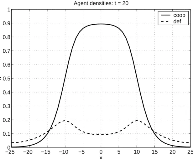
The numerical solution of system (9) with boundary conditions (8) for a one-dimensional version of the model (i.e. n = 1) is shown in Figure 1, and demonstrates the formation of a cooperator “colony” surrounded by a layer of defectors. The payoff matrix for the Prisoner’s Dilemma game used in the solution is shown in Table 1. The density of defectors is maximal at the border of the cooperator colony and decreases both to the center of colony and outward. Unlike Epstein’s discrete model, the density of defectors does not vanish, but only decreases over time.

c d

c 3.0,3.0 -18.0,6.0 d 6.0,-18.0 -17.4,-17.4

Table 1: Payoff matrix for the Prisoner’s Dilemma game used in numerical solution. (c) = cooperate, (d) = defect

The persistence of the cooperator colony lies in the fact that the density of cooperators is so high in the center of the colony that defectors are ‘locked out’, i.e. they cannot exploit the wealth of cooperators in the center of the zone. In addition, the cooperator colony cannot disperse, or diffuse throughout the spatial grid, as the defector population surrounds the cooperator colony and prevents its diffusion. This again keeps the internal density of cooperators within the zone high enough to prevent defectors from entering.

The inability of defectors to create their own colony follows from the negative payoff

of the defector-defector game (Epstein 1998). Their survival is solely due to the existence

of the cooperator colony. As mentioned before, the high density of cooperators in the

central part of the colony prevents defectors from excessive reproduction. This is due to

a congestion effect –there is simply not enough room with adequate contact with the co-

operator colony for many defectors to survive. In addition, the low density of cooperators outside of the zone prevents defectors from acquiring enough wealth to reproduce and fill the rest of the ‘empty’ areas.

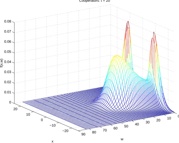
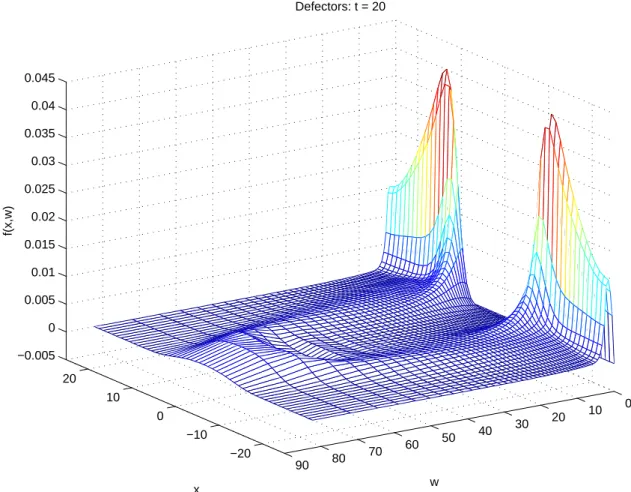
Thus, the combined effects of congestion and limited reproduction is the reason for the spatial dependence of the population densities of both defectors and cooperators upon the spatial grid. This dependence is evident in the numerical solutions for the population densities, which are presented in Figures 1 - 3. Figure 1 presents the probability density functions of cooperators and defectors, averaged over wealth. The zone of cooperation is clearly evident here, as is the accumulation of defectors on the ‘edge’ of the zone. Figures 2 and 3 show the full dependence of the probability density functions on both the spatial coordinate and the wealth level, for cooperators and defectors, respectively.

4.1 The Qualitative Structure of Two Simple Systems

In this section we consider some special and simplified cases of one-dimensional version of system (9) to get an improved qualitative picture of the process. In particular, we assume that the new-born wealth is a constant w

, so that f

(w) = δ (w − w

), where δ (x) is the Dirac delta function. We also set the birth threshold w

= w

. Then system (9) may be rewritten as

∂fi

∂t

+ V

(t, x)

−

−

+ df

= 0 f

(t, x, w)|

= 0,

¯ ¯

¯

w0−0

= −n

(t, x) n

(t, x) , (10) for each i = c, d, e.

4.1.1 Homogeneous Steady-State Solutions and Stability

The stability of the trivial steady-state solution f

(x, w) = 0 is treated as follows. The linearization of (10) f

= A

(w) exp (pt − ikx) yields

12

f

= C

 



 

[exp (µ

w

) − exp (µ

w

)] exp [µ

(w − w

)] w > w

exp (µ

w) − exp (µ

w) w ≤ w

where C is an arbitrary constant, the parameters µ

are

µ

= |v

| 2

"

−1 ± s

1 + 4 (p + k

+ d) v

# ,

p is defined by the formula

p = v

4

¡ s

− 1 ¢

− k

− d, (11) and finally s is a root of the equation

v

2 s (1 + s) = 1 − exp (−w

s) , (12)

with Re (s) > 0.

Standard analysis using the Argument Principle (see Appendix) leads to the conclusion that the unstable solution (11) is non-oscillatory, i.e. that p is a positive real number, if the following conditions hold:

w

> 1 s

ln 1

1 −

s

(1 + s

) , s

= s

1 + 4d

v

(13)

The inequality shows that the population will definitely grow from the zero level, if

the cost of birth is not too high and the initial wealth endowment of newborns is large

enough. Another consequence of (11) is that the maximal growth rate corresponds to the

homogeneous mode with k = 0. (This does not mean, however, that this property will

hold at the nonlinear stage of the evolution.)

4.1.2 A Linear System

We now turn to another simplification of the model, in which a linear version of system (10) is derived. This provides, as before, a method of analyzing this complicated system from a qualitative viewpoint, given the additional restrictions required. The linear version is obtained by considering system (10) for constant V

and n

. We derive the solution with the initial condition at t = 0:

f

(0, x, w) =

 



 

βn

(x) exp [−β (w − w

)] w > w

,

0 otherwise

(14)

In the asymptotic case V

À n

+ L

+ d and t À V

, the approximate solution of (10) (when V > 0) for the Fourier component

f

(t, w) = 1 2π

Z

−∞

f

(t, x, w) exp (−ikx) dx (15) is (see Appendix):

f

' K

 



 

exp £

−

(w − w

) ¤

if w > w

, exp [V (w − w

)] − exp ¡

−V w

−

w ¢

otherwise

(16)

where

K = n

n

V exp £¡

n

− k

− d ¢ t ¤

. (17)

In the periodic case k takes discrete values ±

, l = 1, 2, 3, ... and otherwise is a contin- uous variable.

Note that if V < 0, the solution decreases in time ∼ exp

³

−

t

´

and the population actually vanishes when t >

.

The dependence on t explains the time dynamics of the colony formation. The time rate n

− k

− d contains terms responsible for birth, n

, diffusion, −k

and death, −d.

14

If the birth rate n

exceeds the death rate d and the spatial size of the perturbation L ∼ k

is not too small, the population increases in time until the density of free cells n

= 1 − n

− n

decreases and the time rate vanishes. If the initial population of cooperators is significantly greater than that of defectors, then the cooperators will dominate in a “demographic explosion”.

However, in the regions with a lower density of cooperators, the population of defectors will grow faster. This results in a decrease in the cooperator’s wealth growth rate V

, leading to a decrease in the reproductive population share of cooperators with w > w

. The cooperator’s population then declines, and in fact this process leads to the total death of cooperators in the region where their population share is simply not high enough to sustain survival.

The factor f

, which depends upon the wealth of the agent’s type, is presented in Figure 4 for two values of V . This graph demonstrates that the share of reproductive agents decreases if V decreases, for levels of wealth larger than some critical value.

5 Conclusions and Future Research

The formalization of Epstein’s demographic Prisoner’s Dilemma introduced here has demonstrated that it is possible to both formulate and approximate the underlying dy- namical equations for spatial models of this type. Using the kinetic equation method under the assumption of statistical independence of agents, the continuous approxima- tion of the dynamical equations allows us to derive a relatively simple system of equations for the model. In addition, the derived system is similar to a reaction-diffusion process, and techniques which have been developed for analysis of such systems have been applied here.

The numerical solution shows that agent interaction in the demographic Prisoner’s

Dilemma results in the formation of sustained spatial zones of cooperation, as in Epstein’s original spatial model. The qualitative analysis of the kinetic equations indicates the influence of different factors of the model on this process. In particular, the congestion effect plays an important role in the formation of the zone, and can be interpreted as a form of implicit competition between agents for scarce resources (in this case, free space).

We wish to note that what has been done in this formalization is to approximate a cellular automata system by a kinetic system. This allows one to immediately calculate the spatial distribution of statistical means, independently of the size of the system. By contrast, the cellular automata approach yields the solution for the current realization, and the statistical analysis can then be performed by means of repeated calculations.

These repeated calculations may become computationally costly as the dimension of the model (e.g. grid size, population size, etc.) becomes very large.

More research is necessary to fully understand the parallels between the cellular au- tomata and the kinetic approaches, in order to better assess the strengths and weaknesses of each approach. This paper has been one step in this direction, in which a spatial system’s underlying dynamical equations have been formally stated, approximated, and solved (either numerically for the full model, or explicitly for simpler versions of the model). The results presented here at least show that the sustained zones of cooper- ation discovered by Epstein may be faithfully reproduced by the underlying dynamical equations, and are indeed a consequence of them.

16

6 Appendix

6.1 Balance Equations

The balance equations for the agent share N

(t) = R

−L/2

dx R

0

f

dw and the mean wealth of an agent W

(t) = N

(t) R

−L/2

dx R

0

wf

dw follow from (9) and have the form

dN

dt =

Z

−L/2

n

(t, x) n

(t, x) dx − dN

− Z

−L/2

∂f

∂w

¯ ¯

¯ ¯

w=0

dx, (18)

d

dt (N

W

) =

Z

−L/2

n (t, x) V

(t, x) dx + W

Z

−L/2

n

(t, x) n

(t, x) dx − dN

W

,

where W

= R

0

wf

(w) dw is the mean wealth endowment of a new agent, and R

−L/2

(...) dx denotes an integration over the n-dimensional spatial cube.

The negative term − R

−L/2

∂f

∂w

¯ ¯

w=0

dx represents the agent’s death at the border w = 0, when the agent’s wealth runs out. The interpretation of other terms is clear.

6.2 Boundary Condition at w = 0

The equations for the functions f

(t, x, w) if w < 0 are

∂f

∂t + V

∂f

∂w − ∂

f

∂w

− ∆

f

+ Df

= 0. (19) The asymptotic solution of (19) satisfying the boundary condition f

(t, x, w)|

= 0 if D À 1 is

f

(t, x, w) = h

(t, x, w) exp ¡

D

w ¢

, (20)

where h

(t, x, w) satisfies the equation

∂h

∂w − 1

2 h

− 1 2D

µ ∂h

∂t + V

∂h

∂w − ∂

h

∂w

− ∆

h

¶

= 0

and can be expanded in an asymptotic series in D

. The substitution of (20) into boundary conditions (7) yields

f

(t, x, w)|

= h

(t, x, 0) , ∂f

(t, x, w)

∂w

¯ ¯

¯ ¯

w=+0

= ∂h

(t, x, w)

∂w

¯ ¯

¯ ¯

w=0

+ D

h

(t, x, 0) ,

or

f

(t, x, w)|

= D

µ ∂f

(t, x, w)

∂w

¯ ¯

¯ ¯

w=+0

− ∂h

(t, x, w)

∂w

¯ ¯

¯ ¯

w=0

¶ .

Taking the limit D → ∞, we obtain f

(t, x, w)|

= 0.

6.3 Solution with Constant Coefficients

Consider equation (10), assuming V

and n

to be exogenous constants. The Laplace transformation on t and the Fourier transformation on x

f e

(p, k, w) = 1 2π

Z

0

exp (−pt) Z

−∞

exp (−ikx) f

(t, x, w) dxdt yield the ordinary differential equation

d

f e

dw

− V

d f e

dw − ¡

p + k

+ d ¢ f e

= −f

(0, w) , (21) with boundary conditions

f e

(p, k, 0) = 0, f e

(p, k, w)

¯ ¯

¯

= 0, (22)

18

f e

(p, k, w)

¯ ¯

¯

w0−0

= 0, ∂ f e

(p, k, w)

∂w

¯ ¯

¯ ¯

¯

w0+0

w0−0

= −n

Z

w0

f e

(p, k, w) dw, (23)

where f

(0, w) =

R

−∞

exp (−ikx) f

(0, x, w) dx.

In the special case

f

(0, w) =

 



 

βn

(k) exp [−β (w − w

)] w > w

,

0 otherwise,

(24)

the solution of equation (21) satisfying zero boundary conditions at w = 0 and w → ∞ (22) is

f e

(p, k, w) =

 

 



 

 

A

exp [λ

(w − w

)] +

p+k²+d+βVi−β²

w > w

, B

[exp (λ

w) − exp (λ

w)] w < w

,

(25)

where λ

=

± q

4

+ p + k

+ d, and A

and B

are constants. To define A

and B

, substitute (25) into (23) and solve the resulting linear system:

B

= βn

(k)

p + k

+ d + βV

− β

· (n

/β − λ

) (β + λ

)

n

[exp (λ

w

) − exp (λ

w

)] + λ

exp (λ

w

) (λ

− λ

) ,

A

= [exp (λ

w

) − exp (λ

w

)] B

− βn

(k)

p + k

+ d + βV

− β

.

The inverse Laplace transformation defines the Fourier component f

(t, w) of the function f e

(p, k, w)

f

(t, w) = 1 2πi

Z

σ−i∞

f e

(p, k, w) exp (pt) dp,

where the integration path in the complex plane for p, Re(p) = σ, is chosen to the right from all singularities of the function f e

(p, k, w).

According to the Residue Theorem, the last integral equals the sum of residues of f e

(p, k, w) exp (pt), which are calculated at the poles of f e

(p, k, w):

n

[exp (λ

w

) − exp (λ

w

)] + λ

exp (λ

w

) (λ

− λ

) = 0, (26)

p + k

+ d + βV

− β

= 0, (27)

and the integral along the both sides of the branch cut of f e

(p, k, w):

V

4 + p + k

+ d ≤ 0, Im(p) = 0. (28)

For simplicity we restrict our study to the case where V

À 1, β ∼ 1. Then the terms defined by (27) and (28) decrease rapidly in time as exp (−βV

t) and exp

³

−

t

´ , respectively, and can be omitted. The equation (26) has the approximate root

p ≈ n

− k

− d,

and the calculation of the residue at this point leads to equation (16).

6.4 The Argument Principle

This principle is usually given in a standard course in Complex Analysis. We reproduce it here simply for accessibility and because the term ‘Argument Principle’ is not widely used in Economics. For details and additional definitions see a standard textbook on this subject, e.g. Ahlfors (1979).

The Argument Principle. Let a complex function f (z) be meromorphic in a region R

20

enclosed by a contour γ, let N be the number of complex roots of f (z) in R, and let P be the number of poles in R. Then

N − P = ∆ arg(f (z))|

2π ,

where ∆ arg(f (z))|

denotes the change in the phase of f (z) when moving (counterclock-

wise) along the contour γ around the region R.

References

[1] Ahlfors, L. V., 1979. Complex Analysis, 3rd ed. McGraw-Hill, New York.

[2] Epstein, J. M., 1998. Zones of Cooperation in Demographic Prisoner’s Dilemma.

Complexity 4(2), pp. 36-48.

[3] Fedorenko, R. P., 1994. Vvedenie v vychislitel’nuyu fiziku [Introduction to Compu- tational Physics]. Moscow Institute of Physics and Technology Publishing, Moscow.

[4] Kerner, B. S., Osipov, V. V., 1994. Autosolitons. Kluwer Academic, Dordrecht.

[5] Lindgren, K., 1996. Evolutionary Dynamics in Game-Theoretic Models. Santa Fe Institute Working Paper 96-06-043.

[6] von Neumann, J., 1966. The Theory of Self-Reproducing Automata (ed. A. W.

Burks). University of Illinois Press, Urbana.

[7] Samuelson, L., 1997. Evolutionary Games and Equilibrium Selection. MIT Press, Cambridge.

[8] Svirezhev, Y. M., 1987. Nelinejnye volny, dissipativnye struktury i katastrofy v ekologii [Nonlinear Waves, Dissipative Structures and Catastrophes in Ecology].

Nauka, Moscow.

[9] Weibull, J. W., 1995. Evolutionary Game Theory. MIT Press, Cambridge.

[10] Wolfram, S., 1994. Cellular Automata and Complexity: Collected Papers. Addison- Wesley, Reading.

22

7 Figures

−25 0 −20 −15 −10 −5 0 5 10 15 20 25

0.1 0.2 0.3 0.4 0.5 0.6 0.7 0.8 0.9 1

Agent densities: t = 20

x

n

coop def

Figure 1: The spatial probability densities of cooperators and defectors. solid line =

cooperators, dashed line = defectors

−20

−10 0 10 20

10 0 30 20

50 40 70 60

90 80 0

0.01 0.02 0.03 0.04 0.05 0.06 0.07 0.08

w Cooperators: t = 20

x

f(x,w)

Figure 2: The probability density function of cooperators in the (x, w) plane

24

−20

−10 0 10 20

10 0 30 20

50 40 70 60

90 80

−0.005 0 0.005 0.01 0.015 0.02 0.025 0.03 0.035 0.04 0.045

w Defectors: t = 20

x

f(x,w)

Figure 3: The probability density function of defectors in the (x, w) plane

2 4 6 8 10 w

0.2 0.4 0.6 0.8 1 f

V=1 V=10

Figure 4: Density of agents as a function of wealth in a simple linear system

Authors: Victor Dorofeenko, Jamsheed Shorish

Title: Dynamical Modeling of the Demographic Prisoner's Dilemma

Reihe Ökonomie / Economics Series 124

Editor: Robert M. Kunst (Econometrics)

Associate Editors: Walter Fisher (Macroeconomics), Klaus Ritzberger (Microeconomics)

ISSN: 1605-7996

© 2002 by the Department of Economics and Finance, Institute for Advanced Studies (IHS),

Stumpergasse 56, A-1060 Vienna • ( +43 1 59991-0 • Fax +43 1 59991-555 • http://www.ihs.ac.at