Research Collection
Journal Article
Automated segmentation of fractured distal radii by 3D geodesic active contouring of in vivo HR-pQCT images
Author(s):
Ohs, Nicholas; Collins, Caitlyn J.; Tourolle, Duncan C.; Atkins, Penny R.; Schroeder, Bryant J.; Blauth, Michael; Christen, Patrik; Müller, Ralph
Publication Date:
2021-06
Permanent Link:
https://doi.org/10.3929/ethz-b-000478378
Originally published in:
Bone 147, http://doi.org/10.1016/j.bone.2021.115930
Rights / License:
Creative Commons Attribution 4.0 International
This page was generated automatically upon download from the ETH Zurich Research Collection. For more
information please consult the Terms of use.
Bone 147 (2021) 115930
Available online 19 March 2021
8756-3282/© 2021 The Author(s). Published by Elsevier Inc. This is an open access article under the CC BY license (http://creativecommons.org/licenses/by/4.0/).
Automated segmentation of fractured distal radii by 3D geodesic active contouring of in vivo HR-pQCT images
Nicholas Ohs
a, Caitlyn J. Collins
a, Duncan C. Tourolle
a, Penny R. Atkins
a, Bryant J. Schroeder
a, Michael Blauth
b, Patrik Christen
a,c, Ralph Müller
a,*aInstitute for Biomechanics, ETH Zurich, Zurich, Switzerland
bDepartment for Trauma Surgery, Innsbruck University Hospital, Innsbruck, Austria
cInstitute for Information Systems, FHNW University of Applied Sciences and Arts Northwestern Switzerland, Olten, Switzerland
A R T I C L E I N F O Keywords:
Active contours
Automated 3D segmentation HR-pQCT
Fracture healing Distal radius
A B S T R A C T
Radius fractures are among the most common fracture types; however, there is limited consensus on the standard of care. A better understanding of the fracture healing process could help to shape future treatment protocols and thus improve functional outcomes of patients. High-resolution peripheral quantitative computed tomography (HR-pQCT) allows monitoring and evaluation of the radius on the micro-structural level, which is crucial to our understanding of fracture healing. However, current radius fracture studies using HR-pQCT are limited by the lack of automated contouring routines, hence only including small number of patients due to the prohibitively time-consuming task of manually contouring HR-pQCT images.
In the present study, a new method to automatically contour images of distal radius fractures based on 3D morphological geodesic active contours (3D-GAC) is presented. Contours of 60 HR-pQCT images of fractured and conservatively treated radii spanning the healing process up to one year post-fracture are compared to the current gold standard, hand-drawn 2D contours, to assess the accuracy of the algorithm. Furthermore, robustness was established by applying the algorithm to HR-pQCT images of intact radii of 73 patients and comparing the resulting morphometric indices to the gold standard patient evaluation including a threshold- and dilation-based contouring approach. Reproducibility was evaluated using repeat scans of intact radii of 19 patients.
The new 3D-GAC approach offers contours within inter-operator variability for images of fractured distal radii (mean Dice score of 0.992 ±0.005 versus median operator Dice score of 0.992 ±0.006). The generated contours for images of intact radii yielded morphometric indices within the in vivo reproducibility limits compared to the current gold standard. Additionally, the 3D-GAC approach shows an improved robustness against failure (n =5) when dealing with cortical interruptions, fracture fragments, etc. compared with the automatic, default manu- facturer pipeline (n =40). Using the 3D-GAC approach assures consistent results, while reducing the need for time-consuming hand-contouring.
1. Introduction
In our aging population, bone fractures are increasingly common and have become a major socioeconomic burden [1]. Specifically, fractures of the distal radius are among the most common fracture types and indicative of reduced bone quality [2]. However, there is currently limited consensus on the optimal treatment protocol [3]. The conser- vative treatment of many radius fractures provides the opportunity to study the fracture healing process in humans. A better understanding of this process could help to shape future treatment protocols of distal
radius fractures, ultimately resulting in better functional outcomes for patients.
With the introduction of high-resolution peripheral quantitative computed tomography (HR-pQCT), longitudinal changes in the micro- structure of the radius can be monitored non-invasively [4–8]. Use of this technology has revealed critical changes in bone microstructure as a result of aging as well as pharmaceutical and surgical interventions. For example, an increase in cortical porosity, which is highly associated with a decrease in bone strength, was demonstrated in a longitudinal study of patients who had undergone kidney transplantation [8]. Preliminary
* Corresponding author at: ETH Zurich, Institute for Biomechanics, Leopold-Ruzicka-Weg 4, CH-8093, Switzerland.
E-mail address: ram@ethz.ch (R. Müller).
Contents lists available at ScienceDirect
Bone
journal homepage: www.elsevier.com/locate/bone
https://doi.org/10.1016/j.bone.2021.115930
Received 16 November 2020; Received in revised form 28 February 2021; Accepted 15 March 2021
evidence suggests that HR-pQCT might also be a viable technique to monitor bone fractures in vivo [9–12]. The microstructure in such studies is of fundamental importance, as techniques such as micro-finite- element analysis can be utilized to estimate the capability of a bone scanned with HR-pQCT to withstand mechanical load, a key parameter to assess successful fracture healing.
Image-based clinical research, such as that using HR-pQCT, requires accurate, reproducible and scalable tools for image processing. For this reason, automatic contouring approaches have been developed to reduce the need for hand-drawn contours [13–16] in HR-pQCT studies.
The method developed by Buie et al. [13], specifically, is integrated into the software of the manufacturer of HR-pQCT devices (XtremeCT I and II, Scanco Medical AG, Switzerland), making it the de-facto standard. All of these automatic contouring approaches segment the target bone (i.e.
radius) by first finding the outer contour of the bone with the assump- tion that the largest cortical interruptions imaged with HR-pQCT are small (on the sub-mm length scale) and that the cortex forms a well- defined, high-contrast edge in the HR-pQCT image. However, these as- sumptions break down when processing images of fractured radii where the cortex is often fragmented, and the presence of cartilaginous callus may blur the boundary between bone and soft tissue. Furthermore, radius fractures often occur in the ultra-distal region, contributing to the complexity of the image segmentation, as the cortex is both thinner and less mineralized. To our knowledge, approaches to generate automatic outer contours for HR-pQCT images of distal radius fractures have not been published yet.
Active contouring [17] is a promising technique that has already been shown to successfully segment HR-pQCT images of healthy distal radii [18,19]. The advantage of the active contouring algorithm is the inherent ability to pass over larger gaps in the bone. This is possible because the requirements for a contour to be both close to the object edges and smooth are balanced. Recently, three-dimensional morpho- logical geodesic active contours (3D-GAC) have been implemented in Python, allowing for efficient determination of active contours on 3D images [20,21]. Hence, 3D-GAC appears to be a promising approach to create outer contours of HR-pQCT images of distal radius fractures.
The goal of the present study was to investigate the use of fully automatic 3D-GAC to generate outer contours on HR-pQCT images of fractured radii. We validated the accuracy of these contours against hand-drawn contours using HR-pQCT images acquired throughout the first year of the healing process from 10 patients with fractured distal radii. We further assessed the robustness of the algorithm by comparing computed morphometric indices from intact distal radii HR-pQCT im- ages of 73 subjects using contours generated from (i) the 3D-GAC and (ii) the scanner manufacturer’s default approach. Lastly, the reproduc- ibility of the 3D-GAC based algorithm was assessed based on contours of 19 human subjects imaged six times using HR-pQCT.
2. Materials and methods 2.1. Data
HR-pQCT images (XtremeCT II, 60.7 μm voxel size, 68 kV, 1470 μA, 43 ms integration time) were obtained from the database of a previous fracture study conducted the Medical University of Innsbruck. Patients provided informed consent and participated in a study approved by the ethics committee of the Medical University of Innsbruck (UN 0374344/
4.31). Inclusion criteria for the Innsbruck study were a minimum age of 18 years, unilateral distal radius fracture treated conservatively with a plaster cast for five weeks, and the absence of other conditions expected to affect the HR-pQCT measurements (e.g. conditions restricting hand movement or affecting bone metabolism, ongoing treatment with ste- roids, radiation, or chemotherapy). For each patient, scans of the frac- tured (up to 504 slices per scan distributed over three stacks) and contralateral (up to 168 slices per scan) radius were taken at six time points (1, 3, 5, 13, 26, and 52 weeks post-fracture) over the course of one
year. Scans of the fractured radius at 1 and 3 weeks post-fracture were performed with the arm casted. At 5 weeks post-fracture, the cast was removed prior to scanning and the remaining scans (13, 26, 52 weeks) were performed without a cast. Image quality of the individual stacks was assessed by a single trained operator using a visual grading score (VGS) [22], which ranges from 1 (no motion artifacts) to 5 (major streaking, cortical disruptions, and trabecular smearing). For the mul- tiple stack fracture images, all three stacks were assigned an individual VGS. An overall VSG score was determined by assigning the worst score to the entire image. Dual-energy X-ray absorptiometry (DXA) images of contralateral radius were acquired three-weeks post-fracture and areal bone mineral density (aBMD) was recorded. A total of 73 patients (21 male, 52 female; ages: 19–87 years; aBMD: 0.52 ± 0.08 g/cm3) that completed the study were selected from the database and included in the current study (Fig. S1).
2.1.1. Fractured radii
Based on a preference for low VGS (high quality images) and well aligned stacks across all time points, a subset of 10 patients (3 male, 7 female, ages: 26–81 years; aBMD: 0.54 ±0.09 g/cm3) were selected for a comparative performance analysis and validation of the 3D-GAC approach (a total of 60 HR-pQCT fractured radius images) (Fig. S1).
Fractures in this subset included one multi-fragmented extra-articular fracture, six impacted extra-articular fractures, two complete articular fractures and one partial articular fracture, as categorized by the AO/
OTA fracture and dislocation classification compendium [23]. For each image, the most distal slice before the appearance of the lunate fossa was identified, and all evaluations on these images were performed on slices proximal to that slice.
2.1.2. Intact radii
All contralateral radius images (438 in total) from the 73 patients were used for a comparative performance analysis (Fig. S1). Of these 73 patients, 19 had a VGS of three or better across all time points and were used for the reproducibility study (6 male, 13 female, ages: 26–80 years, aBMD: 0.54 ±0.09 g/cm3) (Fig. S1).
2.2. Image pre-processing
Time-lapsed HR-pQCT images of each patient were registered using rigid image registration [24] to allow direct comparison of generated contours across all time points per patient.
2.3. Contours: current gold standards
Fracture images in the 10-patient subset were split into five regions, proximal-to-distal. Two slices were randomly selected from each region, ensuring that both challenging distal and more standard proximal seg- ments were included in the comparison between 3D-GAC and hand- drawn contours. The selected slices were consistently used within pa- tients for all timepoints to capture the effect of the fracture healing process on the contours. Hand-drawn 2D contours of the ten slices per fractured radius image were generated by three researchers experienced in the processing of medical images (DCT, PRA, CJC), respectively, using the software of the scanner manufacturer. For this procedure, the 2D slice is visualised in the scanner manufacturer’s software, and using a computer mouse, the contour is drawn onto the image. The software provides zooming functionality and local edge detection to assist the operator in defining the outer contour. These hand-drawn 2D contours were used as the gold standard to validate the results of the 3D-GAC algorithm for fractured radii and to quantify the inherent inter- observer variability in hand-drawn contours of fractured radii.
For intact radii, the default manufacturer pipeline based on a 3D algorithm by Buie et al. [13], written in the Image Processing Language (IPL) of the scanner manufacturer (Scanco Medical AG, Switzerland), was used as the gold standard. All contours generated using the
manufacturer’s software were exported as binary 3D images to h5 files [25], a hierarchical data format, for further processing using Python [26].
2.4. Novel contouring algorithm
The proposed algorithm uses 3D morphological geodesic active contours (3D-GAC) [20] implemented in the Python library Scikit-Image [27] using morphological operators [21]. The guiding principle for geodesic active contours is to minimize an energy term consisting of both internal and image energy. The internal energy penalizes non- smooth contours, while the image energy penalizes contours away from the voxels of interest. The image energy landscape, in this approach, is generated using an inverse Gaussian gradient, where the Gaussian blur removes local minima and the gradient is an operation to detect object edges.
The proposed contouring algorithm can be separated into four distinct steps. First, the image is segmented into sections that only contain one bone (here, radius or ulna). In a second step, an initial guess of the radius contour is generated. Third, the image is pre-processed and converted to an energy landscape. Finally, the 3D-GAC algorithm is applied in an iterative loop to isolate the surface of the radius.
2.4.1. Separation of radius and ulna
3D-GAC are drawn to all intensity-based edges in an image and do not differentiate between objects of interest and other objects. There- fore, it is necessary to remove extraneous objects. Here, the ulna must be removed, as it is in close proximity to the radius. The watershed algo- rithm implemented in Scikit-Image [27] is used to separate these two bones (Fig. 1), based on seed voxels of the different objects.
Since the radius and ulna are typically only a few voxels apart in ultra-distal scans, separating them using a global threshold has the risk
of identifying both bones as a single object. Therefore, the radius and ulna are identified in a proximal slice (here, 35–39 slices from the most proximal slice to avoid end effects that may have been introduced as a result of image registration) using a threshold of 250 mg HA/cm3 and component labelling implemented in the Python library NumPy [28].
The largest component identified is the radius and the second largest one the ulna. Finally, a seeds image is generated by copying the labels of the radius and ulna in the proximal slice into the entire proximal half of a zeroed image (Fig. 1). The distal part of the seeds image was left empty to avoid incorrect assignments of seeds in the distal region.
The energy landscape for the watershed algorithm is generated from the HR-pQCT image by setting all negative density values, a potential by-product of the conversion from scanner units (HU) to a physical density (g/cm3), to zero and inverting the sign of all remaining elements.
This negative density energy landscape acts as a guide for the region growing of the watershed algorithm as it proceeds through the entire 3D image stack. As such, the two seed masks grow both proximal to distal and outwards towards the highest gradient (e.g. the periosteal surface where the transition from high density cortical bone to background is highest). Region growing is stopped after either the watershed regions touch or the gradient is too small to drive growth and voxels are split between seeds on opposing sides of the ‘plateau’, resulting in a clean separation of the radius and ulna. The watershed algorithm is applied to the entire image such that every voxel – background or bone – is assigned to exactly either the radius or ulna (Fig. 1).
2.4.2. Initial guess
To generate the initial guess contour for the 3D-GAC algorithm, the HR-pQCT image is first normalized to the range of zero to one. After- wards, the image is equalized in the two orthogonal longitudinal planes, sagittal (x-z) and coronal (y-z), independently using a contrast limited adaptive histogram equalization implemented in Scikit-Image [27], and
Fig. 1.Overview of all pre-processing steps of the 3D-GAC approach. 3D high-resolution peripheral quantitative computed tomography (HR-pQCT) images (left) are coarsely segmented with the watershed algorithm using seed voxels of proximal slices (top middle). At the same time, adaptive histogram equalization is applied to the 3D HR-pQCT images to compensate for density differences in the proximal and distal cortex (bottom middle). The watershed segmentation and the equalized image are then combined using basic image processing tools to obtain an initial guess contour of the radius (top right). Finally, the initial guess mask is applied to the equalized image to obtain a clean image as input for the 3D-GAC algorithm (bottom right).
the resulting two images are averaged. Combining the two images provides the necessary distal-to-proximal equalization while preventing any patterning from developing. A threshold of 0.5 is applied and the ulna portion of the image identified during pre-processing is removed from the thresholded image. Finally, the largest connected component is extracted via component labelling, the structure is closed with a closing distance of 50 voxels (~3 mm), the remaining interior holes are filled in an additional component-labelling step and the structure is dilated five iterations to obtain the initial guess (Fig. 1). During the closing step, 20 iterative dilations are followed by 20 iterative erosions to ensure that all fracture fragments (if multiple are present) are included in the initial guess. The number of dilations in the final step was chosen based on visual assessment of the resulting contours, ensuring no clipping of the mask occurred while also limiting the distance of the mask-edge from the cortical surface. Additional dilation steps prohibited the 3D-GAC algorithm from detecting the surface of the radius near concave re- gions, resulting in inclusion of the background in the final contour.
2.4.3. Pre-processing of image
To prepare the image from the scanner for input to the 3D-GAC al- gorithm, the image is first cropped to the bounds of the initial guess contour to reduce the image size, which reduces computational cost. The image is then normalized to the range of zero to one and equalized in the same way as for the creation of the initial guess. The catchment basins from the pre-processing watershed algorithm are used to set those voxels not belonging to the radius section to zero. Finally, the voxels outside the initial guess are set to the mean value of the initial guess surface voxels, which are those voxels that make up the perimeter of the initial guess. The final pre-processed image (Fig. 1) is then contoured using the 3D-GAC algorithm.
2.4.4. 3D Geodesic Active Contours (3D-GAC)
The 3D-GAC algorithm takes an initial guess, an energy landscape
and outputs an optimized contour. Since the algorithm is easily trapped in local minima, i.e. a contour that does not match the surface of the radius, an iterative application of 3D-GAC to energy landscapes con- taining increasing levels of detail is part of our approach. For each iteration, the pre-processed image is used to create an energy landscape (Fig. 2). For this, the image is first padded in the longitudinal direction by 20 voxels at each end using the NumPy [28] edge mirroring setting.
Gaussian blurring is then applied to smooth the energy landscape (Fig. 2). Finally, the padding voxels are removed. Since finer details of the radius can get lost when Gaussian blurring with a large sigma, three iterations of 3D-GAC are run using decreasing sigmas (14.0, 3.0, 1.5 voxels) to allow for an iterative approximation of the true radius contour (Fig. 2). Note that for the first iteration, image resolutions are halved after blurring to speed up computations. Each 3D-GAC application is then run using the default parameters of SciPy [29] with the number of iterations set to five (Fig. 2). For the first iteration of 3D-GAC the initial guess (Fig. 1) is used while successive iterations then use the output of the previous iteration of the 3D GAC algorithm as the new initial guess (Fig. 2). As a final step, component labelling [28] followed by a selection of everything not connected to the background is performed to remove holes in the contour that can appear at the distal image boundary. The optimized final contour can then be used to segment the radius from the HR-pQCT image background for further analysis.
2.5. Morphometric indices
The Scanco system provides the standard patient evaluation script for XtremeCT II devices, which is the gold standard approach of generating cortical and trabecular masks [15] and computing bone morphometric indices. Total volumetric bone mineral density (Tt.BMD), trabecular volumetric bone mineral density (Tb.BMD), cortical volu- metric bone mineral density (Ct.BMD), trabecular area (Tb.Ar), cortical area (Ct.Ar), trabecular bone volume fraction (Tb.BV/TV), trabecular
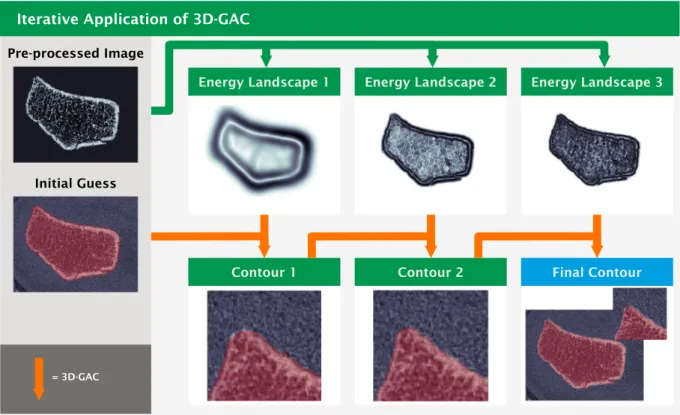
Fig. 2. Iterative approximation of the final contour via multiple 3D-GAC applications. The pre-processed images (top left and Fig. 1) is converted to an energy landscape using Gaussian blurring and computing the gradient to detect edges. Per iteration the blurring is reduced (top left to right) to allow for an increased amount of detail to be picked up by the 3D GAC per iteration. For the first iteration of 3D GAC the initial guess (bottom left and from Fig. 1) is used. Successive iterations then use the output of the previous iteration of the 3D GAC algorithm as the new initial guess (bottom).
number (Tb.N), trabecular thickness (Tb.Th), trabecular separation (Tb.
Sp), cortical perimeter (Ct.Pm), cortical thickness (Ct.Th), and intra- cortical porosity (Ct.Po) were computed for this study. The default setup uses outer contours generated by the approach of Buie et al. as input [13]. However, the standard patient evaluation pipeline also ac- cepts alternative outer contours as input. Outer contours generated from our novel 3D-GAC method were used as input to the standard patient evaluations and the resultant morphometrics were compared to those of the manufacturer’s default pipeline.
2.6. Study design
To assess the quality of the generated contours, we compared them to the respective gold standard for two different datasets (fractured and intact distal radii).
2.6.1. Fractured radii: comparison of the 3D-GAC approach to hand-drawn contours
The 3D-GAC method was run for all fracture images. Contours were visually categorized as acceptable, mistakenly including parts of the ulna, having obvious missing parts, or having both of these issues. Only images categorized as acceptable were used for additional quantitative analysis steps. Agreement between hand-drawn contour operators was assessed by computing the Dice score between their respective 2D contours for each image. The Dice score, similar to a percent agreement, quantifies differences between the contours with values ranging from zero to one. Zero indicates no overlap while one indicates a perfect match. Additionally, the distance transform of the area between the edges of 2D contours between operators was computed. Accuracy of the 3D-GAC approach was determined by taking the median Dice score between the 3D-GAC and the three hand-drawn 2D contours for each of the slices per image. The mean error ±standard deviation, calculated as percent difference in contour area, between the 3D-GAC and the hand- drawn contours was computed for each operator. Furthermore, all hand-drawn 2D contours created by the three operators were combined to yield a smallest and largest contour. The voxels between these two contours describes an area of uncertainty for the hand-drawn contours.
Voxels in the smallest hand-drawn 2D contour but not in the automatic one and voxels in the 3D-GAC contour but not in the largest hand-drawn 2D contour were extracted and a distance transform was applied as a measure for deviations of the 3D-GAC contours from the hand-drawn 2D ones. The automated default manufacturer pipeline was also run on all fracture images to generate outer contours and categorisation as for the 3D-GAC contours was performed.
2.6.2. Intact radii: Comparison of the 3D-GAC and Manufacturer’s approach
The 3D-GAC approach and the default manufacturer pipeline were run on all 73 intact radii (Fig. S1). Contours of both approaches were visually assessed and categorized as described previously for the frac- tured radii. For each patient, one image for which both approaches were successful was randomly chosen for further analysis. Accuracy of the 3D- GAC method was assessed by computing the Dice score between each contour of the 3D-GAC method and the respective contour of the man- ufacturer’s method. Additionally, the distance transform of the volume between the surfaces of both approaches was computed as another measure of how much the two methods deviated from each other.
Reproducibility was determined by computing the Dice score of each follow-up image with the baseline image for each patient. Morphomet- rics were computed to assess how strongly the computation of standard morphometric indices is influenced by the choice of outer contour.
2.7. Statistics
Bland-Altman plots were created in Python to assess systematic dif- ferences between hand-drawn and 3D-GAC contours. Additionally,
Bland-Altman plots were generated to assess systematic deviations be- tween morphometric indices generated from the default manufacturer and 3D-GAC contours. To allow visual comparison of the magnitudes of deviations between contour area and different morphometric parame- ters, all Bland-Altman plots had their y-axis scaled by 15% of the maximum x-value throughout this paper, which was the maximum value not leading to clipping of data. Robust linear models were fitted for Bland-Altman plots with Huber’s T for M estimation using the stats- models package in Python [30]. This package also provides two-sided Student’s t-tests for the linear models with zero slope and intercept of each Bland-Altman plot being the null-hypotheses, respectively. Here, the default significance level of α <0.05 was implemented.
Statistical significance for the comparison of morphometrics was performed using a paired Student’s t-test. Significance level was set to α
<0.05. Throughout the current work, significant differences are deno- ted using an asterisk (*).
3. Results
3.1. Fractured radii: comparison of the 3D-GAC approach to hand-drawn contours
From the 60 images, 20 were successfully contoured by both 3D-GAC and the default manufacturer pipeline. The default manufacturer pipe- line failed 40 times, while the 3D-GAC approach failed only for five images (Fig. 3a). The VGS for the failed contours of the manufacturer’s approach ranged from one to five, with 15% having VGS 1 (N =6), 50%
having VGS 2 (N =20), 22% having VGS 3 (N =9), 8% having VGS 4 (N
=3), and 5% having VGS 5 (N =2). For the five contours that only failed for the 3D-GAC approach, 60% had VGS 2 (N =3), 20% had VGS 3 (N = 1), and 20% had VGS 4 (N =1). Typically, the default manufacturer pipeline failed due to missing parts of the radius as a result of fracture gaps in the cortex (N =33), inclusion of parts of the ulna in the contour (N =2) or both (N =5). The 3D-GAC approach failed due to missing parts of the radius (N =2), inclusion of parts of the ulna in the contour (N =1), or inclusion of parts of the background in the contour (N =2).
Furthermore, the default manufacturer pipeline only showed a high success rate for images taken one-year post fracture (Fig. 3b), whereas the 3D-GAC worked similarly well for all time points. No specific rela- tionship was observed between failed 3D-GAC contours and individual patients, patient demographics, or VGS. The presence of the plaster cast in weeks 1 and 3 post-fracture did not result in any observable bias in the contour generated by the 3D-GAC approach (Fig. 6b,c), despite previous studies indicating plaster casts can have a considerable effect on HR- pQCT measurements [12,31]. The manufacturer’s approach performed similarly at 1, 3, 5, and 13 weeks post-fracture, indicating casting was not a contributing factor to the failed contour. Note that the default manufacturer pipeline has not been designed to handle images of frac- tured radii and therefore one could expect the unfavourable outcome.
Visually, contours matched the given bone structures well within the inter-operator variability (Fig. 4). The fracture images successfully contoured by the 3D-GAC approach (55 in total) were included in the validation (Fig. 3a). Agreement was found between the 3D-GAC approach and hand-drawn contours with a mean Dice score of 0.992
±0.005. This is within the range of inter-operator agreement: (operator 1 vs operator 2) 0.992 ±0.006, (operator 1 vs operator 3) 0.992 ± 0.006, and (operator 2 vs operator 3) 0.994 ±0.005. Evaluating the six appointments individually, Dice scores were high (>0.985), though some increase in the inter-quartile range of the Dice scores was observed between three and thirteen weeks post fracture (Fig. 3c). This coincided with a decrease in contouring success (Fig. 3b). For voxels of the 3D-GAC deviating from the area of uncertainty, 77% of these contour voxels were only one voxel away from at least one hand-drawn contour. This was within the inter-observer variability, as we observed (operator 1 vs operator 2) 56%, (operator 1 vs operator 3) 58%, and (operator 2 vs operator 3) 56% of deviations being less than one voxel away between
operators (Fig. 3d). Comparing the contour areas between the 3D-GAC method and the three operators, agreement was high with errors being: − 1.22 ±0.48%, − 0.48 ±0.5%, and − 0.29 ±0.49% for each operator, respectively. An underestimation of the total area was observed for the 3D-GAC contours (Fig. 5). This underestimation (Fig. 5d) is less than the measured difference comparing operator 1 to operator 3 (Fig. 5b): slope (− 0.003 vs − 0.011 (both significant)) and intercept (− 0.078 vs 0.087; both not significant).
3.2. Intact radii: comparison of the 3D-GAC and manufacturer’s approach
From the 438 images of intact radii, 341 were successfully contoured by both approaches. The default manufacturer pipeline failed for 85 images, the 3D-GAC approach failed for 3 images, and both approaches
failed for 9 images (Fig. 6a). The default manufacturer pipeline failed due to the inclusion of parts of the ulna into the radius contour (N =42), omission of large parts of the radius (N =37) (Fig. 7), inclusion of parts of the background in the contour (N =5), or inclusion of parts of the ulna into the radius contour while omitting large parts of the radius (N =10).
The 3D-GAC approach failed due to the inclusion of background (N =8), omission of large parts of the radius (N =1), omission of parts of the radius and inclusion of parts of the ulna in the contour (N =2), and all mentioned failure modes combined (N =1). The VGS for the failed contours of the manufacturer’s approach ranged from one to five, with 7% having VGS 1 (N =7), 15% having VGS 2 (N =14), 17% having VGS 3 (N =16), 32% having VGS 4 (N =30), and 29% having VGS 5 (N = 27). For the thirteen contours that only failed for the 3D-GAC approach, 7% had VGS 2 (N =1), 38% had VGS 4 (N =5), and 46% had VGS 5 (N
=6).
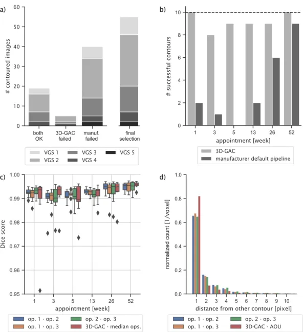
Fig. 3.Accuracy of the 3D-GAC approach vs hand-drawn contours for scans of fractured radii. a) Histogram of successful and failed contours for the 3D-GAC and the default manufacturer pipeline. The final bar shows the images selected for further analysis. Note that this pipeline was not designed to handle scans of fractured radii.
b) Histogram of successful contours for the two approaches per patient time-appointment. Dashed line indicates 100% success. c) Dice scores computed for all images between the hand-drawn slices of all operators (op) respectively. The corresponding slices of the 3D-GAC contours were also compared against the hand-drawn slices, respectively, and the average median Dice score is shown. d) Histogram of the distance, measured in pixels, of all voxels different between the 3D-GAC and the area of uncertainty (AOU) for the hand-drawn contours of each operator, respectively. The AOU is defined as the area between the contour obtained by only accepting voxels present in all hand-drawn contours and the contour obtained by accepting voxels present in at least one hand-drawn contour. Distances are displayed out to the 99th percentile (Range =1,21 pixels; pixel size =61 μm).
Of the 341 images successfully contoured by both approaches, one image per patient (N =72, one patient from the initial dataset was not successfully contoured by both approaches) with sufficient image quality (VGS of three or better) was randomly selected for comparative analysis. Overall agreement between the contours generated by both approaches was high with a mean Dice score of 0.996 ±0.001, with typical Dice score values for contours with missing parts of the radius being around 0.85. In total, 13 of the 19 patients from the reproduc- ibility study had their contralateral radius successfully contoured by both approaches for all timepoints; these images were used in the quantitative analysis. Reproducibility for the 3D-GAC approach was on the same level as the default manufacturer pipeline, wherein agreement with the baseline image for both methods and for all appointments was found (median Dice score >0.994 for all time-points) (Fig. 6b). For those voxels that were either part of the 3D-GAC contour and not part of the contour from the default manufacturer pipeline or vice versa, 91%
were at most one voxel away from the manufacturer’s contour (Fig. 6c).
Bland-Atman plots revealed agreement in morphometric indices with a slight thickness- and density-based bias in most cortical parameters and no bias in trabecular parameters (Fig. 8). Mean deviations were below 1% for all parameters except for Ct.Th (1.341%) (Table 1).
4. Discussion
4.1. Fractured radii: comparison of the 3D-GAC approach to hand-drawn contours
One of the main aims of the present study was to develop a fully
automatic outer contouring approach for HR-pQCT images of distal radius fractures. An image processing pipeline using a combination of adaptive histogram equalization, watershed segmentation, iterative Gaussian blurred energy landscapes, and 3D-GAC was established such that 55 out of 60 images were automatically contoured successfully. In our hand-contoured reference dataset, we observed clear inter-operator variability, which is a known issue of hand-contouring bone [32]. On average, the automatically generated contours by the 3D-GAC algorithm agreed well with operators. Interestingly, both hand-drawn and 3D-GAC contours had slightly larger inter-quartile ranges for appointments 2 and 3, likely as a result of the formation of a callus in this time period and the resulting low mineralization of background voxels visible in the HR- pQCT images. This makes it harder for both operators and the algo- rithm to decide on the correct contour. Given that no systematic de- viations were detected between operators and the 3D-GAC approach and that deviations from individual operators were within the range of inter- operator variability (Fig. 5), the 3D-GAC contouring approach devel- oped in this study provides accurate contours for HR-pQCT images of fractured distal radii compared to the gold standard.
As a point of reference, the default manufacturer’s pipeline was used to generate outer contours of the fractured images. The default manu- facturer pipeline only reliably contoured HR-pQCT images taken one- year post fracture (Fig. 3b). As this pipeline was not designed to work with images of impaired cortices, this might indicate structural weak- nesses in the cortex of the healing radii even 6 months post fracture. This observation is in agreement with recent findings suggesting that fracture repair is a long-term process which might take as long as two years [10].
op. 1
op. 1
op. 1 vs op. 2
op. 1 vs op. 3
op. 2 vs op. 3
op. 2 op. 3
op. 2 op. 3
hand-drawn contours
hand-drawn vs 3D-GAC
hand-drawn vs hand-drawn
only selected by upper operator
agreement only selected by
lower operator
3D-GAC
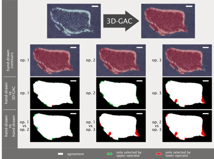
Fig. 4. Visual comparison of hand-drawn contours (by three different operators (op)) and 3D geodesic active contour (3D-GAC) generated contours for a repre- sentative challenging slice from one week post-fracture. Visual differences between the 3D-GAC and hand-drawn contours are similar to those between hand-drawn contours of different operators. Scale bar is 2 mm.
4.2. Intact radii: comparison of the 3D-GAC and manufacturer’s approach
The second aim of the present study was to evaluate the robustness of the 3D-GAC contours against the default manufacturer pipeline by comparing the resultant morphometrics. Notably, the failure rate of the automated manufacturer default pipeline was much higher than that of the 3D-GAC approach for the HR-pQCT images of the intact radii (94 vs 12 failed contours, respectively). This may be a result of the patient cohort used in the present study since fracture patients have been shown to have inherently poorer bone quality than standard populations [33].
One of the major reasons for failure of the default manufacturer pipeline was the inclusion of the ulna into the outer contour of the radius, which is a known issue of this approach that is implementation dependent [13]. The second reason for failure was having obvious missing parts, which appeared to happen when the cortex had very thin or low-density structures (Fig. 7). The authors would like to emphasise that these failures of the default manufacturer pipeline can be, and often are,
overcome by generating hand-drawn contours using a built-in tool of the manufacturer’s software. However, as noted previously, the cost in person-hours of such a solution is prohibitive in large patient cohort studies. An automated solution for this issue was proposed by Buie and co-workers [13]; here, they increased the number of dilation steps of the manufacturer’s pipeline but noted that this often lead to unwanted smoothing of the contour [13]. Moreover, defining per-image numbers of dilation steps would reduce the degree of automation drastically. Both approaches were affected by image quality, as expected. However, the 3D-GAC approach only failed for one image with sufficient image quality to be considered for inclusion in HR-pQCT studies [8,32,34].
Trabecular morphometric indices generated using the successful 3D- GAC contours agreed well with those generated using the default manufacturer pipeline with deviations well below the precision error of these indices [35]. Interestingly, for the cortical parameters, accuracy was slightly worse for Ct.Th generated using the 3D-GAC approach, showing deviations of 1–2%, while accuracy for Ct.Po was unaffected by the contouring approach. Note that the differences in Ct.Th were still Fig. 5.Bland-Altman plots of the mean contour area per image. a) Comparing operator 1 (op. 1) to operator 2 (op. 2). b) Comparing operator 1 to operator 3 (op. 3).
c) Comparing operator 2 to operator 3. d) Comparing the automatic 3D-GAC contours with the median (computed per slice) of all three operators. Area computed with the 3D-GAC approach agrees within the observable inter-operator variability with the area computed from hand-draw contours. Dashed lines indicate ±1.96 standard deviations of the mean. Regression parameters are presented above each plot with slope and intercept parameters statistically significantly different from zero being indicated by (*, P <0.05).
Fig. 6. Accuracy and reproducibility of the 3D-GAC vs the default manufacturer pipeline (DMP). a) Histogram of successful and failed contours for the 3D-GAC and the DMP with indicated image quality. The final bar shows the images selected for the reproducibility analysis. b) Dice scores of contours of all time points relative to the initial scan for both approaches show the reproducibility of each method. c) Histogram of the distance, measured in pixels, of all voxels different between the 3D- GAC and the DMP contour from the respective DMP contour. Distances are displayed out to the 99th percentile (Range =1, 9 pixels; pixel size =61 μm).
3D-GAC
default manufact.
pipeline
missing parts of radius
partial inclusion of ulna
missing parts of radius &
partial inclusion of ulna low visual grading score Fig. 7.Examples of failure modes when contouring distal radii. Contours from the 3D-GAC and the default manufacturer pipeline are compared for four challenging contouring cases: A thin cortex leading to missing parts of the radius, the ulna (partly being visible on the right) being close to the radius (bone on the left) and hence being included in the contour, the combination of the previous two, and a low visual grading score. Only the 3D-GAC approach manages to generate visually correct contours in most cases. Scale bar is 2 mm.
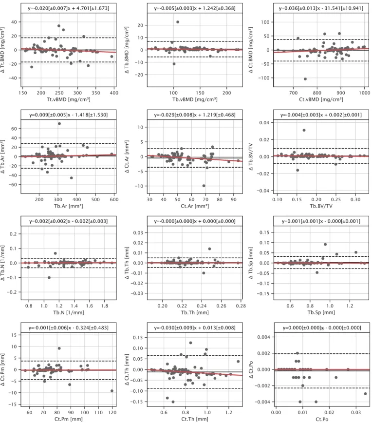
Fig. 8. Bland-Altman plots of morphometric indices characterize potential differences in 3D-GAC and contours from the default manufacturer pipeline. Robust linear model fits are shown in red. Regression parameters are presented above each plot with slope and intercept parameters statistically significantly different from zero being indicated by (*, P <0.05). Indices are total volumetric bone mineral density (Tt.BMD), trabecular volumetric bone mineral density (Tb.BMD), cortical volumetric bone mineral density (Ct.BMD), trabecular area (Tb.Ar), cortical area (Ct.Ar), trabecular bone volume fraction (Tb.BV/TV), trabecular number (Tb.N), trabecular thickness (Tb.Th), trabecular separation (Tb.Sp), cortical perimeter (Ct.Pm), cortical thickness (Ct.Th), intra-cortical porosity (Ct.Po). (For interpretation of the references to colour in this figure legend, the reader is referred to the web version of this article.)
less than 1 voxel in thickness and thus at the accuracy limit of the device (Fig. 6). Furthermore, differences in Ct.Th were at the reproducibility limit of the standard patient evaluation (1.3–3.9% dependent on subject age) [36] and were still below differences observed between patient groups from the literature, e.g. healthy and osteopenic women (12.8%) [37]. The lack of sensitivity of Ct.Po to the contouring approach can be attributed to the nature of the measurement. Pores that intersect the periosteal or endocortical surfaces, most likely to be affected by the contour, are not captured by the threshold-based approach implemented in the gold standard patient evaluation [38]. Given the improved success rate and accurate determination of morphometric indices, the 3D-GAC approach showed an overall improvement in robustness compared to the current gold standard.
Lastly, the present study aimed to determine the reproducibility of the 3D-GAC approach using sequential image scans of the intact radii taken over the course of a year. Here, agreement with the baseline contour was found to be high for all time points (Dice scores >0.994).
Again, deviations in Ct.Th were highest, but well within the reproduc- ibility limit of the standard patient evaluation.
Given the improved robustness and sufficient reproducibility, the 3D-GAC approach appears to be a viable option for clinical studies of both fractured and non-fractured radii.
4.3. Limitations
This study is not without limitations. The repeat scans of the contralateral site were spaced over a year, and thus may include vari- ations in bone due to natural remodelling. Additional reproducibility scans could not be taken for these patients due to radiation concerns.
Future studies should include follow-up scans at protracted intervals to assess how sensitive the 3D-GAC approach is to local and global remodelling. Due to the large structural changes happening during fracture repair, the images of the fracture site could not be regarded as repeat scans. Therefore, no direct assessment of reproducibility was possible for images of fractured radii. However, the high accuracy observed between the hand-drawn and 3D-GAC contours of the frac- tured images indicates a high level of reproducibility. Another limitation is the low number of hand-drawn contour slices (1800 total, 1650 used in the analysis, Fig. S1) generated to use as reference. While time was a limiting factor (operators reporting to take roughly 1–2 min per slice) for creating more hand-drawn contours, we compensated by including im- ages of the intact contralateral site to cover a large variety of bone morphologies in our assessment of the 3D-GAC robustness and
repeatability. These images of the intact radius provided a means to benchmark the 3D-GAC approach against existing automatic approaches for intact radii. Note that the 3D-GAC contours were generated only proximal to the lunate fossa, excluding the articulating surface.
Although this limits the range over which the 3D-GAC approach can be applied, the morphometric analysis of the standard patient evaluation has only been developed for that region; as such, this region remains the most relevant for clinical studies. While images with VGS 4 and 5 are typically excluded in clinical studies, 7 of our 55 fracture images included in the quantitative analysis had VGS of 4 or 5. A recent study explored the use of poor quality images (VGS 4) in finite element analysis of radius and tibia HR-pQCT scans [39]. Therefore, we opted to include these in the assessment of the 3D-GAC algorithm performance.
Lastly, no hand-corrected contours were generated for intact radii to estimate the bias introduced by the automated manufacturer and 3D- GAC protocols. However, recent studies have already done this for the gold standard [40] and, given the good agreement of the 3D-GAC approach with the gold standard, the requirement for minor manual corrections should be on a similar level.
5. Conclusion
Our proposed 3D-GAC algorithm provides a unified pipeline for generating outer contours from HR-pQCT images of distal radii, including both fractured and intact bones. Importantly, our method automatically contours radii both accurately and reproducibly, while showing robustness when dealing with a wide variety of cortex struc- tures. This will facilitate future clinical studies using large patient co- horts to support the development of improved treatment protocols of radius fractures.
Supplementary data to this article can be found online at https://doi.
org/10.1016/j.bone.2021.115930.
CRediT authorship contribution statement
Nicholas Ohs: Conceptualization, Methodology, Software, Formal Analysis, Validation, Writing – Original Draft, Writing – Review, Editing.
Caitlyn J. Collins: Conceptualization, Investigation, Data Curation, Validation, Writing – Original Draft, Writing – Review, Editing.
Duncan C. Tourolle: Conceptualization, Investigation, Resources, Writing – Original Draft.
Penny R. Atkins: Conceptualization, Investigation, Data Curation, Writing – Original Draft, Writing – Review, Editing.
Bryant Schroeder: Investigation, Data Curation.
Michael Blauth: Funding acquisition, Writing – Review, Editing.
Patrik Christen: Funding acquisition, Supervision, Writing – Re- view, Editing.
Ralph Müller: Funding acquisition, Supervision, Writing – Review, Editing.
Declaration of competing interest
Dr. Michael Blauth consults for the Clinical Medical Department of DePuy Sythes in Zuchwil, Switzerland. The remaining authors declare that they have no known competing financial interests or personal re- lationships that could have appeared to influence the work reported in this paper.
Acknowledgements
The authors acknowledge the Swiss National Science Foundation (320030L_170205), the European Union’s Horizon 2020 Research and Innovation Programme under the Marie Skłodowska-Curie grant (agreement 841316), and the ETH Postdoctoral Fellowship for financial support. The funders had no role in study design, data collection and Table 1
Deviations of the bone morphometrics derived using 3D-GAC based contours compared to the manufacturer’s default pipeline.
Morphometric Index Deviation from Gold Standard
Tt.BMD 0.190 ±3.668%
Tb.BMD 0.662 ±3.226%
Ct.BMD −0.131 ±2.437%
Tb.Ar 0.510 ±4.920%
Ct.Ar −0.710* ±2.530%
Tb.BV/TV 0.540 ±2.830%
Tb.N −0.093 ±1.497%
Tb.Th 0.147 ±1.017%
Tb.Sp 0.181 ±1.625%
Ct.Pm −0.333 ±2.402%
Ct.Th −1.341* ±4.911%
Ct.Po −1.215 ±8.788%
Morphometric Indices: total volumetric bone mineral density (Tt.BMD), trabecular volumetric bone mineral density (Tb.BMD), cortical volumetric bone mineral density (Ct.BMD), trabecular area (Tb.Ar), cortical area (Ct.
Ar), trabecular bone volume fraction (Tb.BV/TV), trabecular number (Tb.N), trabecular thickness (Tb.Th), trabecular separation (Tb.Sp), cortical perim- eter (Ct.Pm), cortical thickness (Ct.Th), intra-cortical porosity (Ct.Po).
*Indicates significant deviation (P <0.05).
analysis, decision to publish, or preparation of the manuscript.
References
[1] O. Johnell, J.A. Kanis, An estimate of the worldwide prevalence and disability associated with osteoporotic fractures, Osteoporos. Int. 17 (2006) 1726–1733, https://doi.org/10.1007/s00198-006-0172-4.
[2] C.M. Court-Brown, B. Caesar, Epidemiology of adult fractures: a review, Injury. 37 (2006) 691–697, https://doi.org/10.1016/j.injury.2006.04.130.
[3] C.Y. Ng, M.M. McQueen, What are the radiological predictors of functional outcome following fractures of the distal radius? J. Bone Jt. Surg. - Ser. B. 93 (B) (2011) 145–150, https://doi.org/10.1302/0301-620X.93B2.25631.
[4] A.J. Burghardt, G.J. Kazakia, M. Sode, A.E. De Papp, T.M. Link, S. Majumdar, A longitudinal HR-pQCT study of alendronate treatment in postmenopausal women with low bone density: relations among density, cortical and trabecular microarchitecture, biomechanics, and bone turnover, J. Bone Miner. Res. 25 (2010) 2558–2571, https://doi.org/10.1002/jbmr.157.
[5] V.V. Shanbhogue, R.K. Støving, K.H. Frederiksen, S. Hanson, K. Brixen, J. Gram, N.
R. Jørgensen, S. Hansen, Bone structural changes after gastric bypass surgery evaluated by HR-pQCT: a two-year longitudinal study, Eur. J. Endocrinol. 176 (2017) 685–693, https://doi.org/10.1530/EJE-17-0014.
[6] L.A. Burt, D.A. Hanley, S.K. Boyd, Cross-sectional versus longitudinal change in a prospective HR-pQCT study, J. Bone Miner. Res. 32 (2017) 1505–1513, https://
doi.org/10.1002/jbmr.3129.
[7] R. Ellouz, R. Chapurlat, B. van Rietbergen, P. Christen, J.B. Pialat, S. Boutroy, Challenges in longitudinal measurements with HR-pQCT: evaluation of a 3D registration method to improve bone microarchitecture and strength measurement reproducibility, Bone. 63 (2014) 147–157, https://doi.org/10.1016/j.
bone.2014.03.001.
[8] K.K. Nishiyama, Y. Pauchard, L.E. Nikkel, S. Iyer, C. Zhang, D.J. McMahon, D. Cohen, S.K. Boyd, E. Shane, T.L. Nickolas, Longitudinal HR-pQCT and image registration detects endocortical bone loss in kidney transplantation patients, J. Bone Miner. Res. 30 (2015) 456–463, https://doi.org/10.1002/jbmr.2358.
[9] J.J.A. De Jong, P.C. Willems, J.J. Arts, S.G.P. Bours, P.R.G. Brink, T.A.C.M. van Geel, M. Poeze, P.P. Geusens, B. van Rietbergen, J.P.W. van den Bergh, Assessment of the healing process in distal radius fractures by high resolution peripheral quantitative computed tomography, Bone. 64 (2014) 65–74, https://doi.org/
10.1016/j.bone.2014.03.043.
[10] J.J. de Jong, F.L. Heyer, J.J.C. Arts, M. Poeze, A.P. Keszei, P.C. Willems, B. van Rietbergen, P.P. Geusens, J.P. van den Bergh, Fracture repair in the distal radius in postmenopausal women: a follow-up 2 years Postfracture using HRpQCT, J. Bone Miner. Res. 31 (2016) 1114–1122, https://doi.org/10.1002/jbmr.2766.
[11] J.J.A. De Jong, P. Christen, R.M. Plett, R. Chapurlat, P.P. Geusens, J.P.W. Van Den Bergh, R. Müller, B. Van Rietbergen, Feasibility of rigid 3D image registration of high-resolution peripheral quantitative computed tomography images of healing distal radius fractures, PLoS One. 12 (2017), https://doi.org/10.1371/journal.
pone.0179413.
[12] D.E. Whittier, S.L. Manske, S.K. Boyd, P.S. Schneider, The correction of systematic error due to plaster and fiberglass casts on HR-pQCT bone parameters measured in vivo at the distal radius, J. Clin. Densitom. 22 (2019) 401–408, https://doi.org/
10.1016/j.jocd.2018.11.005.
[13] H.R. Buie, G.M. Campbell, R.J. Klinck, J.A. MacNeil, S.K. Boyd, Automatic segmentation of cortical and trabecular compartments based on a dual threshold technique for in vivo micro-CT bone analysis, Bone. 41 (2007) 505–515, https://
doi.org/10.1016/j.bone.2007.07.007.
[14] A.J. Burghardt, G.J. Kazakia, S. Majumdar, A local adaptive threshold strategy for high resolution peripheral quantitative computed tomography of trabecular bone, Ann. Biomed. Eng. 35 (2007) 1678–1686, https://doi.org/10.1007/s10439-007- 9344-4.
[15] A.J. Burghardt, H.R. Buie, A. Laib, S. Majumdar, S.K. Boyd, Reproducibility of direct quantitative measures of cortical bone microarchitecture of the distal radius and tibia by HR-pQCT, Bone. 47 (2010) 519–528, https://doi.org/10.1016/j.
bone.2010.05.034.
[16] R. Zebaze, A. Ghasem-Zadeh, A. Mbala, E. Seeman, A new method of segmentation of compact-appearing, transitional and trabecular compartments and
quantification of cortical porosity from high resolution peripheral quantitative computed tomographic images, Bone. 54 (2013) 8–20, https://doi.org/10.1016/j.
bone.2013.01.007.
[17] M. Kass, A. Witkin, D. Terzopoulos, Snakes: active contour models, Int. J. Comput.
Vis. 1 (1988) 321–331, https://doi.org/10.1007/BF00133570.
[18] M. Hafri, H. Toumi, S. Boutroy, R.D. Chapurlat, E. Lespessailles, R. Jennane, Fuzzy energy based active contours model for HR-PQCT cortical bone segmentation, in:
2016 IEEE Int. Conf. Image Process., IEEE, 2016, pp. 4334–4338, https://doi.org/
10.1109/ICIP.2016.7533178.
[19] M. Hafri, R. Jennane, E. Lespessailles, H. Toumi, Dual active contours model for HR-pQCT cortical bone segmentation, in: 2016 23rd Int. Conf. Pattern Recognit., IEEE, 2016, pp. 2270–2275, https://doi.org/10.1109/ICPR.2016.7899974.
[20] V. Caselles, R. Kimmel, G. Sapiro, Geodesic active contours, Int. J. Comput. Vis. 22 (1997) 61–79, https://doi.org/10.1023/A:1007979827043.
[21] P. Marquez-Neila, L. Baumela, L. Alvarez, A morphological approach to curvature- based evolution of curves and surfaces, IEEE Trans. Pattern Anal. Mach. Intell. 36 (2014) 2–17, https://doi.org/10.1109/TPAMI.2013.106.
[22] J.B. Pialat, A.J. Burghardt, M. Sode, T.M. Link, S. Majumdar, Visual grading of motion induced image degradation in high resolution peripheral computed tomography: impact of image quality on measures of bone density and micro- architecture, Bone. 50 (2012) 111–118, https://doi.org/10.1016/j.
bone.2011.10.003.
[23] J.L. Marsh, T.F. Slongo, J. Agel, J.S. Broderick, W. Creevey, T.A. DeCoster, L. Prokuski, M.S. Sirkin, B. Ziran, B. Henley, L. Audig´e, Fracture and Dislocation Classification Compendium, Orthopaedic trauma association classification, database and outcomes committee, J. Orthop. Trauma 21 (2007) (2007). https://jo urnals.lww.com/jorthotrauma/Fulltext/2007/11101/Fracture_and_Dislocatio n_Classification_Compendium.1.aspx.
[24] P. Th´evenaz, U.E. Ruttimann, M. Unser, A pyramid approach to subpixel registration based on intensity, IEEE Trans. Image Process. 7 (1998) 27–41, https://doi.org/10.1109/83.650848.
[25] The HDF, Group, Hierarchical Data Format, Version 5. http://www.hdfgroup.
org/HDF5/, 2020.
[26] Python Software Foundation, Python Language Reference, Version 3.7. http s://www.python.org, 2020.
[27] S. Van Der Walt, J.L. Sch¨onberger, J. Nunez-Iglesias, F. Boulogne, J.D. Warner, N. Yager, E. Gouillart, T. Yu, Scikit-image: image processing in python, PeerJ. 2014 (2014) 1–18, https://doi.org/10.7717/peerj.453.
[28] S. Van Der Walt, S.C. Colbert, G. Varoquaux, The NumPy array: a structure for efficient numerical computation, Comput. Sci. Eng. 13 (2011) 22–30, https://doi.
org/10.1109/MCSE.2011.37.
[29] P. Virtanen, R. Gommers, T.E. Oliphant, M. Haberland, T. Reddy, D. Cournapeau, E. Burovski, P. Peterson, W. Weckesser, J. Bright, S.J. van der Walt, M. Brett, J. Wilson, K.J. Millman, N. Mayorov, A.R.J. Nelson, E. Jones, R. Kern, E. Larson, C. Carey, ˙I. Polat, Y. Feng, E.W. Moore, J. VanderPlas, D. Laxalde, J. Perktold, R. Cimrman, I. Henriksen, E.A. Quintero, C.R. Harris, A.M. Archibald, A.H. Ribeiro, F. Pedregosa, P. van Mulbregt, S. 1. 0 Contributors, SciPy 1.0–Fundamental Algorithms for Scientific Computing in Python, 2019, pp. 1–22. http://arxiv.
org/abs/1907.10121.
[30] S. Seabold, J. Perktold, Statsmodels: econometric and statistical modeling with python, in: 9th Python Sci. Conf., 2010.
[31] J.J.A. De Jong, J.J. Arts, U. Meyer, P.C. Willems, P.P. Geusens, J.P.W. Van Den Bergh, B. Van Rietbergen, Effect of a cast on short-term reproducibility and bone parameters obtained from HR-pQCT measurements at the distal end of the radius, J. Bone Jt. Surg. - Am. Vol. 98 (2016) 356–362, https://doi.org/10.2106/JBJS.
O.00127.
[32] E.A.C. de Waard, C. Sarodnik, A. Pennings, J.J.A. de Jong, H.H.C.M. Savelberg, T.
A. van Geel, C.J. van der Kallen, C.D.A. Stehouwer, M.T. Schram, N. Schaper, P.
C. Dagnelie, P.P.M.M. Geusens, A. Koster, B. van Rietbergen, J.P.W. van den Bergh, Reliability of HR-pQCT Derived Cortical Bone Structural Parameters When Using Uncorrected Instead of Corrected Automatically Generated Endocortical Contours in a Cross-Sectional Study: The Maastricht Study, Calcif. Tissue Int. 103 (2018) 252–265, https://doi.org/10.1007/s00223-018-0416-2.
[33] H. Mallmin, S. Ljunghall, Distal radius fracture is an early sign of general osteoporosis: bone mass measurements in a population-based study, Osteoporos.
Int. 4 (1994) 357–361, https://doi.org/10.1007/BF01622198.
[34] S.L. Manske, E.M. Davison, L.A. Burt, D.A. Raymond, S.K. Boyd, The estimation of second-generation HR-pQCT from first-generation HR-pQCT using in vivo cross- calibration, J. Bone Miner. Res. 32 (2017) 1514–1524, https://doi.org/10.1002/
jbmr.3128.
[35] T.L. Mueller, M. Stauber, T. Kohler, F. Eckstein, R. Müller, G.H. van Lenthe, Non- invasive bone competence analysis by high-resolution pQCT: an in vitro reproducibility study on structural and mechanical properties at the human radius, Bone. 44 (2009) 364–371, https://doi.org/10.1016/j.bone.2008.10.045.
[36] A.J. Burghardt, H.R. Buie, A. Laib, S. Majumdar, S.K. Boyd, Reproducibility of direct quantitative measures of cortical bone microarchitecture of the distal radius and tibia by HR-pQCT, Bone. 47 (2010) 519–528, https://doi.org/10.1016/j.
bone.2010.05.034.
[37] K.K. Nishiyama, H.M. Macdonald, H.R. Buie, D.A. Hanley, S.K. Boyd,
Postmenopausal women with osteopenia have higher cortical porosity and thinner cortices at the distal radius and tibia than women with normal aBMD: an in vivo HR-pQCT study, J. Bone Miner. Res. 25 (2010) 882–890, https://doi.org/10.1359/
jbmr.091020.
[38] D.E. Whittier, S.K. Boyd, A.J. Burghardt, J. Paccou, A. Ghasem-Zadeh, R. Chapurlat, K. Engelke, M.L. Bouxsein, Guidelines for the assessment of bone density and microarchitecture in vivo using high-resolution peripheral quantitative computed tomography, Osteoporos. Int. 31 (2020) 1607–1627, https://doi.org/
10.1007/s00198-020-05438-5.
[39] D. Schenk, A. Mathis, K. Lippuner, P. Zysset, In vivo repeatability of homogenized finite element analysis based on multiple HR-pQCT sections for assessment of distal radius and tibia strength, Bone. 141 (2020) 115575, https://doi.org/10.1016/j.
bone.2020.115575.
[40] D.E. Whittier, A.N. Mudryk, I.D. Vandergaag, L.A. Burt, S.K. Boyd, Optimizing HR- pQCT workflow: a comparison of bias and precision error for quantitative bone analysis, Osteoporos. Int. 31 (2020) 567–576, https://doi.org/10.1007/s00198- 019-05214-0.