Systematic Survey of the Correlation between Northern HECR Events and SDSS Galaxies

arXiv:0910.2765v2 [astro-ph.HE] 14 Oct 2011

Systematic Survey of the Correlation between Northern HECR Events and SDSS Galaxies

Hajime Takami

, Takahiro Nishimichi

, and Katsuhiko Sato

1

Max Planck Institute for Physics, F¨ ohringer Ring 6, 80805 Munich, Germany

2

Institute for the Physics and Mathematics of the Universe, the University of Tokyo, 5-1-5, Kashiwanoha, Kashiwa, Chiba 277-8583, Japan

3

National Institutes of Natural Sciences, 4-3-13, Toranomon, Minato-ku, 105-0001 Tokyo, Japan

We investigated the spatial correlation between the arrival directions of the highest en- ergy cosmic rays (HECRs) detected by the Akeno Giant Air Shower Array (AGASA) with energies above 4 × 10

eV and the positions of galaxies observed by the Sloan Digital Sky Survey (SDSS) within z = 0.024. We systematically tested the dependence of the correla- tion on the redshift ranges and properties of the galaxies, i.e., absolute luminosity, color, and morphology, to understand where HECR sources are and what objects are HECR sources.

In the systematic survey, we found potential signals of the positive correlation at small an- gular scale (< 10

) with the (non-penalized) chance probability less than 5% in intermediate redshift ranges. Then, we estimated penalized probabilities to compensate the trial effects of angular scan, and found that the strongest correlation is produced by early-type galaxies in 0.012 ≤ z < 0.018 at 90% C.L. The possible origin of HECRs which correlating galaxies imply is also discussed.

Subject Index: 411

§ 1. Introduction

The origin of the highest energy cosmic rays (HECRs) is an intriguing problem in astrophysics. It is widely believed that HECRs are of extragalactic origin because they cannot be confined in the Galaxy by a Galactic magnetic field (GMF) and their arrival direction distribution does not correlate with Galactic plane. Plausible source candidates of HECRs ever discussed are γ -ray bursts (GRBs),

radio- loud active galactic nuclei (AGN),

radio-quiet AGN,

magnetars,

and clusters of galaxies.

The sources of cosmic rays with ∼ 10

eV detected at the Earth are limited to objects with distances less than 100 Mpc because of in- teractions of HECRs with cosmic microwave background (CMB) photons, so-called Greisen-Zatsepin-Kuz’min (GZK) mechanism.

Thus, it is expected that the arrival directions of HECRs correlate with the directions of their sources if the de- flections of HECR trajectories by a GMF and intergalactic magnetic fields (IGMFs) are not large. The Akeno Giant Air Shower Array (AGASA) reported anisotropy in the arrival distribution of HECRs at small angular scale, which is comparable with the accuracy of the determination of the arrival directions of HECRs.

This anisotropy has been thought to be appearance of nearby astrophysical sources, but HECR sources have not been clear yet.

Important progress was brought in by the Pierre Auger Observatory (PAO).

The PAO reported a correlation between the arrival directions of 27 cosmic rays

typeset using PTP TEX.cls hVer.0.9i

with energies above ∼ 5.7 × 10

eV and the positions of galaxies listed in the 12th Veron-Cetty and Veron (VC) catalog

with z ≤ 0.018 within the angular scale of

∼ 3.1

.

Although the VC catalog is for AGN, the original argument of the PAO conservatively claimed that the distribution of cosmic ray sources is correlated with matter distribution in local Universe involving AGN because the spatial distribution of the underlying matter density correlates with that of AGN, i.e., the AGN listed in the VC catalog are just tracers of the matter distribution.

Several groups have also analyzed the PAO data by using catalogs of different astrophysical objects: X- ray selected AGN,

HI-selected galaxies,

and infrared-selected galaxies,

and they all reported significant correlations. Thus, the PAO data indicates that HECR sources are distributed to being comparable with the matter distribution in local Universe. Although the number of detected events is increasing after the first publication, the significance is fluctuating between 2σ and 3σ.

The PAO can observe only the southern sky because it is located in Argentina.

Is the correlation feature universal even in the northern sky? There are two reasons why the answer of this question is not trivial. The first reason is the structure of a GMF. Although its impact depends on GMF models, several models indicate that the typical deflection angles of HECR trajectories in Galactic space is different between in the northern sky and in the southern sky.

The second reason is the results of composition measurements. The measurements of hX

i and its fluctuation by the PAO indicate heavy nuclei dominated composition at the highest energies,

while those by the High Resolution Fly’s Eye (HiRes), which is a fluorescence detector in the northern hemisphere, imply proton-dominated composition.

Although this is a controversial issue, if this difference is intrinsic, HECRs detected in the northern sky experience smaller deflections and could produce stronger correlation.

The correlation between HECRs and the matter distribution in the northern sky has been discussed. Refs. 31) and 32) reported the correlation of HECRs with the supergalactic plane. We also examined the correlation of the AGASA data with galaxies listed in Infrared Astronomical Satellite Point Source Redshift Survey (IRAS PSCz) catalog,

but did not find significantly positive correlation.

Recently, the HiRes reported no significant correlation based on the same analysis as the PAO using its own data.

The HiRes also tested correlation between its data and galaxies observed by 2 Micron All-Sky Redshift Survey (2MASS),

but they reported no significant correlation at 95% C.L..

In this study, we test the correlation between the AGASA events as a represen-

tative of HECR event sets detected in the northern sky and galaxies observed by the

Sloan Digital Sky Survey (SDSS).

The SDSS observes even fainter galaxies down

to m

∼ 20.0, where m

is the r-band apparent magnitude of galaxies, and gives

us dense galaxy samples, which can well reflect galaxy distribution at small angular

scale even by using volume-limited samples. A SDSS sample of galaxies used in this

study has more than 10,000 galaxies within ∼ 100 Mpc (z = 0.024) after cuts for a

volume-limited sample (see Section 2.2) in spite of its small sky coverage (∼ 20% of

the entire sky). For comparison, note that the 2MASS sample used by the HiRes

has 15,508 galaxies in the HiRes field of view (about a half of the whole sky) within

250 Mpc. In addition, the completeness of the observed sky is well studied, which

enables us to estimate the geometry of the galaxy survey precisely.

Recent studies on the correlation between HECRs and galaxies in astronomical catalogue have regarded the galaxies as representatives of the matter distribution in local Universe. However, the statistical properties of the distribution of galaxies are, in general, different among the types of galaxies, which has been well studied in the field of cosmology. This can be easily understood when rare objects such as strong radio galaxies are considered. This viewpoint is useful to understand HECR sources and many works have been dedicated to test the correlation between HECRs and source candidates, i.e., different types of galaxies. Refs. 37) and 38) studied the correlation with infrared galaxies using the IRAS PSCz catalog of galaxies

and discussed the possibility that the AGASA events below ∼ 10

eV arrive from luminous infrared galaxies. The correlation of the AGASA and Yakutsk data with BL Lac objects was also suggested.

AGN in the Rossi X-ray Timing Ex- plorer (RXTE) catalog was tested, but do not correlate with HECRs significantly.

Ref. 43) performed a comprehensive study of the correlation with various classes of extragalactic objects and pointed out that BL Lac objects and unidentified gamma- ray sources might correlate with the AGASA and Yakutsk data.

Following this standpoint, we focus on the correlation with galaxies, not the underlying matter distribution. We examine the dependence of the correlation on the properties of galaxies systematically to investigate what objects correlate with HECRs. Since galaxies hosted by HECR sources have characteristic features, which depends on source population (discussed in Section 4), the dependence on the prop- erties of galaxies correlating with HECRs gives useful information on HECR sources.

Quantities attached to a SDSS catalog of galaxies allow to calculate useful astronom- ical quantities of galaxies, e.g., color and morphology of galaxies.

A volume-limited sample of galaxies lacks some information on darker galaxies than a cut criterion. Ref. 44) proposed a useful method to construct a flux reference map of HECRs with compensating this effect. In this method, weights are given to visible galaxies instead of galaxies invisible due to their darkness to correct selection effects by a flux limit. However, the weights does not consider the properties of invisible galaxies. Since we want to examine the dependence of the correlation on the properties of galaxies in this study, we analyze the HECR data by using volume- limited samples instead of this method. Thus, since we need dense galaxy samples to resolve galaxy distribution even at small angular scale, a SDSS catalog of galaxies is appropriate for this study, despite that about a half of the AGASA events does not overlap the field surveyed by the SDSS.

This paper is laid out as follows: the details of HECR events and galaxies

used for analysis, and a statistical method to test the correlation between them

are described in Section 2. In Section 3, the results of our statistical analysis are

presented. Firstly, we test the correlation of HECR events and galaxies in four

redshift ranges to investigate where HECR sources are in Section 3.1. Next, we

examine the dependence of the correlation on the properties of galaxies and search

for the potential signals of positive correlation in the following two sections. Then,

we compensate statistical penalties and estimate the true significance of the positive

correlation in Section 3.4. Section 4 is devoted to discuss the relation between HECR

source candidates and the properties of their host galaxies. Finally, we conclude this study in Section 5.

§ 2. Data Samples and Statistical Method 2.1. Sample of highest energy cosmic rays

As a sample of HECR events detected in the northern sky, the AGASA events listed in Ref. 45) are adopted. The AGASA event is the largest HECR sample detected in the northern sky in which the energy and arrival direction of each event are published. Although the total exposure of the HiRes is larger than that of the AGASA, the HiRes has not published the properties of each event. In addition, the AGASA is a ground array, and therefore its duty cycle is approximately 100%. This fact allows us to estimate the directional dependence of its aperture analytically.

The AGASA sample consists of 57 events with energies above 4× 10

eV. These events are distributed in the sky of −10

≤ δ ≤ 80

, where δ is the declination of the arrival direction of each cosmic ray. 8 events out of the 57 events have energies above 10

eV, which lead to the extension of cosmic ray spectrum beyond the predicted GZK cutoff.

The excess events over the GZK cutoff have sometimes been thought to originate from new physics beyond the standard model (see Ref. 47) for a review), but the HiRes and PAO have recently reported HECR spectra with a GZK-like feature,

which indicate astrophysical origin of HECRs. Although the reason of the excess events is still unclear, we assume that all the AGASA events are of astrophysical origin and use them in this paper.

2.2. Sample of galaxies

Volume-limited samples of galaxies used in this study are constructed from the 7th data release (DR7) of the SDSS,

especially large-scale structure subsam- ple named dr72bright0 sample of the New York University Value Added Catalog (NYU-VAGC).

This is a spectroscopic sample of galaxies with u,g,r,i,z-band (K-corrected) absolute magnitudes, r-band apparent magnitude m

, redshift, an indicator of the morphology, and information on the mask of the survey. These spectroscopic galaxies are selected by the conditions of 10.0 ≤ m

≤ 17.6 and 0.001 ≤ z ≤ 0.5. In fact, the upper bound of apparent magnitude of galaxies is less than 17.6 in a very small fraction of regions, but it is practically no problem to regard the upper bound as 17.6 because the fraction of such regions is less than 0.1%.

The flux limit m

= 17.6 restricts galaxies observed at each redshift, i.e., the maxi- mum r-band absolute magnitude M

of observed galaxies depends on their redshifts.

In order to avoid this dependence, we construct the samples of galaxies limited by

a constant M

within redshift which we are interested in, so-called volume-limited

samples. We focus on galaxies within ∼ 100 Mpc in this study, which corresponds

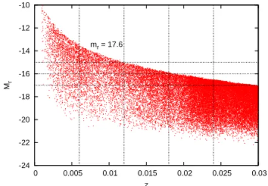
to z ∼ 0.024 in the standard ΛCDM cosmology. Fig. 1 plots all the galaxies within

z ≤ 0.03 in z-M

plane. We can clearly observe a curve due to the flux limit deter-

mined by m

= 17.6. This figure indicates that a set of galaxies with M

≤ −17 can

be a volume-limited sample within z = 0.024, Thus, galaxies with M

≤ −17 are

mainly considered in this paper.

-24 -22 -20 -18 -16 -14 -12 -10

0 0.005 0.01 0.015 0.02 0.025 0.03

Mr

z m_r = 17.6

Fig. 1. Distribution of SDSS dr72bright0 sam- ple of galaxies with redshifts less than 0.03 on z-M

plane. The upper bound of the distribution corresponds to m

= 17.6.

Additional dotted lines are z = 0.006, 0.012, 0.018, 0.024, and M

= −15, −16,

−17 for practical use in Section 2.2. M

and m

are the r-band absolute magnitude of galaxies and the r-band apparent mag- nitude of galaxies, respectively.

In order to constrain the sources of HECRs, we construct subsamples of the volume-limited sample and examine the dependence of the spatial correla- tion between HECRs and galaxies on the redshift, absolute magnitude, color, and morphology of galaxies. At first, the original volume-limited sample is simply divided into four subsets in redshift for every 0.006, which corresponds to ev- ery ∼ 25 Mpc, to find where HECR sources are. It will be shown in Section 4 that HECR flux to which sources in each shell contribute are comparable if the sources are distributed uniformly. An- alyzing these four subsets, we will find potential positive correlation signals for galaxies within 0.006 < z ≤ 0.012 and 0.012 < z ≤ 0.018. Following this re- sult, we focus on galaxies in these two redshift ranges and test the dependence on the other parameters as next steps.

Then, two subsets of the four in 0.006 < z ≤ 0.012 and 0.012 < z ≤ 0.018 are divided into two subsets with −19 < M

≤ −17 and M

≤ −19 to test the dependence of the correlation on M

. In addition, galaxies with −17 < M

≤ −15 for 0.006 < z ≤ 0.012 and galaxies with −17 < M

< −16 for 0.012 < z ≤ 0.018 are also adopted as other volume-limited samples to take fainter galaxies into account (see Fig.1).

The color of a galaxy is generally defined as the difference between magnitudes in 2 different bands in astronomy. Here, the colors of galaxies are defined as M

− M

, where M

is g-band absolute magnitude of galaxies. In order to estimate the morphology of galaxies, we adopt the ratio of two Petrosian radii c

= r

/r

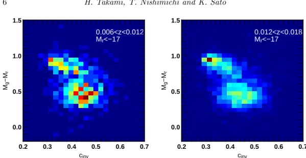
called a (inverse) concentration index listed in the NYU-VAGC as an indicator of the morphology. Since early-type (elliptical) galaxies tend to fade out slowly with distance from the center, they have relatively smaller concentration indices. On the other hand, late-type (i.e., spiral and irregular) galaxies have large concentration indices. Fig. 2 shows the frequency distributions of galaxies with M

≤ −17 and the redshift ranges of 0.006 ≤ z < 0.012 (left) and 0.012 ≤ z < 0.018 (right) on parameter space of c

and M

− M

. The number of galaxies increases when the color in each cell is close to red. In both panels, the distribution of galaxies can be separated above and below M

− M

∼ 0.6. Thus, we define galaxies with M

− M

above and below 0.6 as red and blue galaxies, respectively. On the other hand, these

distributions cannot be clearly separated in the direction parallel to c

. Ref. 52)

compared the concentration indice SDSS galaxies with apparent magnitude below

0.006<z<0.012 M

<−17

0.2 0.3 0.4 0.5 0.6 0.7

0.0 0.5 1.0 1.5

cinv

Mg−Mr

0.012<z<0.018 M

<−17

0.2 0.3 0.4 0.5 0.6 0.7

0.0 0.5 1.0 1.5

cinv

Mg−Mr

Fig. 2. Number distribution of SDSS galaxies with the redshifts of 0.006 ≤ z < 0.012 (left) and 0.012 ≤ z < 0.018 (right) on c

-M

− M

plane. c

and M

− M

are the concentration parameter of galaxies (see text) and a color indicator used in this study, respectively. The number of galaxies increases from blue to red.

16.0 detected during a commissioning phase to their morphologies and found that the best criterion between early-type and late-type morphologies is c

∼ 0.35. We simply adopt this criterion for classification between early-type galaxies and late-type galaxies.

All the volume-limited subsets of galaxies are summarized in Table I.

2.3. Statistical analysis

A lot of tests of anisotropy in the arrival distribution of HECRs focus on the excess of the number of events within a circle centered by source candidates over random events. We adopt the same approach, although the statistical quantities used in this study is different. We analyzed the PAO and AGASA data by using a differential cross-correlation function which took the anisotropic apertures of these experiments and galaxy surveys into account.

The effect of their boundary should be also taken with care in this study, since areas observed by the SDSS and the AGASA are limited and non-uniform. Here, we adopt a cumulative cross-correlation function defined similarly to the differential cross-correlation function as

C

(θ) = EG(< θ) − EG

(< θ) − E

G(< θ) + E

G

(< θ)

E

G

(< θ) . (2.1)

Here, E, G, E

and G

represent HECR events, galaxies in a sample, HECR events

randomly put with number density proportional to the detector aperture, and galax-

ies randomly put following the angular selection function (e.g., survey window, bright

star mask, and so on) in the observed sky, respectively. EG(< θ) is the normalized

number of pairs between E and G within the angular distance of θ. For normaliza-

tion, the number of the pairs are divided by the product of the number of HECR

events and the number of galaxies. EG

(< θ), E

G(< θ), and E

G

(< θ) are defined

0h 24h

90

60

30

-30

-60

-90

-1 -0.5 0 0.5 1 1.5 2

0 5 10 15 20 25 30 35 40 45

Cumulative cross-correlation: Ces(θ)

θ: Separation Angle [deg]

0.001 < z < 0.006 M_r < -17 (237 galaxies)

AGASA Random

0h 24h

90

60

30

-30

-60

-90

-1 -0.5 0 0.5 1 1.5 2

0 5 10 15 20 25 30 35 40 45

Cumulative cross-correlation: Ces(θ)

θ: Separation Angle [deg]

0.006 < z < 0.012 M_r < -17 (730 galaxies)

AGASA Random

0h 24h

90

60

30

-30

-60

-90

-1 -0.5 0 0.5 1 1.5 2

0 5 10 15 20 25 30 35 40 45

Cumulative cross-correlation: Ces(θ)

θ: Separation Angle [deg]

0.012 < z < 0.018 M_r < -17 (2221 galaxies)

AGASA Random

0h 24h

90

60

30

-30

-60

-90

-1 -0.5 0 0.5 1 1.5 2

0 5 10 15 20 25 30 35 40 45

Cumulative cross-correlation: Ces(θ)

θ: Separation Angle [deg]

0.018 < z < 0.024 M_r < -17 (7331 galaxies)

AGASA Random

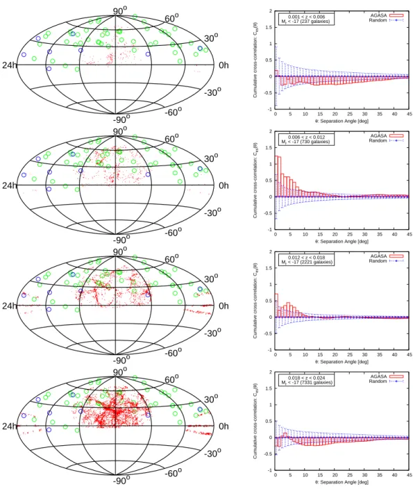
Fig. 3. left: Skymaps of the AGASA events (E > 4 × 10

eV; green circles, E > 10

eV; blue

circles) and SDSS galaxies with M

≤ −17 (red points). The redshift ranges of SDSS galaxies

are 0.001 ≤ z < 0.006, 0.006 ≤ z < 0.012, 0.012 ≤ z < 0.018, and 0.018 ≤ z < 0.024 from

top to bottom. right: Cumulative cross-correlation functions between the AGASA events and

SDSS galaxies shown in the corresponding left panels (histogram). We also show the averages

(points) and standard deviations (bars) of the cumulative cross-correlation functions calculated

from 100000 realizations of randomly distributed events in blue.

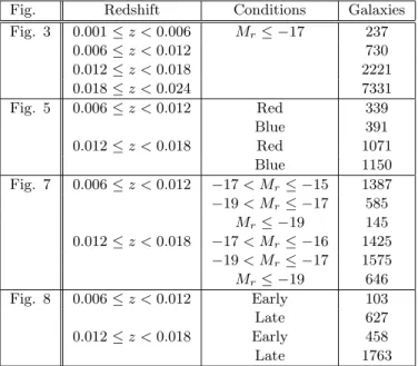
Fig. Redshift Conditions Galaxies Fig. 3 0.001 ≤ z < 0.006 M

≤ −17 237

0.006 ≤ z < 0.012 730

0.012 ≤ z < 0.018 2221

0.018 ≤ z < 0.024 7331

Fig. 5 0.006 ≤ z < 0.012 Red 339

Blue 391

0.012 ≤ z < 0.018 Red 1071

Blue 1150

Fig. 7 0.006 ≤ z < 0.012 −17 < M

≤ −15 1387

−19 < M

≤ −17 585

M

≤ −19 145 0.012 ≤ z < 0.018 −17 < M

≤ −16 1425

−19 < M

≤ −17 1575 M

≤ −19 646 Fig. 8 0.006 ≤ z < 0.012 Early 103

Late 627

0.012 ≤ z < 0.018 Early 458

Late 1763

Table I. Summary of SDSS galaxy subsamples used for analyses in this study. Parameter sets without the description of the range of M

adopt M

≤ −17. The colors of galaxies are defined as M

− M

> 0.6 (red) and M

− M

≤ 0.6 (blue). The morphology of galaxies is determined by c

≤ 0.35 (early) and c

> 0.35 (late). See text for details.

similarly to EG(< θ). E

and G

enable us to correct the non-uniformities of the HECR aperture and the galaxy sampling. This function allows us to investigate the excess of HECR events around galaxies over random events. We can also define the (angular) cumulative auto-correlation functions of galaxies similarly to Eq. 2.1 as

C

(θ) = GG(< θ) − 2GG

(< θ) + G

G

(< θ)

G

G

(< θ) . (2.2)

These functions were originally introduced by Ref. 53) for a differential auto-correlation function and by Ref. 54) for a differential cross-correlation function.

The aperture of a ground array depends on the declination of observed directions reflecting the daily rotation of the Earth. The declination dependence of the exposure (= aperture × observation time) can be analytically estimated as,

ω(δ) ∝ cos(a

) cos(δ) sin(α

) + α

sin(a

) sin(δ), (2.3) where α

is given by

α

=







0 if ξ > 1

π if ξ < −1

cos

(ξ) otherwise

, (2.4)

and

ξ ≡ cos(Θ) − sin(a

) sin(δ)

cos(a

) cos(δ) , (2.5)

if observation time is sufficiently larger than a day. Here, a

is the terrestrial latitude of a ground array and Θ is the zenith angle for a data cut because of experimental reasons. For the AGASA, a

= 35

47

and Θ = 45

.

The E

sample in Eq. 2.1 is generated following Eq. 2.3. We set the number of E

events to be 200,000 in order that the distribution of random events reflects the AGASA aperture sufficiently.

The survey area of the SDSS is also limited and complicated due to masks.

The SDSS observes about one fifth of the whole sky and the depth of observations slightly depends on directions. We take account of these effects by distributing random galaxies (i.e., G

in Eq. 2.1) following the angular selection function. We use mangle software

to do so. We distribute at least twenty times more random galaxies than the real ones, which is an usual choice. We confirmed that these particular choices of the number of random events and random galaxies do not affect the results.

The significance of positive correlation is estimated by comparing a cumulative cross-correlation function calculated from the AGASA events to that calculated from randomly distributed events with the same number of events as that of the AGASA events. We generate 100000 realizations of random events and calculate a cumula- tive cross-correlation function for every realization. Then, we count the number of realizations in which the value of the cumulative cross-correlation function is larger than that calculated from the AGASA data at every θ, and the number is divided by 100000. This number gives the probability that the correlation realized by the AGASA data within θ is realized from randomly distributed events by chance. How- ever, this probability is not a real chance probability when we scan the probability over θ. Since the scan is regarded as trials, the chance probability includes a trial factor. Thus, in order to estimate the true detection probability of the positive cor- relation, we must compensate this probability by a trial factor. In other words, the probability must be penalized.

In Section 3.1, 3.2, and 3.3, we search for the potential signals of the positive correlation and discuss their dependence on the properties of galaxies with non-penalized probability. Then, we estimate penalty factors in all the cases tested in the three sections, and evaluate the true detection probabilities of the positive correlation in Section 3.4. Then, we will check the de- pendence discussed in the former three sections based on the penalized probabilities.

Note that since the other parameters are set a priori, we need not consider statistical penalty from them.

§ 3. Results 3.1. Dependence on redshift

The left panels of Fig. 3 show the positions of galaxies (dots) and the arrival directions of the AGASA events (circles) for the four redshift ranges of galaxies:

0.001 ≤ z < 0.006, 0.006 ≤ z < 0.012, 0.012 ≤ z < 0.018, and 0.018 ≤ z < 0.024

from top to bottom, for visibility. Events with energies beyond 10

eV, are shown

as blue circles. The distributions of galaxies are highly structured; we can find the

filamentary structures and clusters of galaxies. We see that more than ten events

correlate with the filamentary structures by eye, despite that only about a half of events remains inside the region where the SDSS covers. On the other hand, the AGASA events do not correlate with Virgo cluster and Coma cluster, which are seen at around the center of the top panel and the bottom panel, respectively. The lack of the correlation with Virgo cluster was already pointed out both for the PAO events

and for the AGASA events.

Whether the AGASA events globally correlate with galaxy distribution or not can be quantified by cumulative cross-correlation functions shown in the right panels, which correspond to the left panels. For comparison, we also show the cumulative cross-correlation functions between events randomly distributed with being compat- ible to the geometry of the AGASA exposure and the same galaxies with error bars.

We simulated the same number of random events as the AGASA data 100000 times and calculated a cross-correlation function for each event set. Then, we estimated the averages (crosses) and standard deviations of the cross-correlation functions (er- ror bars). These standard deviations can be regarded as 1 σ statistical errors if the fluctuation of a cumulative cross-correlation function follows the Gaussian dis- tribution. The cumulative cross-correlation functions calculated from the data are in excess of the cumulative cross-correlation functions predicted by the randomly distributed event sets at small angular scale in the cases of 0.006 ≤ z < 0.012 and 0.012 ≤ z < 0.018. On the other hand, positive excess is not found for 0.001 ≤ z < 0.006 and 0.018 ≤ z < 0.024 at small angular scale.

10^-2 10^-1 10⁰

0 20 40 60 80 100 120 140 160 180

Chance Probability

θ: Separation Angle [deg]

68% C.L.

90% C.L.

95% C.L.

0.001 < z < 0.006 0.006 < z < 0.012 0.012 < z < 0.018 0.018 < z < 0.024

Fig. 4. Probabilities that the positive corre- lations of the AGASA events and SDSS galaxy sets within the 4 redshift ranges is reproduced from randomly distributed events by chance as a function of θ. Dotted lines represent 68% C.L., 90% C.L., and 95% C.L..

The significance of these positive correlations in an angular bin can be es- timated by using the method described in Section 2.3. Fig. 4 shows the chance probabilities that the correlation sig- nals of the AGASA data are produced from randomly distributed events for θ = 2

, 3

, · · · , 179

. Note that θ = 1

and 180

are not considered because the chance probabilities in these bins are physically meaningless. The accu- racy to determine the arrival directions of HECRs above 4 × 10

eV by the AGASA is larger than 1

(1.8

). A cumulative cross-correlation function is 0 at θ = 180

by definition. The chance probabilities are less than 5% at small angular scale (≤ 7

) in 0.006 ≤ z <

0.012 and 0.012 ≤ z < 0.018. These are the potential signals of positive correla-

tion which reflect the fact that ∼ 10 events seem to correlate with the filamentary

structure of galaxies in the left panels of Fig. 3. In the following two sections, we

focus on galaxies in these two redshift ranges and test the dependence of the cross-

correlation on the properties of galaxies, i.e., color, r-band absolute magnitude, and

morphology.

3.2. Dependence on the color of galaxies

-1 -0.5 0 0.5 1 1.5 2 2.5 3

0 5 10 15 20 25 30 35 40 45

Cumulative cross-correlation: Ces(θ)

θ: Separation Angle [deg]

0.006 < z < 0.012, M_r < -17 M_g - M_r > 0.6 (Red) (339 galaxies)

AGASA Random

-1 -0.5 0 0.5 1 1.5 2 2.5 3

0 5 10 15 20 25 30 35 40 45

Cumulative cross-correlation: Ces(θ)

θ: Separation Angle [deg]

0.006 < z < 0.012, M_r < -17 M_g - M_r < 0.6 (Blue) (391 galaxies)

AGASA Random

Fig. 5. Cumulative cross-correlation functions between the AGASA events and red (left) and blue (right) galaxies with 0.006 ≤ z < 0.012 (histogram). The points and error bars are the average and standard deviation of cumulative cross-correlation functions calculated from random events.

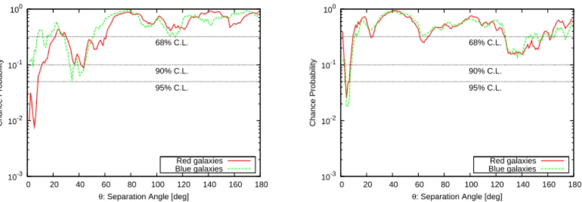
10^-3 10^-2 10^-1 10⁰

0 20 40 60 80 100 120 140 160 180

Chance Probability

θ: Separation Angle [deg]

68% C.L.

90% C.L.

95% C.L.

Red galaxies Blue galaxies

10^-3 10^-2 10^-1 10⁰

0 20 40 60 80 100 120 140 160 180

Chance Probability

θ: Separation Angle [deg]

68% C.L.

90% C.L.

95% C.L.

Red galaxies Blue galaxies

Fig. 6. Same as Fig. 4, but for red (M

−M

> 0.6; red) and blue (M

− M

≤ 0.6; green) galaxies with 0.006 ≤ z < 0.012 (left) and 0.012 ≤ z < 0.018 (right).

Fig. 5 shows the cumulative cross-correlation functions of the AGASA events with red (left) and blue (right) galaxies within 0.006 ≤ z < 0.012. The cumulative cross-correlation functions calculated from random events are also plotted. The cross-correlation function of the data is in excess of that of random events in the case of red galaxies, while the data is consistent with random events for blue galaxies within error bars. This fact can be also observed in the plot of chance probabilities (the left panel of Fig. 6). The probability that the observed positive correlation is realized from randomly distributed events by chance is less than 5% at small angular scale for the red galaxies. The same analysis is applied to galaxies within 0.012 ≤ z < 0.018 (the right panel of Fig. 6), but the difference between red and blue galaxies is small, although both the chance probabilities are less than 5% at

∼ 5

.

3.3. Dependence on other galaxy parameters

Following the former section, we test the dependence on the other two galaxy parameters, r-band absolute magnitude and morphology.

Fig. 7 is the same as Fig. 6, but for the dependence on r-band absolute mag- nitude of galaxies within 0.006 ≤ z < 0.012 (left) and 0.012 ≤ z < 0.018 (right), respectively. In the left panel, all the three galaxy samples show the chance proba- bility less than 5% at small angular scale, but the difference among them is small.

On the other hand, the chance probabilities seem to be smaller for brighter galaxies in the right panel.

10^-2 10^-1 10⁰

0 20 40 60 80 100 120 140 160 180

Chance Probability

θ: Separation Angle [deg]

68% C.L.

90% C.L.

95% C.L.

-17 < M_r < -15 -19 < M_r < -17 M_r < -19

10^-2 10^-1 10⁰

0 20 40 60 80 100 120 140 160 180

Chance Probability

θ: Separation Angle [deg]

68% C.L.

90% C.L.

95% C.L.

-17 < M_r < -16 -19 < M_r < -17 M_r < -19

Fig. 7. left: Same as Fig. 4, but for galaxies with −17 < M

≤ −15 (red), −19 < M

≤ −17 (green), and M

≤ −19 (blue) in the redshift range of 0.006 ≤ z < 0.012. right: Same as Fig. 4, but for galaxies with −17 < M

≤ −16 (red), −19 < M

≤ −17 (green), and M

≤ −19 (blue) in the redshift range of 0.012 ≤ z < 0.018.

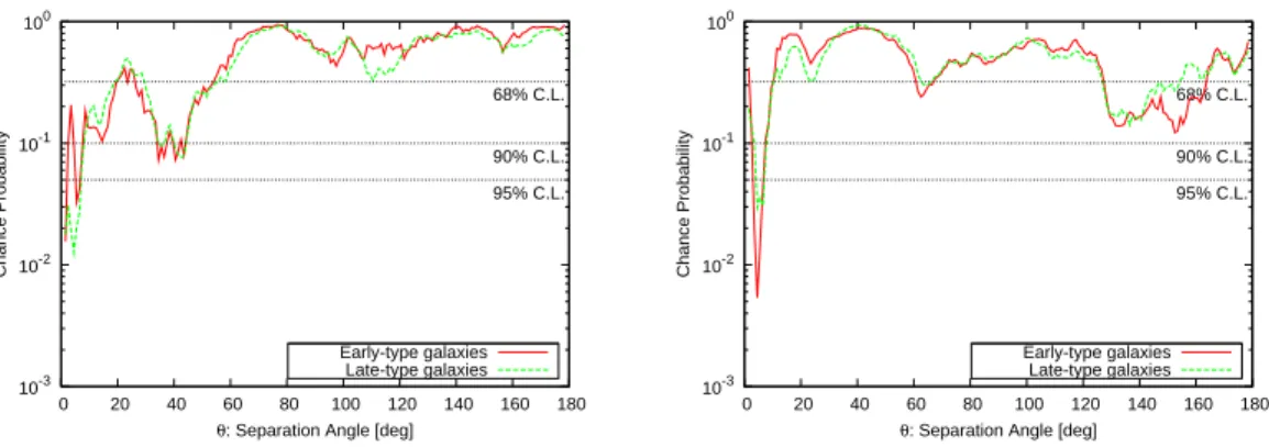
Next, we consider the morphology dependence of the cross-correlation. Fig. 8 is the same as Fig. 7, but the original galaxy samples are divided into early-type galaxies and late-type galaxies. In the range of 0.006 ≤ z < 0.012 (left), the chance probability for late-type galaxies is smaller than that for early-type galaxies at small angular scale, but not so clear. On the other hand, a positive correlation signal of early-type galaxies is stronger than that of late-type galaxies in the range of 0.012 ≤ z < 0.018 (right).

3.4. Penalized Probability

We investigated the potential signals of the positive correlation in the former

three sections by scanning the chance probability that the correlation signals of

the AGASA events are realized from randomly distributed events by chance over

angular distance. These angular scanning means that we made 178 statistical trials

by different angular scale. Thus, it is possible that more than 95% C.L. correlation

signals discussed in the former three sections result from the fluctuation of randomly

distributed events. In this case, the significance of the correlation signals is expected

to be lower in reality. In this section, we estimate the true significance of the potential

positive correlation signals found in the former three sections taking trial factors

(penalty factors) into account following the methods discussed in literature (e.g.,

Refs. 40), 58)).

10^-3 10^-2 10^-1 10⁰

0 20 40 60 80 100 120 140 160 180

Chance Probability

θ: Separation Angle [deg]

68% C.L.

90% C.L.

95% C.L.

Early-type galaxies Late-type galaxies

10^-3 10^-2 10^-1 10⁰

0 20 40 60 80 100 120 140 160 180

Chance Probability

θ: Separation Angle [deg]

68% C.L.

90% C.L.

95% C.L.

Early-type galaxies Late-type galaxies

Fig. 8. Same as Fig. 4, but for early-type (red) and late-type (blue) galaxies with 0.006 ≤ z < 0.012 (left) and 0.012 ≤ z < 0.018 (right).

0 0.02 0.04 0.06 0.08 0.1

-5 -4 -3 -2 -1 0

Frequency

Minimum Probability Isotropic AGASA data

Fig. 9. Distribution of p

calculated from randomly distributed events (red). As for galaxies to test correlation, early type galaxies located at 0.012 ≤ z < 0.018 (used in Fig. 8) are adopted. The green line is p

obtained by the AGASA events.

In this case, the probability that the ob- served correlation appears from randomly distributed events by chance is 9.5 × 10

(see also Table II).

The probability that a signal p

, which is the minimum chance probabil- ity in each analysis performed in the former three sections, is produced from isotropic distribution by chance (statis- tical fluctuations) can be estimated as follows. We generate a set of isotrop- ically distributed HECR events with the same number as the number of the AGASA events. To this event set, we perform the same analysis as in the for- mer three sections and derive the mini- mum chance probability p

. In gen- eral, the angular scale to give p

is different from that of p

. If p

<

p

, this is the case where randomly distributed events could produce the ob- served signals by fluctuation. We repeat this process 50000 times and count the number of realizations in which p

<

p

(i = 1, 2, · · · , 50000), then which is divided by 50000. This is the probability that the observed positive correlation is realized by fluctuations. In other words, one minus this probability is the true significance of the detection of positive correlation.

We confirmed that the 50000 trials were enough to estimate the penalized signifi- cance accurately. A histogram of the distribution of p

is shown in Fig. 9 to help our understanding. A galaxy sample used in this figure is the same as that used in the right panel of Fig. 8. The green line, located at the left side of the peak, is the minimum chance probability p

estimated in the right panel of Fig. 8. The area in the left side of the green line corresponds to the probability that p

is realized by chance.

The penalized probabilities of all the cases investigated in the former three sec-

tions are tabulated on Table II. We can find that the strongest correlation appears for early-type galaxies within 0.012 ≤ z < 0.018 (90% C.L.). The other penalized chance probabilities are more than 10%, but the difference of the penalized probabil- ities between the properties of galaxies indicates the dependence of the correlation on the properties. The dependence found in the table is similar to the results from the discussions using non-penalized probabilities in the former three sections. For dependence on redshifts (discussed in Fig. 3), penalized significance is clearly higher in 0.006 ≤ z < 0.012 and 0.012 ≤ z < 0.018 than in the others. For the de- pendence on the color of galaxies, red galaxies correlates with the AGASA events stronger than blue galaxies in the redshift range of 0.006 ≤ z < 0.012. Brighter galaxies produce larger significance of the correlation in 0.012 ≤ z < 0.018, whereas the dependence is not clear at 0.006 ≤ z < 0.012. The correlation with early-type galaxies is stronger in 0.012 ≤ z < 0.018, but the morphology dependence is not clear in 0.006 ≤ z < 0.012. Thus, the dependence of the correlation signals on the properties of galaxies is not common in the redshift ranges, and therefore unclear at present. However, as discussed in the next section, each population of HECR source candidates has characteristic host galaxies. The dependence searches of the positive correlation will be a powerful tool to find HECR sources as the number of detected HECR events increases.

Fig. Redshift Conditions Penalized p

Fig. 3 0.001 ≤ z < 0.006 M

≤ −17 0.94

0.006 ≤ z < 0.012 0.23

0.012 ≤ z < 0.018 0.23

0.018 ≤ z < 0.024 0.94

Fig. 5 0.006 ≤ z < 0.012 Red 0.17

Blue 0.65

0.012 ≤ z < 0.018 Red 0.31

Blue 0.19

Fig. 7 0.006 ≤ z < 0.012 −17 < M

≤ −15 0.27

−19 < M

≤ −17 0.29

M

≤ −19 0.28 0.012 ≤ z < 0.018 −17 < M

≤ −16 0.45

−19 < M

≤ −17 0.32

M

≤ −19 0.15 Fig. 8 0.006 ≤ z < 0.012 Early 0.30

Late 0.24

0.012 ≤ z < 0.018 Early 9.5 × 10

Late 0.34

Table II. Penalized probabilities. The meaning of the left three column is the same as in Table I.

Finally, we comment on another possible statistical penalty originating from

the number of trial catalogue discussed in literature.

If we test the correlation

between HECRs and the matter distribution of the Universe, the statistical penalty

also should be considered because a galaxy catalog is one realization of the matter

distribution. In other words, for instance, it is regarded as two (dependent) trials to

use two galaxy catalogue. On the other hand, this paper focuses on the correlation

between HECRs and galaxies, and examines the dependence of the correlation on the various intrinsic properties of galaxies by using galaxy subsamples constructed from a priori criteria, instead of searching for the possible strongest signal of the correlation by repeating trials over different galaxy subsamples. Thus, an additional statistical penalty is not necessary. Accordingly, our results claim not the correlation with the matter distribution but the correlation with the galaxies.

§ 4. Discussion

In Section 3.1, we found that the cumulative cross-correlation functions between AGASA events and the SDSS samples of galaxies in 0.006 ≤ z < 0.012 and 0.012 ≤ z < 0.018 are in excess of those calculated from random events within ∼ 10

. The strongest potential signals also appeared at ∼ 5

, although the penalized significance of these signals is not so large (77%). These imply small deflections (∼ 5

) during the propagation of HECRs.

HECRs are inevitably affected by a GMF. A GMF consists of a coherent com- ponent following the spiral arm of Milky Way with turbulent components,

though the details of its structure is controversial at present.

For protons, the coher- ent component dominantly contributes to the deflections of HECRs due to its long coherent length, and can weaken the correlation between HECRs and source dis- tribution because the spiral structure is generally independent of the distribution of galaxies in extragalactic space. A bisymmetric GMF model widely-adopted for HECR propagation in Galactic space

predicts deflections less than 10

for protons above 10

eV

and that a typical angular scale at which HECR-to-source correlation is expected to be ∼ 5

,

which is comparable with the angular scale giving the potential correlation signals. Thus, the positive cross-correlations support proton-dominated composition, which is consistent with the result of the HiRes, a HECR observatory in the northern hemisphere.

-1 0 1 2 3 4 5 6 7 8

0 5 10 15 20 25 30

Cumulative auto-correlation function: Cg(θ)

Separation angle [deg]

SDSS (0.001 < z < 0.006) SDSS (0.006 < z < 0.012) SDSS (0.012 < z < 0.018) IRAS (z<0.018)

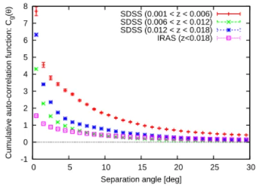
Fig. 10. Angular cumulative auto-correlation functions of galaxies in our samples used in Fig. 3. For comparison, the cumulative auto-correlation function of IRAS galaxies adopted in Ref. 23) is also shown. The er- ror bars are estimated from random distri- bution following the observed area of the SDSS and IRAS.

The signals of the cross-correlation

functions obtained in Section 3.1 is more

positive than the result of our previ-

ous analysis using IRAS galaxies, in

which the cross-correlation function of

the AGASA events is consistent with

that calculated from random events

within 1σ error.

Although depending

on several difference between the galaxy

samples, e.g., wavebands, flux limits,

observed directions, the stronger cor-

relation signal possibly originates from

galaxies at small angular scale. Fig. 10

compares the cumulative angular auto-

correlation functions of galaxies used in

Fig. 3 and the same function of a galaxy

sample used in our previous study. The

error bars are estimated from random event generation by putting random galaxies with the same number as the number of the real galaxies following the observed area of the SDSS and IRAS 100 times and then by estimating the standard deviation of 100 auto-correlation functions as 1σ errors. Note that we adopt these criteria on redshifts to directly compare this study with the previous study although the redshift ranges are different. This figure shows that the SDSS samples are con- centrated at small angular scale stronger than the IRAS sample. These positive auto-correlations at small angular scale could be positively working.

The deflection of HECRs by IGMFs depends on their propagation distance. For a random IGMF, the total deflection angles of HECRs, ϕ(ǫ, D), are proportional to the square root of their propagation distance (e.g., Ref. 65)),

ϕ(ǫ, D) ≃ 2.5

Zǫ

D

B

l

, (4.1) where ǫ

= ǫ/10

eV, D

= D/100 Mpc, B

= B/10

G and l

= l

/1 Mpc are the energy of HECRs, their propagation distance, the strength of the IGMF, the coherent length of the IGMF, respectively. The trajectories of HECRs from a more distant source are deflected stronger. The cumulative cross-correlation of the AGASA events and galaxies with 0.018 ≤ z < 0.024 consistent with that of random events could be interpreted as the effect of the IGMF as well as the lack of correlation with IRAS galaxies with z > 0.018 shown in Ref. 23). On the other hand, this interpretation does not apply to 0.001 ≤ z < 0.006, the nearest galaxy sample. This implies that there is not strong HECR sources within z = 0.006 (∼ 25 Mpc in the concordance cosmology) in the field observed by the SDSS.

IGMFs could trick us in some cases and could generate spurious correlation even for light-nuclei dominated composition.

In this scenario, HECRs can be scattered toward the Earth by strongly magnetized structures, e.g., clusters of galaxies, lobes of radio galaxies, and therefore the arrival directions of HECRs do not necessarily point out the positions of their sources although the correlation between HECRs and galaxy distribution can be detected. Ref. 66) reported that about 50% of the PAO events published in Ref. 19) could be such spurious correlations. A similar phenomena is reported by Ref. 67) based on simulations of propagation of protons taking a sophisticated and simulated IGMF model

into account. The latter also show that predicted angles between the arrival directions of protons and AGN-like objects defined in their simulations are consistent with the correlation angles derived by the PAO

even if there are true sources far from the AGN-like objects. If the spurious correlation is dominantly realized in the Universe, it is difficult to identify HECR sources by the arrival directions of HECRs. Note that such a phenomenon strongly depends on IGMF modelling including large uncertainty at present. IGMF models by Refs. 69) and 70) predict smaller deflections of HECRs and show spurious correlation much less than the former two IGMF models. The latter IGMF model even predicts the correlation between HECRs and their sources in local Universe within a few degree for proton-dominated composition.

The nature of galaxies which correlates with HECR events is a hint of HECR

sources if the spurious correlation is not realized. Based on this motivation, we inves-

tigated the dependence of the correlation between the AGASA events and galaxies on galaxy parameters, such as color, r-band absolute magnitude, and morphology.

We adopted M

− M

to divide galaxies into red galaxies and blue galaxies. This value is a good indicator of contents of galaxies because the 4000 ˚ A break of galaxies is included in g-band. This spectral break is a characteristic feature of long-lived stars like K-type stars. Thus, strong star forming and a number of young (massive) stars are not expected in galaxies with a strong spectral break at ∼ 4000 ˚ A, i.e.

relatively red galaxies for this color definition. The dependence of the correlation of HECRs and galaxies on their colors informs us of the epochs of HECR generation in the history of galaxies and environment which includes HECR sources. We sum- marize the current understanding of the host galaxies of HECR source candidates, such as GRBs, magnetars, and AGN.

GRBs (at least long-duration ones) are thought to be related to explosions of massive stars at the end of their life.

Many observations have indicated that the typical nature of GRB host galaxies is faint star-forming galaxies dominated by a young stellar population

and tends low luminosities,

low masses,

and therefore low metallicities.

Reflecting these facts, the colors of GRB host galaxies tend to be blue,

even in nearby Universe.

Note that the definition of the color of galaxies in Ref. 77), R − K, is essentially the same as the M

− M

color, because both are indicators of old (long-lived) star population in galaxies. Morpho- logically, GRBs correlate with irregular or late-type galaxies,

but a recent study which use the largest sample of GRB host galaxies reports no compelling evidence that GRB host galaxies are peculiar galaxies in the point of their morphologies.

We should take care of the time-delay of HECRs during their propagation in intergalactic space when we discuss whether GRBs are HECR sources or not from the nature of galaxies which correlate with HECR events. The color of GRB host galaxies is expected to become red after massive stars are exploded. In other words, the host galaxies are no longer blue at present if the time-delay is larger than the lifetime of massive stars. The masses of GRB progenitors are thought to be larger than ∼ 25M

or typically ∼ 40M

to require black hole formation by stellar core collapse under a collapser model.

The typical main sequence lifetime of such massive stars is ∼ 10

yr. On the other hand, the time-delay of HECRs depends on the modelling of IGMF. In a uniformly turbulent IGMF, which is a simple case, the time-delay, τ

(ǫ, D) is estimated as

τ

(ǫ, D) ∼ 10

Zǫ

D

B

l

yr, (4.2)

and this allows us to observe blue host galaxies. However, IGMF is structured in the

Universe. Regions in which have stronger magnetic fields can produce larger time-

delay. Several IGMF models predict the time-delay of HECRs sufficiently smaller

than the lifetime of massive stars.

If IGMF indicated by these works is realized

in the Universe, the discussion on colors of the correlated galaxies does not lose its

efficiency. Other IGMF models predict that a significant fraction of HECRs has time-

delay larger than ∼ 10

yr even for protons.

In this case, since the trajectories

of such HECRs are highly deflected, the host galaxies of GRBs becomes already red

and also correlation between HECRs and their sources itself can disappear. Thus, it

is difficult to confirm the GRB origin of HECRs from correlation studies of HECRs if these strong IGMF models are realized.

The production mechanism of magnetars is still controversial, but magnetars are mainly thought to be produced through core-collapse of massive stars because a large fraction of magnetar candidates correlate with supernova remnants or mas- sive stellar cluster

(see Ref. 86) for a review). All the magnetar candidates are detected inside or very close to our galaxy, and therefore the nature of the host galaxies of magnetars is also poorly known. Based on the hypothesis that magnetars are generated by core-collapse of massive stars, they are often produced in star- forming galaxies. GRB060218 (sometimes categorized into X-ray flush) is a possible candidate of a GRB leaving a magnetar, classified into low-luminosity GRBs, and the progenitor mass is estimated as ∼ 20M

,

which is smaller than that of GRBs which leave black holes (high-luminosity GRBs). It was theoretically predicted that low-luminosity GRBs accompany the production of magnetars.

Thus, the host galaxies of newly born magnetars could be redder than that of high-luminosity GRBs.

Note that low-luminosity GRBs themselves are also possible to accelerate particles up to the highest energies.

AGN which are theoretically motivated as HECR source candidates are classified into radio galaxies, which are dominated by non-thermal radiation. The host galaxies of such AGN have been well investigated and have early-type morphology and red color.

The strongest signal of the positive correlation obtained in this study originated from early-type galaxies at 0.012 ≤ z < 0.018. This signal indicates that some kinds of AGN activity are related to HECR generation among known source candidates.

However, we could not find clear common dependence between the two redshift ranges, e.g., the AGASA events correlated with red galaxies stronger tha blue galax- ies in 0.006 ≤ z < 0.012 while this was not clear at 0.012 ≤ z < 0.018. Thus, we cannot make a clear conclusion of HECR sources at present. The discussion above was based on the results from very limited detected events. Increasing the number of detected events can allow us to obtain a clear conclusion.

Finally, we discuss a fraction for HECRs emitted from sources at a distance to

contribute to the total flux. Fig. 11 shows the cumulative fraction of the HE proton

flux arriving from sources with distances represented as the horizontal axis to the

total flux observed at the Earth. We assume that HECR sources are distributed

uniformly and a ΛCDM cosmology with H

= 71 km s

Mpc

, Ω

= 0.3, and

Ω

= 0.7, as the Hubble parameter, the ratio of matter density to the critical den-

sity, and the ratio of cosmological constant to the critical density, respectively. These

cumulative fractions are calculated under the continuous energy-loss approximation

of Bethe-Heitler pair creation

and photopion production.

The cumulative frac-

tions are calculated under several assumptions on the nature of HECR sources; a

spectral index α of HECR emission spectrum and a cosmological evolution factor

of HECR source density with a shape of (1 + z)

, and rectilinear propagation (ne-

glecting IGMFs). We can see that the fraction of protons arriving at the Earth

from sources within 100 Mpc is only 10-20 % for protons with energies of 10

eV

(left). Even for protons with 10

eV (right), the fraction is maximally ∼ 40 %.

0 0.1 0.2 0.3 0.4 0.5 0.6 0.7 0.8 0.9 1

0 100 200 300 400 500

Cumulative fraction

Comoving distance [Mpc]

E_p=10^19.6 eV

α=2.6, m=0.0 α=2.5, m=3.0 α=2.0, m=0.0 α=2.0, m=3.0

0 0.1 0.2 0.3 0.4 0.5 0.6 0.7 0.8 0.9 1

0 50 100 150 200 250 300

Cumulative fraction

Comoving distance [Mpc]

E_p=10^19.8 eV

α=2.6, m=0.0 α=2.5, m=3.0 α=2.0, m=0.0 α=2.0, m=3.0

Fig. 11. Cumulative fractions of the flux of protons arriving from sources with distances represented as the horizontal axis to the total flux of protons observed at the Earth with energies of 10

eV (left) and 10

eV (right), respectively. HECR sources are assumed to be distributed uniformly.

α is a spectral index of HECR emission and m is a index of a power-law cosmological evolution scenario proportional to (1 + z)

.

However, IGMFs could more deflect the trajectories of HECRs emitted from more distant sources and therefore the cross-correlation signal between arriving HECRs and distant sources may be weaken as discussed above. Therefore, it is natural to focus on the cross-correlation of HECRs and nearby galaxy distribution. In addition, sources in redshift for every 0.006, which corresponds to every ∼ 25 Mpc, can equally contribute to the total HECR flux up to z = 0.024 because the cumulative functions can be approximated by straight lines below ∼ 100 Mpc.

§ 5. Conclusion

In this study, we investigated the correlation between the arrival directions of

HECRs detected in the northern sky (the AGASA data) and volume-limited samples

of galaxies observed by the SDSS. We found that the excess of the cumulative cross-

correlation functions between the AGASA events and SDSS galaxies over random

HECR events at small angular scale in the redshift ranges of 0.006 ≤ z < 0.012 and

0.012 ≤ z < 0.018. These cross-correlation signals imply light composition at the

highest energy. Then, we examined the dependence of the correlation on the prop-

erties of galaxies in these two redshift ranges. The properties of galaxies correlating

with HECRs can give us a hint of HECR sources unless the spurious correlation

is dominated, as galaxies hosting HECR sources are expected to be characteristic

features (discussed in Section 4). The strongest correlation signal originated from

early-type galaxies in 0.012 ≤ z < 0.018 at 90% C.L. (penalized significance) and the

AGASA events have excess over random events at small angular scale for red galax-

ies rather than blue galaxies at 0.006 ≤ z < 0.012, but we could not find common

dependence between the two redshift ranges probably due to the limitation of the

number of HECR events. In order to obtain a clear conclusion, the more number of

HECR events should be adopted for the analysis. Data accumulation in the northern

sky is in progress. The total exposure of the Telescope Array have already reached