Chapter 3 TROPICAL CYCLONE MOTION

Chapter 3

TROPICAL CYCLONE MOTION

The prediction of tropical cyclone motion has improved dramatically during the last decade as has our understanding of the mechanisms involved. Some of the basic aspects of tropical cyclone motion can be illustrated in terms of barotropic theory, which assumes that the vortex structure is independent of height. We begin first by examining this theory and go on in a following section to examine baroclinic aspects of motion.

3.1 Vorticity-streamfunction method

The vorticity-streamfunction method is a powerful way of solving two-dimensional flow problems for a homogeneous, incompressible fluid. It is conventional to choose a rectangular coordinate system (x, y), with x pointing eastwards and y pointing northwards. For two-dimensional motion in the x-y-plane, the relative vorticity, ζ, is defined as ∂v/∂x − ∂u/∂y and satisfies the equation

∂

∂t (ζ + f) + u ∂

∂x (ζ + f) + v ∂

∂y (ζ + f) = 0, (3.1)

where u and v are the velocity components in the x and y directions, respectively.

For an incompressible fluid, the continuity equation is

∂u

∂x + ∂v

∂x = 0, (3.2)

and accordingly there exists a streamfunction ψ such that u = − ∂ψ

∂y , v = ∂ψ

∂x , (3.3)

and

ζ = ∂

ψ

∂x

+ ∂

ψ

∂y

, (3.4)

70

Equation (3.1) is a prediction equation for the absolute vorticity ζ + f and states that this quantity is conserved following columns

of fluid. Equation (3.4) can be used as an expression for calculating ζ if ψ is known, or, alternatively, as an elliptic second-order partial differential equation for ψ if ζ is known. When ψ is known, u and v can be calculated from the expressions (3.3).

In a few simple cases it may be possible to obtain an analytic solution of Eqs.

3.1, 3.3 and 3.4, but in general we must resort to numerical methods. The system of equations can be solved numerically using the following steps:

• From a given initial distribution of ψ at, say t = 0, we can calculate the initial velocity distribution from Eq. (3.3) and the initial vorticity distribution from Eq, (3.4). Alternatively, given the initial vorticity distribution, we can solve Eq. (3.4) for the initial streamfunction distribution ψ and then calculate the initial velocity distribution from Eq. (3.3).

• We are now in a position to predict the vorticity distribution at a later time, say t = ∆t, using Eq. (3.1).

• Then we can solve Eq. (3.4) for the streamfunction distribution ψ at time ∆t and the new velocity distribution from Eq. (3.3).

• We now repeat this procedure to extend the solution forward to the time t = 2∆t, and so on.

3.2 The partitioning problem

An important issue that arises in the study of tropical cyclone motion is the so-called partitioning problem, i.e. the problem of deciding what is the cyclone and what is its environment. Of course, Nature makes no distinction so that any partitioning that we make to enable us to discuss the interaction between the tropical cyclone and its environment is necessarily non-unique.

Various methods have been proposed to isolate the cyclone from its environment and each may have their merits in different applications. One obvious possibility is to define the cyclone as the azimuthally-averaged flow about the vortex centre, and the residual flow (i.e. the asymmetric component) was defined as ”the environment”.

But then the question arises: which centre? As we show below, the location of the minimum surface pressure and the centre of the vortex circulation at any level are, in general, not coincident. The pros and cons of various methods are discussed by Kasahara and Platzman (1963) and Smith et al. (1990). Many theoretical studies consider the motion of an initially symmetric vortex in some analytically-prescribed environmental flow. If the flow is assumed to be barotropic, there is no mechanism

1

In a two-dimensional flow, there is no dependence of u, v, or ζ on the z-coordinate and we can

think of the motion of thin columns of fluid of uniform finite depth, or infinite depth, analogous to

fluid parcels in a three-dimensional flow.

for vortex intensification. In this case it is advantageous to define the vortex to be the initial relative vorticity distribution, appropriately relocated, in which case all the flow change accompanying the vortex motion resides in the residual flow that is considered to be the vortex environment. We choose also the position of the relative vorticity maximum as the ’appropriate location’ for the vortex. An advantage of this method (essentially Kasahara and Platzman’s method III) is that all the subsequent flow changes are contained in one component of the partition and the vortex remains

”well-behaved” at large radial distances. Further, one does not have to be concerned with vorticity transfer between the symmetric vortex and the environment as this is zero, by definition. The method has advantages also for understanding the motion of initially asymmetric vortices as discussed by Smith et al. (1990) and in Section 4.1.

The partitioning method can be illustrated mathematically as follows. Let the total wind be expressed as u = u

+ U, where u

denotes the symmetric velocity field and U is the vortex environment vorticity, and define ζ

= k · ∇ ∧ u

and Γ = k · ∇ ∧ U, where k is the unit vector in the vertical. Then Eq. (3.1) can be partitioned into two equations:

∂ζ

∂t + c(t) · ∇ζ

= 0, (3.5)

and ∂ Γ

∂t = −u

· ∇(Γ + f ) − (U − c) · ∇ζ

− U · ∇(Γ + f ), (3.6) noting that u

· ∇ζ

= 0, because for a symmetric vortex u

is normal to ∇ζ

. Equation (3.5) states that the symmetric vortex translates with speed c and Eq. (3.6) is an equation for the evolution of the asymmetric vorticity. Having solved the latter equation for Γ(x, t), we can obtain the corresponding asymmetric streamfunction by solving Eq. (3.4) in the form ∇

ψ

= Γ. The vortex translation velocity c may be obtained by calculating the speed U

= k ∧ ∇ψ

at the vortex centre. In some situations it is advantageous to transform the equations of motion into a frame of reference moving with the vortex

. Then Eq. (3.5) becomes ∂ζ

/∂t ≡ 0 and the vorticity equation (3.6) becomes

∂Γ

∂t = −u

· ∇(Γ + f ) − (U − c) · ∇ζ

− (U − c · ∇(Γ + f ). (3.7)

3.3 Prototype problems

3.3.1 Symmetric vortex in a uniform flow

Consider a barotropic vortex with an axisymmetric vorticity distribution embedded in a uniform zonal air stream on an f-plane. The streamfunction for the flow has the

2

See Appendix 9.1 for details.

form:

ψ(x, y) = −Uy + ψ

(r), (3.8)

where r

= (x − Ut)

+ y

. The corresponding velocity field is u = (U, 0) +

µ

− ∂ψ

∂y , ∂ψ

∂x

¶

, (3.9)

The relative vorticity distribution, ζ = ∇

ψ, is symmetric about the point (x − Ut, 0), which translates with speed U in the x-direction. However, neither the streamfunction distribution ψ(x, y, t), nor the pressure distribution p(x, y, t), are symmetric and, in general, the locations of the minimum central pressure, maximum relative vorticity, and minimum streamfunction (where u = 0) do not coincide. In particular, there are three important deductions from (3.9):

• The total velocity field of the translating vortex is not symmetric, and

• The maximum wind speed is simply the arithmetic sum of U and the maximum tangential wind speed of the symmetric vortex, V

= (∂ψ

/∂r)

.

• The maximum wind speed occurs on the right-hand-side of the vortex in the direction of motion in the northern hemisphere and on the left-hand-side in the southern hemisphere.

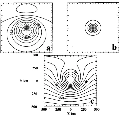
Figure 3.1 shows an example of the vorticity, streamfunction and wind speed distribution for the tropical-cyclone-scale vortex in Fig. 3.6, translating in a uniform westerly current of 10 m s

. The maximum tangential velocity is 40 m s

at a radius of 100 km.

Because the vorticity field is Galilean invariant while the pressure field and streamfunction fields are not, it is advantageous to define the vortex centre as the location of maximum relative vorticity and to transform the equations of motion to a coordinate system (X, Y ) = (x − Ut, y), whose origin is at this centre

. In this frame of reference, the streamfunction centre is at the point (0, Y

), where

U − Φ(Y

)Y

= 0, (3.10)

and Φ = ψ

(r)/r. This point is to the left of the vorticity centre in the direction of motion in the northern hemisphere. In the moving coordinate system, the momentum equations may be written in the form

∇p = ρΦ(Φ + f)(X, Y ) + ρf (0, U). (3.11) The minimum surface pressure occurs where ∇p = 0, which from (3.11) is at the point (0, Y

) where

Y

Φ(Y

)(Φ(Y

) + f ) = f U. (3.12)

3

The transformation of the equations of motion to a moving coordinate system is derived in

Appendix 9.1.

Figure 3.1: Contour plots of (a) total wind speed, (b) relative vorticity, and (c) streamlines, for a vortex with a symmetric relative vorticity distribution and maxi- mum tangential wind speed of 40 m s

in a uniform zonal flow with speed 10 m s

on an f-plane. The maximum tangential wind speed occurs at a radius of 100 km (for the purpose of illustration). The contour intervals are: 5 m s

for wind speed, 2 × 10

s

for relative vorticity and 1 × 10

m

s

for streamfunction.

We show that, although Y

and Y

are not zero and not equal, they are for practical purposes relatively small.

Consider the case where the inner core is in solid body rotation out to the radius

r

, of maximum tangential wind speed v

, with uniform angular velocity Ω = v

/r

.

Then ψ

(r) = Ωr and Φ = Ω. It follows readily that Y

/r

= U/v

and Y

/r

=

U/(v

Ro

), where Ro

= v

/(r

f ) is the Rossby number of the vortex core which

is large compared with unity in a tropical cyclone. Taking typical values: f =

5 × 10

s

, U = 10 m s

, v

= 50 ms

, r

= 50 km, Ro

= 20 and Y

=

10 km, Y

= 0.5 km, the latter being much smaller than r

. Clearly, for weaker

vortices (smaller v

) and/or stronger basic flows (larger U ), the values of Y

/r

and

Y

/r

are comparatively larger and the difference between the various centres may

be significant.

3.3.2 Vortex motion on a beta-plane

Another prototype problem for tropical-cyclone motion considers the evolution of an initially-symmetric barotropic vortex on a Northern Hemisphere β-plane in a quiescent environment. The problem was investigated by a number of authors in the late 80s using numerical models (Chan and Williams, 1987; Fiorino and Elsberry 1989; Smith et al. 1990; Shapiro and Ooyama 1990) and an approximate analytic solution was obtained by Smith and Ulrich (1990). In this problem, the initial absolute vorticity distribution, ζ + f is not symmetric about the vortex centre: a fluid parcel at a distance y

poleward of the vortex centre will have a larger absolute vorticity than one at the same distance equatorward of the centre. Now Eq. (3.1) tells us that ζ + f is conserved following fluid parcels and initially at least these will move in circular trajectories about the centre. Clearly all parcels initially west of the vortex centre will move equatorwards while those initially on the eastward side will move polewards. Since the planetary vorticity decreases for parcels moving equatorwards, their relative vorticity must increase and conversely for parcels moving polewards. Thus we expect to find a cyclonic vorticity anomaly to the west of the vortex and an anticyclonic anomaly to the east.

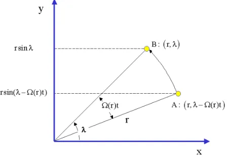
Figure 3.2: An air parcel moving in a circular orbit of radius r with angular velocity Ω(r) is located at the point B with polar coordinates (r, λ) at time t. At time t = 0 the parcel was located at point A with coordinates (r, λ − Ω(r)t). During this time it undergoes a meridional displacement r[sin λ − sin(λ − Ω(r)t)].

To a first approximation we can determine the evolution of the vorticity asymme-

tries by assuming that the flow about the vortex motion remains circular relative to

the moving vortex (we discuss the reason for the vortex movement below). Consider

an air parcel that at time t is at the point with polar coordinate (r, λ) located at

the (moving) vortex centre (Fig. 3.2). This parcel would have been at the position (r, λ − Ω(r)t) at the initial instant, where Ω(r) = V (r)/r is the angular velocity at radius r and V (r) is the tangential wind speed at that radius. The initial vorticity of the parcel is ζ

(r) + f

+ βr sin(λ − Ω(r)t) while the vorticity of a parcel at its current location is ζ(r) + f

+ βr sin λ. Therefore the vorticity perturbation ζ

(r, λ) at the point (r, λ) at time t is ζ(r) − ζ

(r), or

ζ

(r, λ) = βr[sin λ − sin(λ − Ω(r)t)]

or

ζ

(r, λ) = ζ

(r, t) cos λ + ζ

(r, t) sin λ, (3.13) where

ζ

(r, t) = −βr sin(Ω(r)t), ζ

(r, t) = −βr[1 − cos(Ω(r)t)]. (3.14) We can now calculate the asymmetric streamfunction ψ

(r, λ, t) corresponding to this asymmetry using Eq. (3.4). The solution should satisfy the boundary condition that ψ → 0 as r → ∞. It is reasonable to expect that ψ

will have the form:

ψ

(r, λ) = Ψ

(r, t) cos λ + Ψ

(r, t) sin λ, (3.15) and it is shown in Appendix 3.4.1 that

Ψ

(r, t) = − r 2

Z

r

ζ

(p, t) dp − 1 2r

Z

0

p

ζ

(p, t) dp (n = 1, 2), (3.16) The Cartesian velocity components (U

, V

) = (−∂ Ψ

/∂y, ∂Ψ

/∂x) are given by

U

= cos λ sin λ

· Ψ

r − ∂Ψ

∂r

¸

− sin

λ ∂Ψ

∂r − cos

λ Ψ

r , (3.17)

V

= cos

λ ∂ Ψ

∂r + sin

λ Ψ

r − cos λ sin λ

· Ψ

r − ∂Ψ

∂r

¸

. (3.18)

In order that these expressions give a unique velocity at the origin, they must be independent of λ as r → 0, in which case

∂ Ψ

∂r

¯ ¯

¯ ¯

r=0

= lim

r→0

Ψ

r , (n = 1, 2).

Then

(U

, V

)

=

·

− ∂Ψ

∂r

¯ ¯

¯ ¯

r=0

, ∂ Ψ

∂r

¯ ¯

¯ ¯

r=0

¸

, (3.19)

and using (3.16) it follows that

∂ Ψ

∂r

¯ ¯

¯ ¯

r=0

= − 1 2

Z

0

ζ

(p, t) dp. (3.20)

If we make the reasonable assumption that the symmetric vortex moves with the velocity of the asymmetric flow across its centre, the vortex speed is simply

c(t) =

·

− ∂Ψ

∂r

¯ ¯

¯ ¯

r=0

, ∂Ψ

∂r

¯ ¯

¯ ¯

r=0

¸

, (3.21)

which can be evaluated using (3.14) and (3.20).

The assumption is reasonable because at the vortex centre ζ À f and the gov- erning equation (3.1) expresses the fact that ζ + f is conserved following the motion.

Since the symmetric circulation does not contribute to advection across the vortex centre (recall that the vortex centre is defined as the location of the maximum rela- tive vorticity), advection must be by the asymmetric component. With the method of partitioning discussed in section 3.2, this component is simply the environmental flow by definition. The slight error committed in supposing that ζ is conserved rather than ζ + f is equivalent to neglecting the propagation of the vortex centre. The track error amounts to no more than a few kilometers per day which is negligible compared with the actual vortex displacements (e.g., see Fig. 3.6).

The vortex track, X(t) = [X(t), Y (t)] may be obtained by integrating the equa- tion dX/dt = c(t), and using (3.20) and (3.21), we obtain

· X(t) Y (t)

¸

=





1 2

R

0

nR

0

ζ

(p, t)dt o

dp

−

R

0

nR

0

ζ

(p, t)dt o

dp



 . (3.22)

With the expressions for ζ

in (3.14), this expression reduces to

· X(t) Y (t)

¸

=



 −

β R

0

r h

t −

i

dr

1 2

β R

0

r

h

i dr



 . (3.23)

This expression determines the vortex track in terms of the initial angular velocity profile of the vortex. To illustrate the solutions we choose the vortex profile used by Smith et al. (1990) so that we can compare the model results with their numerical solutions. The velocity profile V (r) and corresponding angular velocity profile Ω(r) are shown as solid lines in Fig. 3.3. The maximum wind speed of 40 m s

occurs at a radius of 100 km and the region of approximate gale force winds (> 15 m s

) extends to 300 km. The angular velocity has a maximum at the vortex center and decreases monotonically with radius. Figure 3.6 shows the asymmetric vorticity field calculated from (3.14) and the corresponding streamfunction field from (3.16) at selected times, while Fig. 3.4 compares the analytical solutions with numerical solutions at 24 h.

The integrals involved are calculated using simple quadrature. After one minute

the asymmetric vorticity and streamfunction fields show an east-west oriented di-

pole pattern. The vorticity maxima and minima occur at the radius of maximum

tangential wind and there is a southerly component of the asymmetric flow across

Figure 3.3: (left) Tangential velocity profile V (r) and (right) angular velocity profile Ω(r) for the symmetric vortex.

the vortex center (Fig. 3.4a). As time proceeds, the vortex asymmetry is rotated by the symmetric vortex circulation and its strength and scale increase. The reasons for this behaviour are discussed below. In the inner core (typically r < 200 km), the asymmetry is rapidly sheared by the relatively large radial gradient of Ω (Fig.

3.4b). In response to these vorticity changes, the streamfunction dipole strengthens and rotates also, whereupon the asymmetric flow across the vortex center increases in strength and rotates northwestwards. Even at 24 h, the asymmetric vorticity and streamfunction patterns show remarkable similarity to those diagnosed from the com- plete numerical solution of Smith et al. (1990), which can be regarded as the control calculation (see Fig. 3.5). The numerical calculation was performed on a 2000 km × 2000 km domain with a 20 km grid size. Despite the apparent similarities between the analytically and numerically calculated vorticity patterns in Fig. 3.5, the small differences in detail are manifest in a more westerly oriented stream flow across the vortex center in the analytical solution and these are reflected in differences in the vortex tracks shown in Fig. 3.6. It follows that the analytical solution gives a track that is too far westward, but the average speed of motion is comparable with, but a fraction smaller than in the control case for this entire period. Even so, it is apparent that the simple analytic solution captures much of the dynamics in the full numerical solution.

Exercises

(3.1) Starting from Eq. 3.6 and the assumptions that air parcels move in circular

orbits about the vortex centre while conserving their absolute vorticity and that

the relative advection of vortex vorticity is small, show that the asymmetric

Figure 3.4: Asymmetric vorticity (top panels) and streamfunction fields (bottom panels) at selected times: (a) 1 min, (b) 1 h, (c) 3 h, (d) 12 h. Contour intervals for ζ

are: 1 × 10

s

in (a), 5 × 10

s

in (b), 1 × 10

s

in (c), and 2 × 10

s

in (d). Contour intervals for ψ

are: 100 m

s

in (a), 6 × 10

m

s

in (b), 1 × 10

m

s

in (c), and 5 × 10

m

s

in (d). (continued overleaf)

vorticity approximately satisfies the equation:

∂ζ

∂t + Ω(r) ∂ζ

∂λ = −βrΩ(r) sin λ. (3.24) (3.2) Show that the equation

∂X

∂t + Ω(r, t) ∂X

∂λ = −βrΩ(r, t) cos λ has the solution

X = −βr(sin λ − sin(λ − ω)),

Fig. 3.4 (continued)

where

ω = Z

0

Ω(r, t

)dt

.

The analytic theory can be considerably improved by taking account of the con- tribution to the vorticity asymmetry, ζ

, by the relative advection of symmetric vortex vorticity, ζ

. This contribution is represented by the term −(U

− c) · ∇ζ

in Eq. 3.6 (the second term on the right-hand-side). Again, with the assumption that air parcels move in circular orbits about the vortex centre while conserving their absolute vorticity, ζ

satisfies the equation:

∂ζ

∂t + Ω(r) ∂ζ

∂λ = −(U

− c) · ∇ζ

, (3.25)

where the components of U

are given by Eqs. (3.17) and (3.18), and c is given by

Eq. (3.21). Further details of this calculation are given in Appendix 3.4.2. With

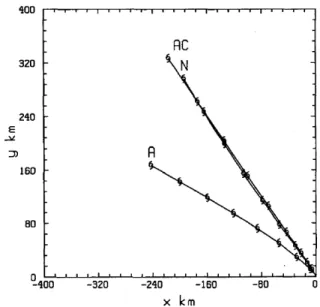
this correction there is excellent agreement between the numerically and analytically calculated tracks (compare the tracks AC and N in Fig. 3.6).

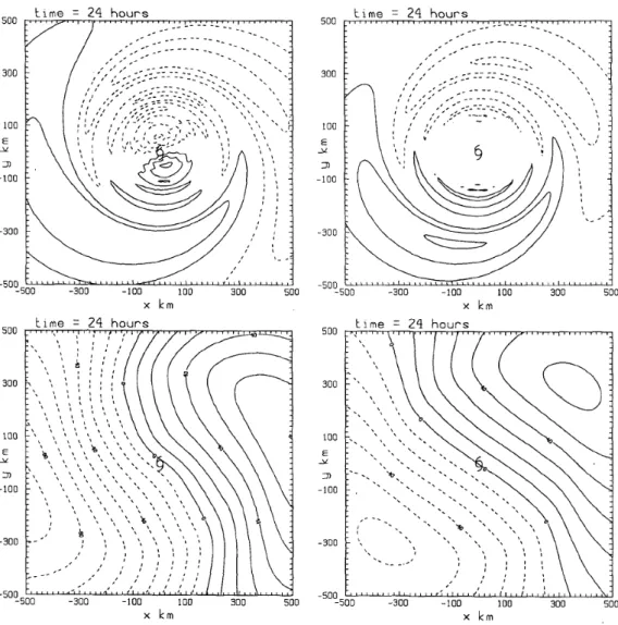
Figure 3.5: Comparison of the analytically-computed asymmetric vorticity and streamfunction fields (upper right and lower right) with those for the corresponding numerical solutions at 24 h. Only the inner part of the numerical domain, centred on the vortex centre, is shown (the calculations were carried out on a 2000 km × 2000 km domain). Contour intervals are 5 × 10

s

for ζ

and 10

m

s

for ψ

. The tropical cyclone symbol represents the vortex centre.

The foregoing analytical solution shows that the vorticity asymmetry is domi-

nated by a pair of orthogonal dipoles with different radial profiles and strengths and

that these profiles evolve with time. These profiles are characterized by the func-

tions Ψ

(r, t) in Eq. (3.15), which are shown in Fig. 3.7 at 24 h. At this time the

maximum amplitude of the vorticity asymmetry is located more than 350 km from

the vortex centre, where the tangential wind speed of the vortex is only about one

Figure 3.6: Comparison of the analytically calculated vortex track (denoted by A) compared with that for the corresponding numerical solution (denoted by N). The track by AC is the analytically corrected track referred to in the text.

quarter of its maximum value. As time proceeds, the strength of the asymmetry and the radius at which the maximum occurs continue to increase until about 60 h when the radius of the maximum stabilizes (see Smith et al. 1990, Fig. 5). This increase in the strength and scale of the gyres in the model is easy to understand if we ignore the motion of the vortex. As shown above, the change in relative vorticity of a fluid parcel circulating around the vortex is equal to its displacement in the direction of the absolute vorticity gradient times the magnitude of the gradient. For a fluid parcel at radius r the maximum possible displacement is 2r, which limits the size of the maximum asymmetry at this radius. However, the time for this displace- ment to be achieved is π/Ω(r), where Ω(r) is the angular velocity of a fluid parcel at radius r. Since Ω is largest at small radii, fluid parcels there attain their maximum displacement relatively quickly, and as expected the maximum displacement of any parcel at early times occurs near the radius of maximum tangential wind (Fig. 3.8a).

However, given sufficient time, fluid parcels at larger radii, although rotating more slowly, have the potential to achieve much larger displacements than those at small radii; as time continues, this is exactly what happens (Fig 3.8b). Ultimately, of course, if Ω(r) decreases monotonically to zero, there is a finite radius beyond which the tangential wind speed is less than the translation speed of the vortex. As the maximum in the asymmetry approaches this radius the vortex motion can no longer be ignored (see Smith and Ulrich 1990, Fig. 12).

Since the absolute vorticity is the conserved quantity in the barotropic flow prob-

lem it is instructive to examine the evolution of the isolines of this quantity as the

flow evolves. At the initial time the contours are very close to circular near the vortex

Figure 3.7: Radial profiles of Ψ

/Ψ

(n = 1, 2) at 24 hh where Ψ

is the maximum absolute value of Ψ

. Solid line is Ψ

, dashed line is Ψ

. Here, Ψ

= 4.8 × 10

m

s

; Ψ

= 4.2 × 10

m

.

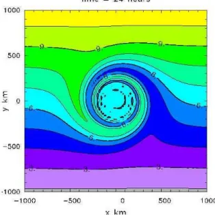
centre and are oriented zonally far from the centre. The pattern after 24 h, shown in Fig. 3.9, illustrates how contours are progressively wound around the vortex with those nearest the centre drawn out into long filaments. This filamentation process is associated with the strong angular shear of the tangential wind profile (see Fig.

3.3b). In reality, the strong gradients of asymmetric relative vorticity would be re- moved by diffusive processes. The filamentation is comparatively slow at larger radial distances so that coherent vorticity asymmetries occur outside the rapidly-rotating and strongly-sheared core. One consequence of these processes is that it is the larger- scale asymmetries that have the main effect on the vortex motion. On account of the filamentation process, there is a natural tendency for vortices to axisymmetrize dis- turbances in their cores. The axisymmetrization process in rapidly-rotating vortices is analyzed in more detail in section 4.1.

The analytic theory described above can be extended to account for higher-order corrections to the vorticity asymmetry. These corrections involve higher-order az- imuthal wavenumber asymmetries. Mathematically an azimuthal wavenumber-n vor- ticity asymmetry has the form

ζ

(r, λ, n) = ζ

(r, t) cos(nλ) + ζ

(r, t) sin(nλ) (n = 1, 2, . . .), which may be written

ζ

(r, λ, n) = ζ

(r, t) cos(nλ + α). (3.26)

Figure 3.8: Approximate trajectories of fluid parcels which, for a given radius, give the maximum asymmetric vorticity contribution at that radius. The figures refer ro the case of motion of an initially-symmetric vortex on a β-plane with zero basic flow at (a) 1 h, (b) 24 h. The particles arc assumed to follow circular paths about the vortex centre (e.g. AB) with angular velocity Ω(r), where Ω decreases monotonically with radius r. Solid lines denote trajectories at 50 km radial intervals. Dashed lines marked ’M’ and ’m’ represent the trajectories giving the overall axisymmetric vorticity maxima and minima, respectively. These maxima and minima occur at the positive and negative ends of the relevant lines.

The associated streamfunction asymmetry has a similar form:

ψ

(r, λ, n) = ψ

(r, t) cos(nλ + α), where(see Appendix 3.4.1)

ψ

= Z

0

dp p

Z

0

sζ

(s, t)ds ψ

= 1

2n

· r

Z

r

p

ζ

(p, t)dp − r

Z

0

p

ζ

(p, t)dp

¸

, (n 6= 0).

The tracks obtained from the extended analytic theory agreed with considerable accuracy with those obtained from a numerical solution of the problem to at least 72 h, showing that theory captures the essential features of the dynamics (see Smith and Weber 1993).

3.3.3 The effects of horizontal shear and deformation

The analytic theory can be extended also to zonal basic flows of the form U =

(U (y, t), 0) (Smith, 1991) and to more general flows with horizontal deformation

Figure 3.9: Analytically calculated absolute vorticity distribution at 24 h correspond- ing with the vorticity asymmetry in the upper right panel of Fig. 3.5.

(Krauss et al. 1995). For simplicity we consider here the case where U is a quadratic function of y only, i.e. U = U

+ U

y +

U

y

. Let us partition the environmental flow at time t into two parts: the initial zonal flow, U, and the part associated with the vortex-induced asymmetries, U

and define the corresponding vorticities:

Γ = k · ∇ ∧ U and ζ

= k · ∇ ∧ U

. Then, noting that U is normal to ∇(Γ + f ), Eq.

(3.6) may be written:

∂ζ

∂t = −u

· ∇(Γ + f ) − (U + U

− c) · ∇ζ

− U

· ∇(Γ + f ). (3.27) Let us define c = U

+ c

, and U = U

(t) + U

, where U

(t) is the speed of the zonal flow at the meridional position of the vortex and U

contains the meridional variation of U, then Eq. (3.27) becomes

∂ζ

∂t = −u

· ∇(Γ + f ) − U

· ∇ζ

+ (U

− c

) · ∇ζ

− U

· ∇(Γ + f). (3.28) The first term on the right-hand-side of this equation represents the asymmetric vorticity tendency, ∂ζ

/∂t, associated with the advection of the absolute vorticity gradient of the basic flow by the symmetric vortex circulation. The second term,

∂ζ

/∂t, is the asymmetric vorticity tendency associated with the basic shear acting

on the symmetric vortex. The third term, ∂ζ

/∂t, is the asymmetric vorticity ten-

dency associated with the advection of symmetric vorticity by the relative asymmet-

ric flow; and the last term, ∂ζ

/∂t, is the asymmetric vorticity tendency associated

with the advection of the absolute vorticity gradient of the basic flow by the asym-

metric flow. Let ζ

(n = 1 . . . 4) be the contribution to ζ

from ∂ζ

/∂t. Then ζ

has an azimuthal wavenumber-1 structure like ζ

in Eq. (3.13) and the solution has the same form as (3.14), but with β replaced with the absolute vorticity gradient of the background flow, β − U

.

Case I: Uniform shear

For a linear velocity profile (i.e. for uniform shear, U

= constant), k·∇Γ = −U

= 0, so that the main difference compared to the calculation in the previous section is the emergence of an azimuthal wavenumber-2 vorticity asymmetry from the term ζ

, which satisfies the equation

∂ζ

∂t = −U

· ∇ζ

= −U

y ∂ζ

∂x .

This result is easy to understand by reference to Figs. 3.10 and 3.11. The vorticity gradient of the symmetric vortex is negative inside a radius of 255 km (say r

) and positive outside this radius (Fig. 3.10). Therefore ∂ζ

/∂x is positive for x > 0 and r > r

and negative for x < 0 and r < r

. If U = U

y, U∂ζ

/∂x is negative in the first and third quadrants for r > r

and positive in the second and fourth quadrants (Figs. 3.11). For r < r

, the signs are reversed.

Figure 3.10: (left) Radial profile of vortex vorticity, ζ(r), corresponding with the tangential wind profile in Fig. 3.3.

Figure 3.12 shows the calculation of ζ

at 24 h when U

= 5 m s

per 1000

km. Since the vorticity tendency is relative to the motion of a rotating air parcel

(Eq. (4.1)), the pattern of ζ

at inner radii is strongly influenced by the large radial

shear of the azimuthal wind and consists of interleaving spiral regions of positive and

negative vorticity. The maximum amplitude of ζ

(1.1 × 10

s

at 24 h) occurs at

a radius greater than r

. Note that azimuthal wavenumber asymmetries other than

wavenumber-1 have zero flow at the origin and therefore have no effect on the vortex

Figure 3.11: Schematic depiction of the azimuthal wavenumber-2 vorticity tendency arising from the term −U · ∇ζ

= −U

y∂ζ

/∂x in the case of a uniform zonal shear U = U

y. (a) shows the sign of the vorticity gradient ∂ζ

/∂x in each quadrant for 0 < r < r

and r

< r where r

is the radius at which the vorticity gradient dζ

/dr changes sign (see Fig. 3.11) and (b) shows the vorticity tendency −U∂ζ

/∂x in the eight regions.

motion. In the case of uniform shear, there is a small wavenumber-1 contribution to the asymmetry from the term ζ

, which satisfies the equation

∂ζ

∂t = −U

· ∇(Γ + f ).

Case II: Linear shear

We consider now the case of a quadratic velocity profile (i.e. linear shear) in which U

is taken to be zero ∂Γ/∂y = −U

is nonzero. Linear shear has two particularly important effects that lead to a wavenumber-1 asymmetry, thereby affecting the vortex track. The first is characterized by the contribution to the absolute-vorticity gradient of the basic flow (the first term on the right-hand-side of Eq. (3.28), which directly affects the zero-order vorticity asymmetry, ζ

. The second is associated with the distortion of the vortex vorticity as depicted in Fig. 3.13 and represented mathematically by ζ

, which originates from the second term on the right-hand-side of Eq. (3.28).

Vortex tracks

Figure 3.14 shows the vortex tracks calculated from the analytic theory of Smith (1991) with the corresponding numerical calculations of Smith and Ulrich (1991).

The broad agreement between the analytical and numerical calculations indicates

Figure 3.12: Asymmetric vorticity contribution for the case of a uniform zonal shear with U

= 5 m s

per 1000 km. Contour interval is 5 × 10

s

. Dashed lines indicate negative values. The vortex centre is marked by a cyclone symbol.

Figure 3.13: Schematic depiction of the wavenumber-1 vorticity tendency arising from the term −U · ∇ζ

= −U∂ζ

/∂x in the case of linear basic shear U = −

U

y

. (a) shows the profile U (y) and (b) shows the vorticity tendency −U∂ζ

/∂x, in the eight regions defined in Fig. 3.10. The sign of ∂ζ

/∂x in these regions is shown in Fig. 3.10a.

that the analytic theory captures the essence of the dynamics involved, even though

the analytically-calculated motion is a little too fast. The eastward or westward displacement in the cases with zonal shear are in accordance with expectations that the vortex is advected by the basic flow and the different meridional displacements are attributed to the wavenumber-1 asymmetry, ζ

discussed above.

Panel (b) of Fig. 3.14 shows a similar comparison for two cases of a linear shear:

SNB with U

= β

and β = 0; SHB U

=

β

and β =

β

; and the case of zero basic flow (ZBF) with β = β

. Here β

is the standard value of β. These three calculations have the same absolute vorticity gradient, β

, but the relative contribution to it from U

and β is different. Note that the poleward displacement is reduced as U

increases in magnitude. Again this effect can be attributed to the wavenumber-one asymmetry ζ

discussed above.

Figure 3.14: Analytically calculated vortex track (denoted by A) compared with

the corresponding numerical solution (denoted by N): (a) uniform shear flow cases

and [b) linear shear flow cases. Each panel includes the analytically and numerically

calculated track for the case of zero basic; flow (denoted ZBF). Cyclone symbols mark

the vortex position at 12-h intervals. (See text for explanation of other letters.)

3.4 Appendices to Chapter 3

3.4.1 Derivation of Eq. 3.16

We require the solution of ∇

ψ

= ζ, when ζ

(r, θ) = ˆ ζ(r)e

. Now

∇

ψ

= ∂

ψ

∂r

+ 1 r

∂ψ

∂r + 1 r

∂

ψ

∂θ

= ˆ ζ(r)e

Put ψ = ˆ ψ(r)e

, then

d

ψ ˆ dr

+ 1

r d ψ ˆ dr − n

r

ψ ˆ = ˆ ζ(r). (3.29)

When ˆ ζ(r) = 0, the equation has solutions ˆ ψ = r

where [α(α − 1) + α − n

]r

= 0, which gives

α

− n

= 0 or α = ±n.

Therefore, for a solution of (3.29), try ˆ ψ = r

φ(r). Then

ψ

= r

φ

+ nr

φ, ψ

= r

φ

+ 2nr

φ

+ n(n − 1)r

φ (3.30) whereupon (3.29) gives

r

φ

+ 2nr

φ

+ n(n − 1)r

φ + r

φ

+ nr

φ − n

r

φ = ˆ ζ, or

r

φ

+ (2n + 1)r

φ

= ˆ ζ.

Multiply by r

and choose β so that n + β = 2n + 1, i.e., β = n + 1. Thus r

is the integrating factor. Then

d dr

£ r

φ(r) ¤

= r

ζ(r), ˆ (3.31)

which may ne integrated to give r

dφ

dr = Z

r

p

ζ(p)dp ˆ + A, where A is a constant. Therefore

dφ

dr = 1 r

Z

r

p

ζ(p)dp ˆ + A

r

Figure 3.15: The domain of integration for the integral (3.32) is the shaded region.

Finally,

φ = Z

r

dq q

Z

q

p

ζ(p)dp ˆ + Z

q

Adq

q

+ B, (3.32) where B is another another constant. The domain of the double integral is the shaded region shown in Fig. 3.15 in which p goes from q to ∞ then q goes from r to ∞. If we change the order of integration in (3.32), q goes from r to p and then p goes from r to ∞, i.e.

φ = Z

r

p

ζ(p)dp Z

r

dq

q

− A

2nr

+ B

= 1

2n

·Z

r

p

ζ(p)dp ˆ − A

¸ 1

r

+ B − 1 2n

Z

0

p

ζ(p)dp. ˆ Finally

ψ(r) = ˆ − r

2n

Z

0

p

ζ(p)dp ˆ + Br

+ 1 2nr

·Z

r

p

ζ(p)dp ˆ − A

¸ .

Now ˆ ψ(r) finite at r = 0 requires that A =

Z

0

p

ζ(p)dp ˆ and ˆ ψ (r) finite as r → ∞ requires that

B = Z

0

p

ζ(p)dp ˆ

Therefore

ψ(r) = ˆ − r

2n

Z

r

p

ζ(p)dp ˆ − r

2n

Z

r

p

ζ(p)dp, ˆ (3.33) as required.

3.4.2 Solution of Eq. 3.25

The asymmetric flow U

is obtained from Eqs. (3.17) and (3.18) and c is obtained from (3.21). We can calculate the streamfunction Ψ

of the vortex-relative flow U

− c, from

ψ

= ψ

− ψ

, where

ψ

= r(V

cos λ − U

sin λ) = r

· ∂ Ψ

∂r

¯ ¯

¯ ¯

r=0

cos λ + ∂Ψ

∂r

¯ ¯

¯ ¯

r=0

sin λ

¸

. (3.34)

Then using (3.15), (3.16), (3.20) and (3.34) we obtain

ψ

= Ψ

(r, t) cos θ + Ψ

(r, t) sin θ, (3.35) where

Ψ

(r, t) = Ψ

− r

· ∂ Ψ

∂r

¸

r=0

, (n = 1, 2)

= 1 2 r

Z

0

µ 1 − p

r

¶

ζ

(p, t)dp. (3.36)

After a little algebra it follows using (3.17), (3.18), (3.21) and (3.36) that

−(U

− c) · ∇ζ

= χ

(r, t) cos θ + χ

(r, t) sin θ, (3.37)

where ·

χ

(r, t) χ

(r, t)

¸

= 1 r

dζ

dr ×

· ψ

(r, t)

−ψ

(r, t)

¸

. (3.38)

Now using (3.37) and (3.38), Eq. (3.36) can be written as dζ

dT = 1 r

dζ

dr (Ψ

(r, t) cos λ − Ψ

(r, t) sin λ) ,

where d/dt denotes integration following a fluid parcel moving in a circular path of radius r about the vortex centre with angular velocity Ω(r). It follows that

ζ

= 1 r

dζ

dr

Z

0

[Ψ

(r, t

) cos λ(t

) − Ψ

(r, t

) sin λ(t

)]dt

,

where λ(t

) = λ − Ω(r)(t − t

). Using Eq. (3.36), this expression becomes ζ

= 1

2 dζ

dr Z

0

Z

0

µ 1 − p

r

¶

× [ζ

(p, t

) cos λ(t

) − ζ

(p, t

) sin λ(t

)] dpdt

, and it reduces further on substitution for ζ

from (3.14) and the above expression for λ(t

) giving

ζ

= 1 2 β dζ

dr Z

0

p µ

1 − p

r

¶

× Z

0

[cos {λ − Ω(r)(t − t

)} − cos {λ − Ω(r)(t − t

) − Ω(p)t

}]dt

dp.

On integration with respect to t

we obtain

ζ

(r, θ, t) = ζ

(r, t) cos λ + ζ

(r, t) sin λ (3.39) where

ζ

(r, t) = Z

0

χ

(r, t)dt

= − 1 2 β dζ

dr Z

0

p µ

1 − p

r

¶

η

(r, p, t)dp, (3.40) and

η

(r, p, t) = sin {Ω(r)t}

Ω(r) − sin {Ω(r)t} − sin {Ω(p)t}

Ω(r) − Ω(p) , (3.41)

η

(r, p, t) = 1 − cos {Ω(r)t}

Ω(r) + cos {Ω(r)t} − cos {Ω(p)t}

Ω(r) − Ω(p) , (3.42)

The integrals in (3.41) can be readily evaluated using quadrature.