Class notes for Nonlinear ODEs and dynamical systems Hamiltonian dynamics
Henk Bruin June 11, 2021
Hamiltonian Dynamics
In general coordinates (p, q) ∈ R2n, q = position, p = momentum (usually), the Hamiltonian equations are:
q˙
˙ p
=XH q
p
= ∂H
∂p
−∂H∂q
=
∇pH
−∇qH
| {z }
in vector notation
for the Hamiltonian function H :R2n →R. Throughout we assume that H isC2-smooth. The H is preserved along orbits:
H˙ =∇qH•q˙+∇pH•q˙=∇qH• ∇qH+∇pH•(−∇qH) = 0.
(Here •stands for the usual dot-product.) UsuallyH represent the energy, but other preserved quantities (e.g. momentum or angular momentum) are possible too.
Theorem 1. The Hamiltonian flow φtH preserves volume in R2n.
This “volume” is sometimes calledLiouville measure in this context.
Proof. Let Ω ⊂R2n be some region in R2, and V(t) = Vol(φtH(Ω)) its volume after flowing for time t. In other words
V(t) = Z
φtH(Ω)
dVol.
A standard result in multivariate calculus (see Theorem 14 Schmeiser’s Notes) says that V˙(t) =
Z
φtH(Ω)
divXHdVol, where the divergence is defined as
divXH =
n
X
i=1
∂
∂qi(XH)pi +
n
X
i=1
∂
∂pi(XH)pi
=
n
X
i=1
∂
∂qi( ∂
∂piH) +
n
X
i=1
∂
∂pi(− ∂
∂qiH) = 0.
Therefore ˙V(t) = 0 and V(t) is constant as claimed.
Lagrangian Dynamics
In general coordinates (v, q)∈R2n, q= position, v = ˙q = velocity (usually), the Lagrangian is L:R2 →R. We assume that Lis C2-smooth.
The task is to find an extremum of the action of the Lagrangian over all C1-paths, i.e., minimize
I({( ˙q(t), q(t)) :t1 ≤t≤t2}) = Z t2
t1
L( ˙q(t), q(t)) dt,
where q(t1), q(t2) are both fixed.
Figure 1: The path q(t) and its perturbation b(t) =εr(t)
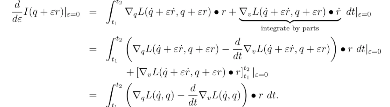
For a perturbation path{r(t) :t1 ≤t≤ t2} with r(t1) =r(t2) = 0 (see Figure 1), compute the Gateaux derivative:
d
dεI(q+εr)|ε=0 = Z t2
t1
∇qL( ˙q+εr, q˙ +εr)•r+∇vL( ˙q+εr, q˙ +εr)•r˙
| {z }
integrate by parts
dt|ε=0
= Z t2
t1
∇qL( ˙q+εr, q˙ +εr)− d
dt∇vL( ˙q+εr, q˙ +εr)
•r dt|ε=0 + [∇vL( ˙q+εr, q˙ +εr)•r]tt2
1|ε=0
= Z t2
t1
∇qL( ˙q, q)− d
dt∇vL( ˙q, q)
•r dt.
The constant terms in the penultimate line above disappear becauser(t1) =r(t2) = 0. In order to have dεdI(q+εr)|ε=0= 0 over all paths r, we need
∇qL( ˙q, q) = d
dt∇vL( ˙q, q). (1)
These are the Euler-Lagrange equations (one for every coordinate ofq).
The Legendre Transforms
Letf : domain of f =U ⊂Rn →R be a C2-smooth strictly convex function. This means that
D2f =
∂2f
∂x21 . . . ∂x∂2f
1∂xn
... ...
∂2f
∂xn∂x1 . . . ∂x∂2f2 n
is a positive definite matrix: (D2f)v•v >0 unless v = 0.
Define theLegendre transform
f∗(v) = sup
v∈U
p•v−f(v). (2)
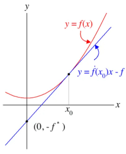
The supremum f∗(p) corresponds to the infimum of −f∗(p), and this is the intersection of the vertical axis with lines of slope p intersecting the graph of f, see Figure 2. This infimum is achieved when this line of slope pis tangent to the graph.
Figure 2: Illustration of the Legendre transform with x=v, p= ˙f(v) and x0 =v∗. Letv∗(p) be the value where the supremum is assumed (so (v∗(p), f(v∗(p))) is the point of tangency). Then
p = ∇vf(v∗(p)), (3)
f∗(p) = p•v∗(p)−f(v∗(p)). (by inserting (3) in (2)) (4) Theorem 2. Let f be strictly convex C2 function. Then
• f∗ is a strictly convex C2 function;
• f∗∗=f.
Proof. Compute
∇pf∗(p) =
|{z}
by (4)
∇p(p•v∗(p))−f(v∗(p)))
= v∗(p) + p• ∇pv∗(p)
| {z }
p=∇vf(v∗(p)) by (3)
−∇vf(v∗(p))• ∇pv∗(p)
= v∗(p).
so (3) holds with f∗ instead of f and the roles of v and p swapped. But then (4) follows as well. So f∗∗=f.
In fact, we also have ∇pf∗(p) =v,∇vf(v) = p, so
∇vf = (∇pf∗)inv (5) Now f isC2 strictly convex
⇔ the Jacobian matrix D2f =J(∇f) is positive definite
⇔ J(∇f)−1 is positive definite
⇔ (by (5)) J(∇f∗) = D2f∗ is positive definite
⇔ f∗ isC2 strictly convex.
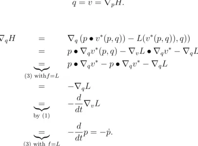
Theorem 3. Assume that (for each q fixed) the Hamiltonian is the Legendre transform of the Lagrangian, so by (3) and (4)
p=∇vL(v∗, q) and H(p, q) =L∗(v, q) = p•v∗(p)−L(v∗(p)), q).
Then the Euler-Lagrange equations are equivalent to the Hamiltonian equations.
Proof. We assumed H = L∗ so by the previous theorem also L = H∗. Using (3) with f = H and v and pswapped, we find the first Hamiltonian equation:
˙
q=v =∇pH.
Also, by (4)
∇qH = ∇q(p•v∗(p, q))−L(v∗(p, q)), q))
= p• ∇qv∗(p, q)− ∇vL• ∇qv∗ − ∇qL
=
|{z}
(3) withf=L
p• ∇qv∗−p• ∇qv∗− ∇qL
= −∇qL
=
|{z}
by (1)
−d dt∇vL
=
|{z}
(3) withf=L
−d
dtp=−p.˙ This is the second Hamiltonian equation.
The example of the pendulum
Newton’s equation of motion for the pendulum (see Figure 3) is:
¨ q+ g
` sinq = 0, (6)
for the angle q.
Figure 3: The pendulum with gravitational force along the rod F =−mgsinq In the Hamiltonian setting, we set p=m`2q,˙
Ekin = m(`q)˙ 2
2 = p2
2m`2, Epot =−mg`cosq, and Hamiltonian
H(p, q) =Ekin+Epot = p2
2m`2 −mg`cosq.
Then
∂H
∂p = m`p2 = ˙q
−∂H∂q =−mg`sinq =
|{z}
Newton’s eq. of motion
`2mq¨= ˙p.
From Lagrangian point of view with v = ˙q:
Lagrangian =L(v, q) = Ekin−Epot = m`2v2
2 +mg`cosq.
The Euler-Lagrangian equation gives 0 =∇qL− d
dt∇vL=−mg`sinq− d dtm`2q˙
⇔ 0 = g
` sinq+ ¨q, which is Newton’s equation of motion.
Now we compare the Hamiltonian and Lagrangian using the Legendre transform. Start with v = ˙q and L(v, q) = m`22v2 +mg`cosq. Take the Legendre transform to get the Hamiltonian:
H(p, q) = sup
v∈R
p•v−
m`2v2
2m +mg`cosq
.
Set the derivative dvd = 0: p−m`2v = 0, so v = m`p2. (Thus p=m`2v =m`q˙ – this somewhat strange form of the momentum is a result of Legendre transforming a somewhat strange form of velocity, which is really an angular velocity of physical dimension [1/sec]). Insert
H(p, q) = p2
m`2 − m`2p2
2m2`4 −mg`cosq
= p2
2m`2 −mg`cosq
= Ekin+Epot. Relativistic pendulum
In order to illustrate that the relation between Lagangian and Hamiltonian can be more com- plicated than just flipping the sign of the potential energy, we consider the pendulum within the framework of Einstein’s relativistic mechanics.
(
Ekin=m(v)c2, m(v) = m0 q
1 + |v|c22. Epot=Epot(q).
Herecis the speed of light, v the velocity andm0 the rest-mass of the particle. Note that v = ˙q is a vector, and |v|=pP
ivi2.
The Lagrangian is defined asL(v, q) =Ekin−Epot, and therefore
∂
∂viL(v, q) = m0c2 2
q
1 + |v|c22
2vi
c2 = m0vic pc2+|v|2. Therefore the Euler-Lagrange equations become
∇qEpot(q) = d dt
m0cq˙ pc2+|q|˙2.
We find the Hamiltonian via the Legendre transform:
H(p, q) = L∗(v, q) = sup
v∈Rn
v•p− m0c2 r
1 + |v|2
c2 −Epot(q)
!
. (7)
Solve ∇vL(v, q) = 0:
p= m0cv
pc2+|v|2 ⇒ |v|2 = c2|p|2 m20c2− |p|2.
Insert in (7)
H(p, q) = c|p|2
pm20c2 − |p|2 −m0c2 s
1 + |p|2
m20c2− |p|2 +Epot(q)
= −c q
m20c2− |p|2+Epot(q).
Noether’s Theorem and First Integrals
Not only energy can supply the Hamiltonian; there are often other preserved (additional) quantities, e.g. momentum, angular momentum. Such constants of motion are called first integrals. These can often be related to a continuous symmetry in the system. This is the content of Noether’s Theorem.
LetQ(s, q) be a continuous family of motions in Rn. For instance, rotations in R2 over an angle s:
Q: (s, q)7→
coss −sins sins coss
q1 q2 .
Formally, Q(0, q) =q and Q(s+t, q) =Q(s, Q(t, q)) for all q ∈Rn and s, t ∈R. Therefore we can describe Q(s, q) as the solution of a flow of a vector field, sayf :Rn→Rn:
(∂
∂sQ(s, q) =f(Q(s, q)),
Q(0, q) = q. (8)
The corresponding action on tangent vectors v = ˙q ∈TqRn (which is isomorphic to Rn) is v 7→DqQ(s, q)v,
with s-derivative ats = 0:
∂
∂sDqQ(s, q)|s=0 =Dq ∂
∂sQ(s, q)|s=0 =Dqf(Q(s, q))|s=0 =Dqf(q). (9) Definition 4. A vector field f (with ∂s∂(Q(s, q)) = f(Q(s, q))) generates a symmetry of a Lagrangian system if
L(v, q) =L(DqQ(s, q)v, Q(s, q)) (10) for all s∈R andq ∈Rn, v ∈TqRn. That is,L remains constant over actions of the symmetry.
Theorem 5 (Noether’s Theorem). If f generates a symmetry, then I(v, q) :=∇vL(v, q)•f(q)
is a first integral.
Proof. Differentiate (10) with respect to s at s = 0. Because L is constant over the action of Q(s, q), we obtain
0 = d
dsL(DqQ(s, q)v, Q(s, q))|s=0
= ∇vL• d
dsDqQ(s, q)v +∇qL• d
dsQ(s, q)
| {z }
=f(q)
|s=0 (11)
Hence
I(v, q)˙ = d
dt∇vL(v, q)•f+∇vL(v, q)•
∇qf• d dtq
|{z}v
| {z }
d
dsDqQ(s,q)v|s=0by (9)
=
|{z}
by (11)
d
dt∇vL•f(q)− ∇qL•f(q)
=
|{z}
by (1)
d
dt∇vL− ∇qL
•f(q) = 0.
Hence I is constant as claimed.
Examples: Assume that q ∈ Rn and L(v, q) = Ekin(v)−Epot(q) (with Ekin = mv22) does not depend on the coordinateqj. TakeQ(s, q) =q+sej, soQ(0, q) =q and the corresponding vector field is
f(q) = ej the j-th basis vector in Rn. Then
I(v, q) = ∇vL(v, q)•f(q)
= ∇v(Ekin(v)−Epot(q))•f(q)
= mv•ej =mvj =pj
is the j-th component of the momentum. That is: the j-th component of the momentum is preserved.
For rotational symmetries q 7→ Q(s, q) = A(s)q for a family of skew-symmetric matrices, e.g., A(s) =
coss −sins sins coss
, the preservation of
I(v, q) =mvTA(0)q.
leads to the preservation of (a component of) the angular momentum.
Definition 6. When a Hamiltonian system in R2n has n first integrals Ij, j = 1, . . . , n, then the system is called integrable. This doesn’t mean that you can solve the system explicitly (in general), but that trajectories are confined to the intersection of level sets
n
\
j=1
{(v, q) :Ij(v, q) =aj}.
When these level sets are compact, they are almost surely (i.e., for almost all values aj) n- dimensional tori.
Figure 4: Parallel flow on the torus and on nested tori.
As an example, note that constant parallel motion
˙ x=C~
on a d-dimensional torus is dense in a d−i-dimensional torus if the d coordinates of C~ have i rational relations among them. For instance, if C~ = (c1, c2)T, then the motion is periodic if ac1 =bc2 for some (a, b)∈Z2\ {(0,0)}, and dense fills the 2-dimensional torus if not.
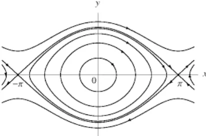
Figure 5: The phase portrait of the pendulum.
A second example is the pendulum, with n = 1 and H = Ekin +Epot a first integral.
Therefore this system is integrable. In Figure 5, if we take x = q mod 2π ∈ [−π, π], then all orbits are compact in the cylinder. All the orbits are topological circles, except the two equilibria at (0,0) and (±π,0).
0.1 The n-body problem
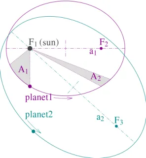
The 2-body problem (Kepler’s Problem) is about the motio of two particles (e.g. the Sun and the Earth) moving in ech other’s gravitational field in R3, and no other forces around. Kepler, as well known in science history, gave three laws to describe the motion of the planets:
1. The orbit of a planet is an ellipse with the Sun at one of the two foci.
2. A line segment joining a planet and the Sun sweeps out equal areas during equal intervals of time:
3. The square of the orbital period T of a planet is directly proportional to the cube of the semi-major axis a of its orbit:
T2 ∼a3.
Figure 6: Illustration of Kepler’s Laws.
Here the dimension of the problem is n = 6 (3 space coordinates ~qS of the Sun, 3 space coordinates ~qE of the Earth), and there are (more than) 6 first integrals:
• the momentum vector p∗ = p~S +~pE (3 components), where ~pS = mSdtd~qS and ~pE = mEd
dt~qE;
• the angular momentum vector `∗ = ~pS×~qS +~pE ×~qE. (This is equivalent to Kepler’s second law).
Therefore all bounded motions are confined to a 6-dimensional torus (integrable).
There are, however, more first integrals, each of them reducing the dimension in which orbits
• From the Galilei transformations (~v, ~q)7→(~v−~v0, ~q−t~v0) (which allows us to putp∗ = 0).
• Energy Ekin+Epot.
• The Laplace-Runge-Lenz vector p∗ ×`∗ −α|~~qq|, where the constant α is depends on the masses of Sun and Earth an don the gravitational constantGin Newton law of attraction:
Fgrav =GmSmE
r2 . G≈6.67410−11 m3
kg.sec2. (12)
This first integral exists precisely because the gravitation force is inverse square propor- tional to the mutual distance between Sun and Earth.
This reduces the orbits to 1-dimensional tori, i.e., ellipses, as Kepler’s first law states (or to hyperbolas or parabolas if the orbit is not compact). In fact, also Kepler’s third law is a consequence of the preservation of the Laplace-Runge-Lenz vector (so again of the precise form of the Newtonian gravitation).
Let us try to derive the elliptical motion (i.e., solve Kepler’s problem) with a bit of physical insight:
mS~qS+mE~qE = 0 the center of mass fixed at the origin;
p∗ =mS~vS+mE~vE = 0 preservation of momentum;
`∗ =~pS×~qS+~pE×~qE =c~e3 preservation of angular momentum,
we choose coordinates to keep orbits inx, y-plane.
Use polar coordinates for
~r:=~qS −~qE =rcosφ ~e1+rsinφ ~e2. r =|~r|.
Since the origin is the center of mass, we have
~
qS = mE mE +mS
~r, ~qE =− mS mE+mS
~ r.
Now we compute the angular momenta of Sun and Earth explicitly:
`S = mS mE mS +mE
d
dt(rcosφ)
d
dt(rsinφ) 0
× mE mS+mE
rcosφ rsinφ
0
= mS
mE mS+mE
2
˙
rcosφ−rφ˙sinφ
˙
rsinφ+rφ˙sinφ 0
×
rcosφ rsinφ
0
= mS
mE
mS+mE 2
0 0 r2φ˙
. Similarly
`E =mE
mS mS+mE
2
0 0 r2φ˙
. Thus
|`∗|:=|`S|+|`E|=m∗r2φ,˙ m∗ = mSmE
mS +mE. (13)
Next we compute the kinetic energies of Sun and Earth explicitly:
Ekin,S = mS|~vS|2
2 = mS 2
d
dt(rcosφ)
d
dt(rsinφ) 0
2
= mS 2
mE mS+mE
2
( ˙r2+r2φ˙2), and similarly
Ekin,E = mE 2
mS mS+mE
2
( ˙r2+r2φ˙2).
Their combined potential energies are
Epot =−mSmEG r . Adding all the energies together:
E = m∗
2 ( ˙r2+r2φ˙2)− mSmEG
r . (14)
Solve r as function of φ, using (13) (i.e., |`∗|=m∗r2φ):˙
˙ r= dr
dφ dφ
dt = dr dφ
φ˙ =−dr dφ
|`∗| m∗r2. Inserted in (14):
E = |`∗|2 2m∗
1 r4
dr dφ
2
+ 1 r2
!
− mSmEG r .
We can simplify this differential equation by taking r = 1ρ, so drdφ =−ρ12
dρ
dφ. This gives E = |`∗|2
2m∗
dρ dφ
2
+ρ2
!
−mSmEG ρ.
Next split off the square:
dρ dφ
2
+ (ρ−A)2 =B2,
(A= m∗m|`S∗|m2EG, B =A2+ 2m|`∗∗|E. Introduce a new variable ψ by setting ρ=A+Bcosψ:
B2sin2ψ dψ
dφ 2
+B2cos2ψ =B2 ⇒
dψ dφ
2
= 1.
We choose the positive solution dψdφ = 1 (the negative solution will result in the same shape of orbit, traversed in the opposite direction). Therefore
ψ =ψ(φ) = φ−φ0, ρ(φ) = A+Bcos(φ−φ0), and
r(φ) = A−1
1 +εcos(φ−φ0) with eccentricity ε = B A =
s
1 + 2E|`∗| m∗(mSmE)2G. In Cartesian coordinates x=r(φ) cos(φ−φ0),y=r(φ) sin(φ−φ0), this is
(1−ε2)x2+y2 = r2 (1−ε2) cos2(φ−φ0) + sin2(φ−φ0)
= A−2
(1 +εcos(φ−φ0))2 1−ε2cos2(φ−φ0)
= 1
A2
1−εcos(φ−φ0) 1 +εcos(φ−φ0)
= 1
A2
1 +εcos(φ−φ0)−2εcos(φ−φ0) (1 +εcos(φ−φ0)) = 1
A2 −2εx A .
which gives
(1−ε2)x2+2εx
A +y2 =A2. Finally, for the eccentricity we have:
ε
<1 if E <0 and we have an ellipse,
= 1 if E = 0 and we have a parabola,
>1 if E >0 and we have a hyperbola.
Figure 7: Paris mathematicians with an L, in alphabetical and chronological order.
The mathematical explanation (in first place due to Newton) for Kepler’s Laws was a big triumph of the use of mathematics to understand the world. In the wake of the Enlightening (Aufkl¨arung) philosophical movement of the late 17th century, it gave ground for an optimistic view on determinism, i.e., the view that in nature everything is predictable. This was most famously expressed by Laplace:
We may regard the present state of the universe as the effect of its past and the cause of its future. An intellect1 which at a certain moment would know all forces that set nature in motion, and all positions of all items of which nature is composed, if this intellect were also vast enough to submit these data to analysis, it would embrace in a single formula the movements of the greatest bodies of the universe and those of the tiniest atom; for such an intellect nothing would be uncertain and the future just like the past would be present before its eyes. 2
However, the three body problem, and more generally the eight body problem (i.e., the Solar system, Neptune was discovered in 1848, making it a nine body problem, Pluto was only discovered in 1930) stubbornly refused to be integrable, at least all the efforts of 19th century mathematics went in vain. As such, it remained an open question whether the planets would circle around the Sun for ever, or actually have unstable orbits, maybe swinging off to outer space, or colliding with one another at some point in the future. The Swedish mathematician Mittag-Leffler persuaded King Oscar II to arrange an international prize competition in math- ematics honouring the king’s 60th birthday in 1884. This competition was won by the French
1also called: Laplace’s demon
2Pierre Simon Laplace, A Philosophical Essay on Probabilities
mathematician Henri Poincar´e with a lengthy essay3 which can be seen as the beginning of
“Dynamical Systems”, and in which he showed that predicting motions as complicated as the three body problem can, in general and to any degree of accuracy and in spite of “determinism”, not be accomplished. The reason is the occurrence of sensitive dependence on initial conditions and of horseshoes, but the words for these notions emerge much later.
Modern computer simulations confirm that there is no way of saying whether, for instance, the Earth and Mars will collide within the next 50 million years or not. Computers also found some very unexpected periodic orbits (choreographies) for three or more bodies, see Figure 8.
Figure 8: Some possible periodic orbits for three (and even six) bodies.
Exercise 7. Show that if the Hamiltonian H = Ekin(p) +Epot(q) and Ekin = 2mp2 , then the Lagrangian is L=Ekin(p)−Epot(q).
Exercise 8. Given is the differential equation
˙
x=C, x∈T2 =R2/Z2, C = c1
c2
∈R2.
Show that:
• the return map F : S1 → S1 of the flow ϕt to the circle S1 = {x ∈ T2 : x1 = 0} is a rotation over c1/c2.
• hence all orbits of F are dense if and only if c1/c2 ∈/ Q.
• hence all orbit of ϕt are dense if and only if c1/c2 ∈/ Q.
What does this say about the Poincar´e-Bendixson theorem on the torus T2? Exercise 9. Assume that XH is a Hamiltonian vector field in R2:
• Show that equilibria of XH can only be centers or saddles.
• Which bifurcations (of the ones we treated in class) can occur in a family of Hamiltonian vector fields?
• Find a family of Hamiltonians Hε :R2 →R such that atε= 0, a saddle becomes a center.
Exercise 10. A Lagrangian system in R3 has the Lagrangian
L(v, q) = v21 +v22+v32
2 − q21+q22+q33
2 .
Use Noether’s Theorem to find first integrals. Is the system integrable?
3Poincar´e discovered a mistake in the first version of his essay, corrected it, and had to spend all his prize money to recall the wrong first version that was already in print.
Exercise 11. We have a Hamiltonian system in coordinates (x, y)∈R2 where the Hamiltonian has the form
H(x, y) = y2
2 +V(x), V isC2-smooth, and assume that V(x) =V(−x) has V00(0) >0. This means that (0,0) is
(a) Show that (0,0) is a center, with periodic motion around it.
(b) Let T(a) be the period of the orbit starting at (a,0). Show that T(a) =
Z a 0
4
p2(V(a)−V(x))dx.
Hint: Integrate T(a) =Rt2
t1 a quarter of the periodic orbit and invert t=t(x) (instead of x=x(t)) to rewrite the integral.
• Show that T(a) = 2π is constant forV(x) = x22 (harmonic oscillator).
• Show that T(a) is increasing if V(x) = −cosx (pendulum), and find lima&0T(a) and lima%0T(a).
Solution to Exercise 9: By Liouville’s Theorem, the Hamiltonian flow preserves area, so there cannot be sinks or saddles (because locally these contract resp. expand area). As such, fold bifurctions and Hopf bifurcations cannot occur, neither pitchfork bifurcations. However, for the Hamiltonian H(x, y) = y22 +εx2+x4, the center at (0,0) turns into saddle asε becomes negative. The eigenvalues of this equilibrium, which are two purely imaginary complex conju- gates, first decrease to 0, and then become real (one postive, the other negative).
Solution to Exercise 11: (a) Equilibria at (x,0) where V0(x) = 0, and DXH(x,0) = 0 1
−V00(x) 0
. Since V00(0) > 0, the eigenvalues are λ± = ±p
V00(0)i, so purely imaginary, and therefore 0 is a center.
(b) Let t1 and t2 be the points in time where the orbit through (a,0) hits the positive vertical resp. positive horizontal axis. We have, by change of coordinates x=x(t).
T(a) = 4 Z t2
t1
dt= Z a
0
dt dx dx=
Z a 0
1 y dx.
We compute y from H = y22 +V(x), so y = p
2(H−V(x)). But H(x, y) = H(y,0) = V(a) because it is a constant of motion. Therefore
T(a) = 4 Z a
0
1
p2(V(a)−V(0)) dx.
(c) Take V(x) = x22. Then, using x=asinψ, T(a) = 4
Z a 0
√ 1
a2−x2 dx= 4 Z π2
0
asinψ
pa2(1−sinψ2) dψ= 4 Z π2
0
dψ= 2π.
(d) For V(x) =−cosx we have T(a) = 4Ra 0
√ 1
2(cos(x)−cos(a)) dx. This integral cannot be solved with an explicit expression, ut for 0≤x≤a both small, we can use the Taylor expansion:
lima→0T(a) = lim
a→04 Z a
0
1 q
2(1−x22 −(1− a22))
dx= lim
a→04 Z a
0
√ 1
a2−x2 dx= 2π as in (c). For a→π/2, we simply plug in the value:
a→limπ
2
T(a) = 4 Z π2
0
√ 1
cosx dx = 4 Z π2
0
cosx (cosx)3/2 dx.
Change coordinates u= sinx and then v = 1−u:
lim
a→π2 T(a) = 4 Z 1
0
du
(1−u2)3/2 = 4 Z 1
0
v−3/2(2−v)−3/2dv≥√ 2
Z 1 0
v−3/2dv=∞.