EUROPEAN ORGANIZATION FOR NUCLEAR RESEARCH

arXiv:hep-ex/0007040v1 20 Jul 2000

EUROPEAN ORGANIZATION FOR NUCLEAR RESEARCH

CERN-EP-2000-092 July 7, 2000

Two Higgs Doublet Model and Model Independent Interpretation of Neutral Higgs Boson Searches

The OPAL Collaboration

Abstract

Searches for the neutral Higgs bosons h ⁰ and A ⁰ are used to obtain limits on the Type II Two Higgs Doublet Model (2HDM(II)) with no CP–violation in the Higgs sector and no additional particles besides the five Higgs bosons. The analysis combines approximately 170 pb ⁻¹ of data collected with the OPAL detector at √

s ≈ 189 GeV with previous runs at √

s ≈ m Z and √

s ≈ 183 GeV. The searches are sensitive to the h ⁰ , A ⁰ → q¯q, gg, τ ⁺ τ ⁻ and h ⁰ → A ⁰ A ⁰ decay modes of the Higgs bosons. For the first time, the 2HDM(II) parameter space is explored in a detailed scan, and new flavour independent analyses are applied to examine regions in which the neutral Higgs bosons decay predominantly into light quarks or gluons. Model–independent limits are also given.

(Submitted to European Physical Journal C)

The OPAL Collaboration

G. Abbiendi ² , K. Ackerstaff ⁸ , C. Ainsley ⁵ , P.F. ˚ Akesson ³ , G. Alexander ²² , J. Allison ¹⁶ , K.J. Anderson ⁹ , S. Arcelli ¹⁷ , S. Asai ²³ , S.F. Ashby ¹ , D. Axen ²⁷ , G. Azuelos ^18,a , I. Bailey ²⁶ ,

A.H. Ball ⁸ , E. Barberio ⁸ , R.J. Barlow ¹⁶ , S. Baumann ³ , T. Behnke ²⁵ , K.W. Bell ²⁰ , G. Bella ²² , A. Bellerive ⁹ , G. Benelli ² , S. Bentvelsen ⁸ , S. Bethke ³² , O. Biebel ³² , I.J. Bloodworth ¹ , O. Boeriu ¹⁰ , P. Bock ¹¹ , J. B¨ohme ^14,h , D. Bonacorsi ² , M. Boutemeur ³¹ ,

S. Braibant ⁸ , P. Bright-Thomas ¹ , L. Brigliadori ² , R.M. Brown ²⁰ , H.J. Burckhart ⁸ , J. Cammin ³ , P. Capiluppi ² , R.K. Carnegie ⁶ , A.A. Carter ¹³ , J.R. Carter ⁵ , C.Y. Chang ¹⁷ ,

D.G. Charlton ^1,b , P.E.L. Clarke ¹⁵ , E. Clay ¹⁵ , I. Cohen ²² , O.C. Cooke ⁸ , J. Couchman ¹⁵ , C. Couyoumtzelis ¹³ , R.L. Coxe ⁹ , A. Csilling ^15,j , M. Cuffiani ² , S. Dado ²¹ , G.M. Dallavalle ² ,

S. Dallison ¹⁶ , A. de Roeck ⁸ , E. de Wolf ⁸ , P. Dervan ¹⁵ , K. Desch ²⁵ , B. Dienes ^30,h , M.S. Dixit ⁷ , M. Donkers ⁶ , J. Dubbert ³¹ , E. Duchovni ²⁴ , G. Duckeck ³¹ , I.P. Duerdoth ¹⁶ , P.G. Estabrooks ⁶ , E. Etzion ²² , F. Fabbri ² , M. Fanti ² , L. Feld ¹⁰ , P. Ferrari ¹² , F. Fiedler ⁸ ,

I. Fleck ¹⁰ , M. Ford ⁵ , A. Frey ⁸ , A. F¨ urtjes ⁸ , D.I. Futyan ¹⁶ , P. Gagnon ¹² , J.W. Gary ⁴ , G. Gaycken ²⁵ , C. Geich-Gimbel ³ , G. Giacomelli ² , P. Giacomelli ⁸ , D. Glenzinski ⁹ , J. Goldberg ²¹ , C. Grandi ² , K. Graham ²⁶ , E. Gross ²⁴ , J. Grunhaus ²² , M. Gruw´e ²⁵ , P.O. G¨ unther ³ , C. Hajdu ²⁹ , G.G. Hanson ¹² , M. Hansroul ⁸ , M. Hapke ¹³ , K. Harder ²⁵ , A. Harel ²¹ , M. Harin-Dirac ⁴ , A. Hauke ³ , M. Hauschild ⁸ , C.M. Hawkes ¹ , R. Hawkings ⁸ ,

R.J. Hemingway ⁶ , C. Hensel ²⁵ , G. Herten ¹⁰ , R.D. Heuer ²⁵ , J.C. Hill ⁵ , A. Hocker ⁹ , K. Hoffman ⁸ , R.J. Homer ¹ , A.K. Honma ⁸ , D. Horv´ath ^29,c , K.R. Hossain ²⁸ , R. Howard ²⁷ , P. H¨ untemeyer ²⁵ , P. Igo-Kemenes ¹¹ , K. Ishii ²³ , F.R. Jacob ²⁰ , A. Jawahery ¹⁷ , H. Jeremie ¹⁸ ,

C.R. Jones ⁵ , P. Jovanovic ¹ , T.R. Junk ⁶ , N. Kanaya ²³ , J. Kanzaki ²³ , G. Karapetian ¹⁸ , D. Karlen ⁶ , V. Kartvelishvili ¹⁶ , K. Kawagoe ²³ , T. Kawamoto ²³ , R.K. Keeler ²⁶ , R.G. Kellogg ¹⁷ , B.W. Kennedy ²⁰ , D.H. Kim ¹⁹ , K. Klein ¹¹ , A. Klier ²⁴ , S. Kluth ³² , T. Kobayashi ²³ , M. Kobel ³ , T.P. Kokott ³ , S. Komamiya ²³ , R.V. Kowalewski ²⁶ , T. Kress ⁴ ,

P. Krieger ⁶ , J. von Krogh ¹¹ , T. Kuhl ³ , M. Kupper ²⁴ , P. Kyberd ¹³ , G.D. Lafferty ¹⁶ , H. Landsman ²¹ , D. Lanske ¹⁴ , I. Lawson ²⁶ , J.G. Layter ⁴ , A. Leins ³¹ , D. Lellouch ²⁴ , J. Letts ¹² , L. Levinson ²⁴ , R. Liebisch ¹¹ , J. Lillich ¹⁰ , B. List ⁸ , C. Littlewood ⁵ , A.W. Lloyd ¹ ,

S.L. Lloyd ¹³ , F.K. Loebinger ¹⁶ , G.D. Long ²⁶ , M.J. Losty ⁷ , J. Lu ²⁷ , J. Ludwig ¹⁰ , A. Macchiolo ¹⁸ , A. Macpherson ^28,m , W. Mader ³ , S. Marcellini ² , T.E. Marchant ¹⁶ ,

A.J. Martin ¹³ , J.P. Martin ¹⁸ , G. Martinez ¹⁷ , T. Mashimo ²³ , P. M¨attig ²⁴ , W.J. McDonald ²⁸ , J. McKenna ²⁷ , T.J. McMahon ¹ , R.A. McPherson ²⁶ , F. Meijers ⁸ , P. Mendez-Lorenzo ³¹ , W. Menges ²⁵ , F.S. Merritt ⁹ , H. Mes ⁷ , A. Michelini ² , S. Mihara ²³ ,

G. Mikenberg ²⁴ , D.J. Miller ¹⁵ , W. Mohr ¹⁰ , A. Montanari ² , T. Mori ²³ , K. Nagai ⁸ , I. Nakamura ²³ , H.A. Neal ^12,f , R. Nisius ⁸ , S.W. O’Neale ¹ , F.G. Oakham ⁷ , F. Odorici ² , H.O. Ogren ¹² , A. Oh ⁸ , A. Okpara ¹¹ , M.J. Oreglia ⁹ , S. Orito ²³ , G. P´asztor ^8,j , J.R. Pater ¹⁶ ,

G.N. Patrick ²⁰ , J. Patt ¹⁰ , P. Pfeifenschneider ^14,i , J.E. Pilcher ⁹ , J. Pinfold ²⁸ , D.E. Plane ⁸ , B. Poli ² , J. Polok ⁸ , O. Pooth ⁸ , M. Przybycie´ n ^8,d , A. Quadt ⁸ , C. Rembser ⁸ , P. Renkel ²⁴ , H. Rick ⁴ , N. Rodning ²⁸ , J.M. Roney ²⁶ , S. Rosati ³ , K. Roscoe ¹⁶ , A.M. Rossi ² , Y. Rozen ²¹ ,

K. Runge ¹⁰ , O. Runolfsson ⁸ , D.R. Rust ¹² , K. Sachs ⁶ , T. Saeki ²³ , O. Sahr ³¹ , E.K.G. Sarkisyan ²² , C. Sbarra ²⁶ , A.D. Schaile ³¹ , O. Schaile ³¹ , P. Scharff-Hansen ⁸ , M. Schr¨oder ⁸ , M. Schumacher ²⁵ , C. Schwick ⁸ , W.G. Scott ²⁰ , R. Seuster ^14,h , T.G. Shears ^8,k ,

B.C. Shen ⁴ , C.H. Shepherd-Themistocleous ⁵ , P. Sherwood ¹⁵ , G.P. Siroli ² , A. Skuja ¹⁷ ,

A.M. Smith ⁸ , G.A. Snow ¹⁷ , R. Sobie ²⁶ , S. S¨oldner-Rembold ^10,e , S. Spagnolo ²⁰ ,

M. Sproston ²⁰ , A. Stahl ³ , K. Stephens ¹⁶ , K. Stoll ¹⁰ , D. Strom ¹⁹ , R. Str¨ohmer ³¹ ,

L. Stumpf ²⁶ , B. Surrow ⁸ , S.D. Talbot ¹ , S. Tarem ²¹ , R.J. Taylor ¹⁵ , R. Teuscher ⁹ ,

M. Thiergen ¹⁰ , J. Thomas ¹⁵ , M.A. Thomson ⁸ , E. Torrence ⁹ , S. Towers ⁶ , D. Toya ²³ , T. Trefzger ³¹ , I. Trigger ⁸ , Z. Tr´ocs´anyi ^30,g , E. Tsur ²² , M.F. Turner-Watson ¹ , I. Ueda ²³ ,

B. Vachon26, P. Vannerem ¹⁰ , M. Verzocchi ⁸ , H. Voss ⁸ , J. Vossebeld ⁸ , D. Waller ⁶ , C.P. Ward ⁵ , D.R. Ward ⁵ , P.M. Watkins ¹ , A.T. Watson ¹ , N.K. Watson ¹ , P.S. Wells ⁸ , T. Wengler ⁸ , N. Wermes ³ , D. Wetterling ¹¹ J.S. White ⁶ , G.W. Wilson ¹⁶ , J.A. Wilson ¹ ,

T.R. Wyatt ¹⁶ , S. Yamashita ²³ , V. Zacek ¹⁸ , D. Zer-Zion ^8,l

1 School of Physics and Astronomy, University of Birmingham, Birmingham B15 2TT, UK

2 Dipartimento di Fisica dell’ Universit`a di Bologna and INFN, I-40126 Bologna, Italy

3 Physikalisches Institut, Universit¨at Bonn, D-53115 Bonn, Germany

4 Department of Physics, University of California, Riverside CA 92521, USA

5 Cavendish Laboratory, Cambridge CB3 0HE, UK

6 Ottawa-Carleton Institute for Physics, Department of Physics, Carleton University, Ot- tawa, Ontario K1S 5B6, Canada

7 Centre for Research in Particle Physics, Carleton University, Ottawa, Ontario K1S 5B6, Canada

8 CERN, European Organisation for Nuclear Research, CH-1211 Geneva 23, Switzerland

9 Enrico Fermi Institute and Department of Physics, University of Chicago, Chicago IL 60637, USA

10 Fakult¨at f¨ ur Physik, Albert Ludwigs Universit¨at, D-79104 Freiburg, Germany

11 Physikalisches Institut, Universit¨at Heidelberg, D-69120 Heidelberg, Germany

12 Indiana University, Department of Physics, Swain Hall West 117, Bloomington IN 47405, USA

13 Queen Mary and Westfield College, University of London, London E1 4NS, UK

14 Technische Hochschule Aachen, III Physikalisches Institut, Sommerfeldstrasse 26-28, D- 52056 Aachen, Germany

15 University College London, London WC1E 6BT, UK

16 Department of Physics, Schuster Laboratory, The University, Manchester M13 9PL, UK

17 Department of Physics, University of Maryland, College Park, MD 20742, USA

18 Laboratoire de Physique Nucl´eaire, Universit´e de Montr´eal, Montr´eal, Quebec H3C 3J7, Canada

19 University of Oregon, Department of Physics, Eugene OR 97403, USA

20 CLRC Rutherford Appleton Laboratory, Chilton, Didcot, Oxfordshire OX11 0QX, UK

21 Department of Physics, Technion-Israel Institute of Technology, Haifa 32000, Israel

22 Department of Physics and Astronomy, Tel Aviv University, Tel Aviv 69978, Israel

23 International Centre for Elementary Particle Physics and Department of Physics, Uni- versity of Tokyo, Tokyo 113-0033, and Kobe University, Kobe 657-8501, Japan

24 Particle Physics Department, Weizmann Institute of Science, Rehovot 76100, Israel

25 Universit¨at Hamburg/DESY, II Institut f¨ ur Experimental Physik, Notkestrasse 85, D- 22607 Hamburg, Germany

26 University of Victoria, Department of Physics, P O Box 3055, Victoria BC V8W 3P6, Canada

27 University of British Columbia, Department of Physics, Vancouver BC V6T 1Z1, Canada

28 University of Alberta, Department of Physics, Edmonton AB T6G 2J1, Canada

29 Research Institute for Particle and Nuclear Physics, H-1525 Budapest, P O Box 49, Hungary

30 Institute of Nuclear Research, H-4001 Debrecen, P O Box 51, Hungary

31 Ludwigs-Maximilians-Universit¨at M¨ unchen, Sektion Physik, Am Coulombwall 1, D- 85748 Garching, Germany

32 Max-Planck-Institute f¨ ur Physik, F¨ohring Ring 6, 80805 M¨ unchen, Germany

a and at TRIUMF, Vancouver, Canada V6T 2A3

b and Royal Society University Research Fellow

c and Institute of Nuclear Research, Debrecen, Hungary

d and University of Mining and Metallurgy, Cracow

e and Heisenberg Fellow

f now at Yale University, Dept of Physics, New Haven, USA

g and Department of Experimental Physics, Lajos Kossuth University, Debrecen, Hungary

h and MPI M¨ unchen

i now at MPI f¨ ur Physik, 80805 M¨ unchen

j and Research Institute for Particle and Nuclear Physics, Budapest, Hungary

k now at University of Liverpool, Dept of Physics, Liverpool L69 3BX, UK

l and University of California, Riverside, High Energy Physics Group, CA 92521, USA

m and CERN, EP Div, 1211 Geneva 23.

1 Introduction

In this study approximately 170 pb ⁻¹ of the data ¹ collected by the OPAL detector at LEP at 189 GeV centre-of-mass energy are combined with 58 pb ⁻¹ of data taken at the Z ⁰ pole and 53 pb ⁻¹ of data at √

s ≈ 183 GeV to search for neutral Higgs bosons [1, 2, 3]

in the framework of the Type II Two Higgs Doublet Model with no CP–violation in the Higgs sector and no additional particles besides those arising from the Higgs mechanism (2HDM(II)) [4, 5]. A model–independent scheme, in which no assumption is made on the structure of the Higgs sector, is also analysed.

In the minimal Standard Model (SM) the Higgs sector comprises only one complex Higgs doublet [1] resulting in one physical neutral Higgs scalar whose mass is a free pa- rameter of the theory. However, since there is no experimental evidence for the Higgs boson, it is important to study extended models containing more than one physical Higgs boson in the spectrum. In particular, Two Higgs Doublet Models (2HDMs) are attractive extensions of the SM since they add new phenomena with the fewest new parameters; they satisfy the constraints of ρ ≈ 1 and the absence of tree-level flavour changing neutral cur- rents, if the Higgs-fermion couplings are appropriately chosen. In the context of 2HDMs the Higgs sector comprises five physical Higgs bosons: two neutral CP-even scalars, h ⁰ and H ⁰ (with m _h < m _H ), one CP-odd scalar, A ⁰ , and two charged scalars, H ^± .

The most general CP–invariant Higgs potential, having two complex Y = 1, SU (2) L

doublet scalar fields φ 1 and φ 2 , is given by [4, 5, 6]

V (φ ₁ , φ ₂ ) = κ ₁ (φ ^† ₁ φ ₁ − v ₁ ² ) ² + κ ₂ (φ ^† ₂ φ ₂ − v ² ₂ ) ² + κ ₃ [(φ ^† ₁ φ ₁ − v ₁ ² ) + (φ ^† ₂ φ ₂ − v ² ₂ )] ² + κ 4 [(φ ^† ₁ φ 1 )(φ ^† ₂ φ 2 ) − (φ ^† ₁ φ 2 )(φ ^† ₂ φ 1 )] + κ 5 [Re(φ ^† ₁ φ 2 ) − v 1 v 2 ] ² + κ 6 [Im(φ ^† ₁ φ 2 )] ² , (1) where the vacuum expectation values, v i , are non–negative real parameters and the cou- plings, κ i , are real parameters. The physical masses at tree level are given by:

m ² _H,h = 1

2 [ M ¹¹ + M ²² ± q

( M ¹¹ − M ²² ) ² + 4 M ² 12 ], (2) m ² _A = κ 6 (v ₁ ² + v ₂ ² ), m ² _H

= κ 4 (v ₁ ² + v ₂ ² ), (3) where

M 11 = 4(κ ₁ + κ ₃ )v ₁ ² + κ ₅ v ₂ ² (4) M 22 = 4(κ ₂ + κ ₃ )v ₂ ² + κ ₅ v ₁ ² (5)

M ¹² = (4κ 3 + κ 5 )v 1 v 2 . (6)

The Higgs mixing angle, α, is obtained from

cos 2α = M ¹¹ − M ²²

p ( M ¹¹ − M ²² ) ² + 4 M ² 12

, (7)

sin 2α = 2 M ¹²

p ( M 11 − M 22 ) ² + 4 M ² 12

, (8)

and the angle β is defined as the ratio of the vacuum expectation values, v 1 and v 2 , of the two scalar fields, tanβ = v 2 /v 1 , with 0 ≤ β ≤ π/2.

1

The searches presented here use subsets of the data sample for which the necessary detector compo- nents were fully operational. At √

s ≈ 189 GeV approximately 188 pb

were collected and 170 pb

analysed, varying by ± 2% from channel to channel, depending on the detector components required.

At the centre-of-mass energies accessed by LEP, the h ⁰ and A ⁰ bosons are expected to be produced predominantly via two processes: the Higgs–strahlung process e ⁺ e ⁻ → h ⁰ Z ⁰ and the pair–production process e ⁺ e ⁻ → h ⁰ A ⁰ . The cross-sections for these two processes, σ hZ and σ hA , are related at tree-level to the SM cross-sections by the following relations [6]:

e ⁺ e ⁻ → h ⁰ Z ⁰ : σ hZ = sin ² (β − α) σ _HZ ^SM , (9) e ⁺ e ⁻ → h ⁰ A ⁰ : σ hA = cos ² (β − α) ¯ λ σ ^SM _HZ , (10) where σ _HZ ^SM is the Higgs–strahlung cross-section for the SM process e ⁺ e ⁻ → H ⁰ _SM Z ⁰ , and

¯ λ = λ ^3/2 _Ah / { λ ^1/2 _Zh [12m ² _Z /s + λ Zh ] } accounts for the suppression of the P-wave cross-section near the threshold, with λ ij = (1 − m ² _i /s + m ² _j /s) ² − 4m ² _i m ² _j /s ² being the two–particle phase–space factor.

Within 2HDMs the choice of the couplings between the Higgs bosons and the fermions determines the type of the model considered. In the Type II model the first Higgs doublet (φ 1 ) couples only to down–type fermions and the second Higgs doublet (φ 2 ) couples only to up–type fermions. In the Type I model the quarks and leptons do not couple to the first Higgs doublet (φ 1 ), but couple to the second Higgs doublet (φ 2 ). The Higgs sector in the minimal supersymmetric extension of the SM [6, 7] is a Type II 2HDM, in which the introduction of supersymmetry adds new particles and constrains the parameter space of the model.

In a 2HDM the production cross-sections and Higgs boson decay branching ratios are predicted for a given set of model parameters. The coefficients sin ² (β − α) and cos ² (β − α) which appear in Eqs. (9) and (10) determine the production cross-sections. The decay branching ratios to the various final states are also determined by α and β. In the 2HDM(II) the tree-level couplings of the h ⁰ and A ⁰ bosons to the up– and down–type quarks relative to the canonical SM values are [6]

h ⁰ cc : cos α

sin β , h ⁰ bb : − sin α

cos β , A ⁰ cc : cot β, A ⁰ bb : tan β, (11) indicating the need for a scan over the range of both angles when considering the different production cross-section mechanisms and final state topologies.

In the analysis described in this paper, detailed scans over broad ranges of these param- eters are performed. Each of the scanned points is considered as an independent scenario within the 2HDM(II), and results are provided for each point in the (m _h , m _A , tanβ, α) space. The final-state topologies of the processes (9) and (10) are determined by the decays of the Z ⁰ , h ⁰ and A ⁰ bosons. Higgs bosons couple to fermions with a strength proportional to the fermion mass, favouring the decays into pairs of b–quarks and tau leptons at LEP energies. However, with values of α and tanβ close to zero the decays into up–type light quarks and gluons through quark loops become dominant, motivating the development of new flavour independent analyses.

Section 2 contains a short description of the OPAL detector and the Monte Carlo sim-

ulations used. The data samples and the final topologies studied are discussed in Section

3. The new flavour independent searches for e ⁺ e ⁻ → h ⁰ Z ⁰ and e ⁺ e ⁻ → h ⁰ A ⁰ are covered

in Sections 4 and 5, respectively. The model-independent and 2HDM interpretations of

the searches are presented in Sections 6 and 7, respectively. In Section 8 the results are

summarised and conclusions are drawn.

2 OPAL detector and Monte Carlo samples

The OPAL detector [8] has nearly complete solid angle coverage and excellent hermetic- ity. The innermost detector of the central tracking is a high-resolution silicon microstrip vertex detector [9] which lies immediately outside of the beam pipe. Its coverage in polar angle ² is | cos θ | < 0.9. The silicon microvertex detector is surrounded by a high preci- sion vertex drift chamber, a large volume jet chamber, and z–chambers to measure the z coordinates of tracks, all in a uniform 0.435 T axial magnetic field. The lead-glass electromagnetic calorimeter and the presampler are located outside the magnet coil. It provides, in combination with the forward calorimeter, the gamma catcher, the MIP plug, and the silicon-tungsten luminometer [10], geometrical acceptance down to 25 mrad from the beam direction. The silicon-tungsten luminometer serves to measure the integrated luminosity using small angle Bhabha scattering events [11]. The magnet return yoke is instrumented with streamer tubes and thin gap chambers for hadron calorimetry and is surrounded by several layers of muon chambers.

Events are reconstructed from charged particle tracks and energy deposits (“clusters”) in the electromagnetic and hadron calorimeters. The tracks and clusters must pass a set of quality requirements similar to those used in previous OPAL Higgs boson searches [12]. In calculating the total visible energies and momenta, E vis and P ~ vis , of events and individual jets [13], corrections are applied to prevent the double counting of energy of tracks with associated clusters [14].

A variety of Monte Carlo samples has been generated in order to estimate the detec- tion efficiencies for Higgs boson production and background from SM processes. Higgs production is modelled with the HZHA generator [15] for a wide range of Higgs masses.

The size of these samples varies from 500 to 10,000 events. The background processes are simulated, typically with more than 50 times the statistics of the collected data, by the following event generators: PYTHIA [16] (q¯q(γ)), grc4f [17] and for the study of the systematic errors EXCALIBUR [18] (4-fermion processes); BHWIDE [19] (e ⁺ e ⁻ (γ)); KO- RALZ [20] (µ ⁺ µ ⁻ (γ) and τ ⁺ τ ⁻ (γ )); PHOJET [21]; HERWIG [22], and Vermaseren [23]

(hadronic and leptonic two-photon processes (γγ)). The hadronisation process is simu- lated with JETSET [16] with parameters described in [24]. The cluster fragmentation model in HERWIG is used to study the uncertainties due to quark jet fragmentation. For each Monte Carlo sample, the detector response to the generated particles is simulated in full detail [25].

3 Data samples and final state topologies studied

The present study relies on the data collected by OPAL at √ s ≈ m Z , 183 and 189 GeV.

The data collected at the Z ⁰ pole provide useful information in 2HDM scenarios where the Higgs bosons are light; these data have been extensively analysed in previous OPAL publications [26, 27, 28]. Higgs search results assuming SM decays from OPAL can be found in [29] and [30] for √

s ≈ 183 and 189 GeV, respectively. In addition, at √ s ≈ 189 GeV, new flavour independent channels are analysed for the first time to explore final state topologies in which no assumption is made on the quark flavours arising from the

2

OPAL uses a right-handed coordinate system where the +z direction is along the electron beam and

where +x points to the centre of the LEP ring. The polar angle, θ, is defined with respect to the +z

direction and the azimuthal angle, φ, with respect to the horizontal, +x direction.

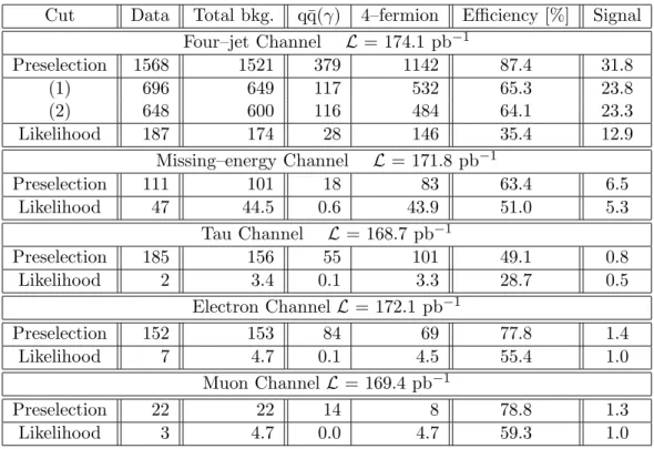
Channel h ⁰ Z ⁰ → Luminosity [pb ⁻¹ ] Data Total bkg. Efficiency [%]

√ s = 183 GeV

b¯ bq¯ q 54.1 7 4.9 ± 0.2 ± 0.6 39.2 ± 0.72 ± 1.2

b¯ bν ν ¯ 53.9 0 1.56 ± 0.13 ± 0.18 47.9 ± 0.4 ± 0.2

b¯ bτ ⁺ τ ⁻ 41.7 ± 2.5 ± 1.8

τ ⁺ τ ⁻ q¯ q 53.7 1 1.3 ± 0.1 ± 0.2

34.2 ± 2.1 ± 1.4 b¯ be ⁺ e ⁻ 53.7 0 0.37 ± 0.07 ± 0.2 68.9 ± 0.8 ± 0.9 b¯ bµ ⁺ µ ⁻ 53.7 1 0.3 ± 0.06 ± 0.1 74.6 ± 0.7 ± 0.7

√ s = 189 GeV

b¯ bq¯ q 172.1 24 19.9 ± 0.8 ± 2.9 47.0 ± 0.8 ± 1.6 b¯ bν ν ¯ 171.4 10 6.9 ± 0.5 ± 0.6 42.6 ± 1.1 ± 1.1

b¯ bτ ⁺ τ ⁻ 44.6 ± 1.8 ± 2.0

τ ⁺ τ ⁻ q¯ q 168.7 3 4.0 ± 0.5 ± 0.9

32.8 ± 1.5 ± 2.1 b¯ be ⁺ e ⁻ 172.1 3 2.6 ± 0.2 ± 0.5 66.3 ± 1.1 ± 1.3 b¯ bµ ⁺ µ ⁻ 169.4 1 2.1 ± 0.1 ± 0.4 78.3 ± 1.1 ± 1.1 Table 1: The h ⁰ Z ⁰ channels: the number of events for the data, the total expected back- ground normalised to the integrated luminosity of the data, and the detection efficiency for a Higgs boson decaying only into b¯ b or τ ⁺ τ ⁻ , for typical masses close to the kine- matical limits of 85 and 95 GeV at √

s = 183 and 189 GeV, respectively. Two separate efficiencies are shown in the tau channel for the two processes h ⁰ → b¯ b, Z ⁰ → τ ⁺ τ ⁻ and h ⁰ → τ ⁺ τ ⁻ , Z ⁰ → q¯q. The first error is statistical and the second systematic.

Higgs boson decays. Detailed descriptions of the flavour independent analyses are given in Sections 4 and 5 for the processes e ⁺ e ⁻ → h ⁰ Z ⁰ and e ⁺ e ⁻ → h ⁰ A ⁰ , respectively.

The channels studied in [29] and [30] using b-tagging, together with those looking for τ –leptons, provide useful information in regions of the 2HDM(II) parameter space where the Higgs bosons are expected to decay predominantly into b¯ b and τ ⁺ τ ⁻ pairs. At

√ s = 183 and 189 GeV, for the process e ⁺ e ⁻ → h ⁰ Z ⁰ the following final states are consid- ered: h ⁰ Z ⁰ → b¯ bq¯q, b¯ bν ν, b¯ ¯ bτ ⁺ τ ⁻ , τ ⁺ τ ⁻ q¯q, b¯ be ⁺ e ⁻ and b¯ bµ ⁺ µ ⁻ . The 2HDM(II) process h ⁰ Z ⁰ → A ⁰ A ⁰ Z ⁰ , followed by A ⁰ → b¯ b, is included when kinematically allowed. In addi- tion, the 2HDM(II) associated production process, e ⁺ e ⁻ → A ⁰ h ⁰ , followed by A ⁰ h ⁰ → b¯ bb¯ b, A ⁰ h ⁰ → b¯ bτ ⁺ τ ⁻ (or τ ⁺ τ ⁻ b¯ b) and h ⁰ A ⁰ → A ⁰ A ⁰ A ⁰ → b¯ bb¯ bb¯ b, is studied.

At √

s ≈ m Z the following final states are interpreted in the framework of the 2HDM(II):

h ⁰ Z ⁰ → q¯qν ν, q¯qτ ¯ ⁺ τ ⁻ , τ ⁺ τ ⁻ q¯q, q¯qe ⁺ e ⁻ and q¯qµ ⁺ µ ⁻ , as well as A ⁰ h ⁰ → q¯qτ ⁺ τ ⁻ (or τ ⁺ τ ⁻ q¯q), and h ⁰ A ⁰ → A ⁰ A ⁰ A ⁰ → b¯ bb¯ bb¯ b, if h ⁰ → A ⁰ A ⁰ is kinematically allowed.

The luminosity, the number of candidate events, the expected SM backgrounds, and

the efficiencies for each of these h ⁰ Z ⁰ and h ⁰ A ⁰ channels at 183 and 189 GeV centre-of-

mass energy are given in Tables 1 and 2, respectively. The signal detection efficiencies

for the process h ⁰ Z ⁰ → A ⁰ A ⁰ Z ⁰ can be found in [29, 30]. The detection efficiencies quoted

in Tables 1 and 2 are given as an example for specific values of m h and m A . When

scanning the parameter space the efficiency is calculated for each point in the (m h , m A )

plane for each of the final states considered. In the tau channel two different final state

topologies are studied, in which h ⁰ → b¯ b, Z ⁰ → τ ⁺ τ ⁻ and h ⁰ → τ ⁺ τ ⁻ , Z ⁰ → q¯q, providing

different efficiencies, as shown in Table 1. The dominant contributions to the systematic

errors on the signal and background efficiencies come from the uncertainty related to

b–tagging [29, 30].

Channel A ⁰ h ⁰ → Luminosity [pb ⁻¹ ] Data Total bkg. Efficiency [%]

√ s = 183 GeV

b¯ bb¯ b 54.1 4 2.92 ± 0.2 ± 0.5 50.3 ± 0.7 ± 2.0 b¯ bτ ⁺ τ ⁻ 53.7 3 1.50 ± 0.1 ± 0.2 44.7 ± 1.6 ± 1.8 b¯ bb¯ bb¯ b 54.1 2 2.3 ± 0.2 ± 0.03 36.0 ± 2.16 ± 1.8

√ s = 189 GeV

b¯ bb¯ b 172.1 8 8.0 ± 0.5 ± 1.4 48.4 ± 0.7 ± 3.9 b¯ bτ ⁺ τ ⁻ 168.7 7 4.9 ± 0.6 ± 1.6 45.3 ± 1.5 ± 2.3 b¯ bb¯ bb¯ b 172.1 5 8.7 ± 1.0 ± 2.5 45.4 ± 2.2 ± 4.3 Table 2: The h ⁰ A ⁰ channels: the number of events for the data, the total expected background normalised to the integrated luminosity of the data and the signal effi- ciency for (m h , m A )=(70 GeV, 70 GeV) and (80 GeV, 80 GeV) in the h ⁰ A ⁰ → b¯ bb¯ b and b¯ bτ ⁺ τ ⁻ channels and for (m h , m A )=(60 GeV, 30 GeV) and (70 GeV, 20 GeV) in the h ⁰ A ⁰ → A ⁰ A ⁰ A ⁰ → b¯ bb¯ bb¯ b channel at √ s= 183 and 189 GeV, respectively. The first error is statistical and the second systematic.

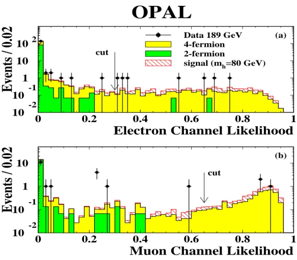
4 Flavour independent searches for e ⁺ e ⁻ → h ⁰ Z ⁰

This section describes the searches for the e ⁺ e ⁻ → h ⁰ Z ⁰ process at √

s= 189 GeV in the following final states: h ⁰ Z ⁰ → q¯qq¯q and ggq¯q (the four–jet channel), h ⁰ Z ⁰ → q¯qν ν ¯ and ggν ν ¯ (the missing–energy channel), h ⁰ Z ⁰ → q¯qτ ⁺ τ ⁻ and ggτ ⁺ τ ⁻ (the tau channel), h ⁰ Z ⁰ → q¯qe ⁺ e ⁻ and gge ⁺ e ⁻ as well as h ⁰ Z ⁰ → q¯qµ ⁺ µ ⁻ and ggµ ⁺ µ ⁻ (the electron and muon channels). A new flavour independent selection has been developed for the four–jet chan- nel. The other channels follow closely the analyses described in reference [30] but do not make use of b–tagging information.

4.1 The four–jet channel

The search in the four–jet channel is a test mass dependent analysis using a binned max-

imum likelihood method. In order to obtain high sensitivity over a wide range of Higgs

boson masses, several likelihood analyses are performed. Each of these is dedicated to

test a specific Higgs mass hypothesis. The test masses are chosen from m h = 60 GeV up

to m h = 100 GeV in steps of 1 GeV, significantly less than the expected mass resolution

for the Higgs boson, which is 2 to 3 GeV. Signal Monte Carlo events have been generated

and reconstructed for each of these test masses. Each likelihood is defined by reference

histograms made from the background Monte Carlo samples and the signal Monte Carlo

events generated at the corresponding mass. All data events are then subjected to each of

the 41 resulting likelihood analyses, and those passing the selection are counted as candi-

dates for masses in a window of ± 0.5 GeV centered on the respective test mass. A single

event can be a candidate at a variety of different test mass values, and the candidates

found in the data are not identical for all mass hypotheses between 60 and 100 GeV.

Correct assignment of particles to jets plays an essential role in separating one of the main backgrounds, W ⁺ W ⁻ → q¯qq¯q, from the signal process, as well as in accurately reconstructing the mass of Higgs bosons in signal events. The jet reconstruction method is explained in [30]. The initial preselection, designed to retain only events with four distinct jets, is unchanged with respect to the four–jet channel in [30] and is independent of any mass hypothesis.

The following selection criteria and the likelihood make explicit use of the mass hy- pothesis:

(1) A kinematic fit which is applied to test the e ⁺ e ⁻ → h ⁰ Z ⁰ hypothesis imposes energy and momentum conservation. Additionally one of the dijet masses is constrained to m Z within its natural width and the other dijet mass is constrained to the tested mass of the Higgs boson (ZH–Fit). This fit is applied to all six possible jet associ- ations and for at least one of these combinations it is required to converge with a χ ² –probability larger than 10 ⁻⁵ . The candidate mass is later calculated using the jet association which yields the highest χ ² –probability.

(2) To discriminate against W ⁺ W ⁻ background, the ratio of the matrix element prob- ability for Higgs–strahlung [31] and the matrix element probability for W ⁺ W ⁻ pro- duction as implemented in EXCALIBUR [18] is required to be larger than 1.2 × 10 ⁻⁴ . When calculating the matrix element probability for Higgs–strahlung it is necessary to assign the measured jets to the original partons. Which jets belong to the decay products of the Z ⁰ and which to the Higgs is determined by the best χ ² –probability of the kinematic fit described in criterion (1). As it remains unknown whether the Z ⁰ decays into up–type or down–type quarks and which jet belongs to the quark and which to the anti–quark, the matrix element is averaged over all these combinations.

Also, the matrix element probability for W ⁺ W ⁻ production is averaged over all pos- sible jet-parton assignments. For both matrix element probabilities the four–vectors after a four–constraint (4C) fit, imposing energy and momentum conservation, are used as input.

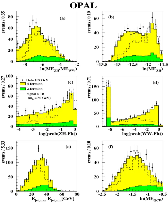
The following six variables are combined with a binned likelihood method [32], with one class for the signal and two for the 4-fermion and the 2-fermion backgrounds:

(a) The logarithm of the ratio of the matrix elements for Higgs–strahlung (ME ZH ) and for W ⁺ W ⁻ production (ME WW ).

(b) The logarithm of the matrix element probability for the Higgs–strahlung process.

In contrast to the kinematic fits, the matrix element also contains angular informa- tion, which allows one to distinguish kinematically between e ⁺ e ⁻ → h ⁰ Z ⁰ and Z ⁰ Z ^{0( ∗)} production, if m h is in the region of m Z . While variable (a) mainly discriminates against W ⁺ W ⁻ events, variable (b) helps to select events compatible with a signal hypothesis. The correlations between (a) and (b) are small.

(c) The logarithm of the χ ² –probability of the ZH–Fit to the Higgs–strahlung hypoth- esis of selection criterion (1). Only the jet association that gives the highest fit probability is considered.

(d) The logarithm of the χ ² –probability resulting from a kinematic fit (WW–Fit), which

in addition to energy and momentum conservation forces both dijet masses to be

OPAL

ln(ME _ZH /ME _WW )

events / 0.35

(a)

ln(ME _ZH )

events / 0.10

(b)

log(prob(ZH-Fit))

events / 0.27

Data 189 GeV (c)

4-fermion 2-fermion signal × 10 (m

= 80 GeV)

log(prob(WW-Fit))

events / 0.71

(d)

E _jet,max -E _jet,min [GeV]

events / 5.33

(e)

ln(ME _QCD )

events / 0.10

(f) 0

20 40 60 80

-8 -6 -4 -2 0

20 40 60

-13.5 -13 -12.5 -12 -11.5

0 20 40 60 80 100

-4 -3 -2 -1 0 0

50 100 150

-8 -6 -4 -2 0

0 50 100 150

0 20 40 60 80 0

20 40 60

-2.5 -2 -1.5 -1 -0.5

Figure 1: Input variables of the four–jet channel likelihood selection for m h = 80 GeV.

The OPAL data are indicated by dots with error bars (statistical errors), the 4-fermion background by lighter grey histograms, and the 2-fermion background by darker grey histograms. All MC distributions are normalised to the integrated luminosity of the data.

The estimated contribution from an 80 GeV SM Higgs boson, scaled up by a factor of 10,

is shown with a dashed line in each case.

0 20 40 60 80 100 120 140

0 0.2 0.4 0.6 0.8 1

OPAL

likelihood

events / 0.05 cut

(a) Data 189 GeV

signal (m _h =75 GeV) 4-fermion

2-fermion

likelihood

events / 0.05

cut

(b) Data 189 GeV

signal (m _h =95 GeV) 4-fermion

2-fermion

0 20 40 60 80 100 120 140

0 0.2 0.4 0.6 0.8 1

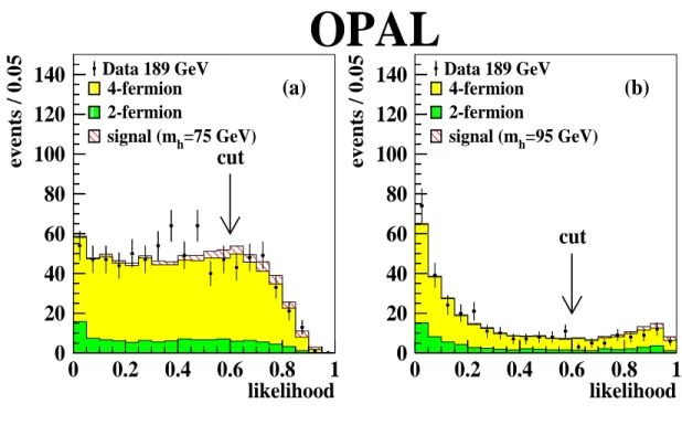
Figure 2: Likelihood distribution of the four–jet channel for test masses of (a) 75 GeV and (b) 95 GeV. The OPAL data are indicated by dots with error bars (statistical errors), the 4-fermion background by lighter grey histograms, and the 2-fermion background by darker grey histograms. The contributions expected from a (a) 75 GeV and (b) 95 GeV h ⁰ boson assuming SM cross–section and branching ratios are shown as hatched histograms.

All MC distributions are normalised to the integrated luminosity of the data. All events with a likelihood larger than 0.6 are accepted.

equal to the mass of the W boson. Only the jet association that gives the highest fit probability is considered.

(e) The difference between the largest and the smallest jet energies in the event.

(f) The logarithm of an event weight, ME QCD , formed [33] from the tree level matrix element for the process e ⁺ e ⁻ → q¯qq¯q, q¯qgg [34], to reduce QCD background.

In Figure 1 the distributions of the likelihood input variables are shown for the difficult case in which m h ≈ m W .

The distributions of the final likelihood L ^hZ are shown in Figure 2 for test masses of

75 and 95 GeV. Candidates for signal production are required to have L ^hZ > 0.6 for

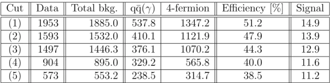
all test masses. In Table 3 the numbers of observed and expected events, together with

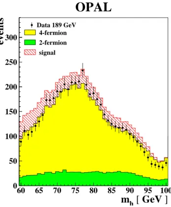
the detection efficiencies for a Higgs signal with a mass of 80 GeV, are given. Figure 3

compares the number of candidate events obtained after the likelihood selections for the

different test masses with the expected background evaluated from Monte Carlo simula-

tions. In the region of 75 GeV, the number of expected background events rises to more

than 200. This is due to the presence of W ⁺ W ⁻ events, where the mass of one of the W

bosons is constrained to the mass of the Z ⁰ , which reduces the other dijet mass by a few

0 50 100 150 200 250 300

60 65 70 75 80 85 90 95 100

OPAL

m _h [ GeV ]

events

Data 189 GeV

signal 4-fermion 2-fermion

Figure 3: Number of events that pass the four–jet channel selection at each test mass.

The number of candidates found in the data is indicated by dots with error bars (sta- tistical errors), and the darker and lighter grey histograms correspond to the number of events expected from 2-fermion and 4-fermion backgrounds, respectively. The expected contribution from a Higgs boson with a mass equal to the test mass, assuming SM cross–

sections and branching ratios, is shown by the hatched histogram. All MC distributions are normalised to the integrated luminosity of the data. Each bin corresponds to a dif- ferent analysis of the same data, leading to a strong correlation between neighbouring bins.

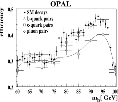
GeV compared to the nominal value. The candidate masses are calculated from the momenta resulting from a 5C fit requiring energy and momentum conservation and forcing one of the dijet masses to m Z . Figure 4 shows the efficiency as a function of the Higgs mass for decays to b–quark, c-quark and gluon pairs separately as well as for a mixed sample according to SM branching ratios. For m h between 80 and 95 GeV the efficiency reaches about 40 to 45% for quarks and 35% for gluons. For small values of m h it drops to 25% due to the relatively large amount of initial state radiation that accompanies Higgs–strahlung when m h is considerably lower than the kinematic limit, i.e. √

s − m Z . For the limit calculation, the efficiencies have been fitted to a polynomial function of m h

for each flavour separately, and at each mass point the lowest fitted polynomial is used.

The signal selection efficiencies are affected by the uncertainties given below, expressed in

relative percentages and shown as an example for a Higgs mass of 75 GeV. The systematic

errors have been evaluated as follows: for each variable, the distributions obtained from

the background Monte Carlo samples have been compared to those in the data. Then all

Monte Carlo events (including the signal samples) have been reweighted so that the mean

values of data and background distributions become the same and so that the sum of all

0.2 0.3 0.4 0.5

60 65 70 75 80 85 90 95 100

SM decays b-quark pairs c-quark pairs gluon pairs

m h [ GeV ]

efficiency

OPAL

h [ GeV]

m

Figure 4: Efficiency of the four–jet channel selection as a function of m h determined from different Monte Carlo samples. The dots represent the efficiency obtained from samples with SM branching ratios which also define the reference histograms at each test mass.

The triangles, squares and crosses correspond to independent samples where the Higgs boson decays exclusively to b–quark, c–quark or gluon pairs, respectively. For the limit calculation, efficiencies have been fitted to a polynomial function of m h for each flavour separately, and at each mass point the lowest fitted polynomial is used (black line).

weights is equal to 1. The relative deviations in the number of events which pass the selection obtained by reweighting according to the different variables have been added in quadrature and amount to 5.5%. The same procedure has been applied to the kine- matic likelihood variables, yielding an uncertainty of 2.0%. The uncertainty on the error parameterisation of the jet momenta used in the kinematic fits has been evaluated by varying the energy and angular resolutions by ± 10% , the energy scale by ± 1% and the centre–of–mass energy by ± 0.3 GeV, each time repeating all kinematic fits. This leads to an uncertainty of 6.4%. Since the steps in the test mass are chosen to be smaller than the expected mass resolution, the deviation in efficiency due to the interpolation between test masses amounts only to 0.7%. The total systematic uncertainty on the signal selection efficiency has been calculated by adding the above sources in quadrature yielding 8.7%.

All of these error contributions have been evaluated for masses of 60 and 90 GeV as well, leading to total systematic uncertainties of 9.8% and 7.1%, respectively. The Monte Carlo statistical error is about 2%.

The following uncertainties on the two major background sources are taken into ac-

count (the first number corresponds to the 4-fermion, the second number to the q¯q(γ)

background, both for a test mass of 75 GeV): the uncertainty from modelling of the

preselection cuts is evaluated as described above and amounts to 5.2%/4.5%. For the

likelihood variables this procedure leads to an uncertainty of 1.2%/1.6%. Varying the

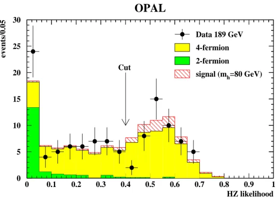
OPAL

HZ likelihood

events/0.05

Cut

Data 189 GeV 4-fermion 2-fermion

signal (m _h =80 GeV)

0 5 10 15 20 25 30

0 0.1 0.2 0.3 0.4 0.5 0.6 0.7 0.8 0.9 1

Figure 5: Likelihood output of the missing energy channel selection. The OPAL data are indicated by dots with error bars (statistical errors), the 4-fermion background by the lighter grey histogram, and the 2-fermion background by the darker grey histogram. The estimated contribution from an 80 GeV Higgs with SM cross–section and branching ratios is shown as a hatched histogram. All MC distributions are normalised to the integrated luminosity of the data.

error parameterisations, energy scale and centre–of–mass energy for the kinematic fits yields an uncertainty of 3.0%/8.1%. Different Monte Carlo generators have been used to evaluate the background from 4-fermion events (EXCALIBUR instead of grc4f) and QCD events (HERWIG instead of PYTHIA) resulting in an uncertainty of 2.2%/12.3%. The total systematic uncertainty on the residual background estimate amounts to 10.3%. For test masses of 60 and 90 GeV the total systematic uncertainties amount to 12.4% and 8.3%, respectively. The largest Monte Carlo statistical error is 1.3%.

4.2 The missing–energy channel

This analysis is nearly identical to a previous one, of which a detailed description can

be found in [29], with the exception that the b–tagging is not applied. The preselection

is unchanged. The same kinematic variables used previously, as well as the acollinearity

angle and the total missing transverse momentum, are combined using a likelihood tech-

nique. In Figure 5, the resulting signal likelihood distribution is shown for the data, SM

backgrounds, and an example signal at m h = 80 GeV. The signal likelihood is required

to be larger than 0.4 for an event to be selected as a Higgs candidate.

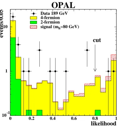
OPAL

10 ^-1 1 10

0 0.2 0.4 0.6 0.8 1

likelihood

events/0.05

cut

Data 189 GeV 4-fermion 2-fermion

signal (m _h =80 GeV)

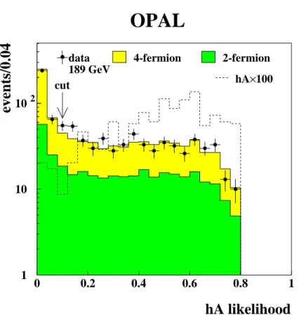
Figure 6: Likelihood output of the tau channel selection for events satisfying the h ⁰ Z ⁰ → q¯qτ ⁺ τ ⁻ kinematic hypothesis. OPAL data are indicated by dots with error bars (statistical errors), 4-fermion background by the lighter grey histogram, and 2-fermion background by the darker grey histogram. The contribution expected from an 80 GeV Higgs with SM cross–section and branching ratios is shown as a hatched histogram. All MC distributions are normalised to the integrated luminosity of the data.

The reconstructed mass in selected events is evaluated using a kinematic fit constrain- ing the recoil mass to the Z ⁰ mass. The numbers of observed and expected events ³ are given in Table 3, together with the selection efficiencies for an 80 GeV Higgs. The se- lection efficiency has been estimated from Monte Carlo samples generated separately for b–quark, c–quark and gluon pairs. The efficiency is the lowest and the width of the re- constructed Higgs mass is the largest for c–quark pairs and therefore they are used in the limit calculation. For an 80 GeV Higgs, the efficiency is (51.0 ± 1.7(stat.) ± 1.3(syst.))%.

The efficiency has been optimised for Higgs masses between 70 and 90 GeV. Outside this range, the efficiency decreases and reaches about 20% for masses of 60 and 100 GeV. For b–quarks, the efficiency is about 5% (relative) higher throughout the whole mass range.

A total of 47 data events pass the selection, while 44.5 ± 1.4(stat.) ± 3.0(syst.) events are expected from SM background processes. The systematic error has been evaluated as in [29], but b–tagging related errors have been omitted.

3

In the calculation of the efficiencies and backgrounds in the missing–energy channel, a 2.5% relative

reduction has been applied to the Monte Carlo estimates in order to account for accidental vetoes due to

accelerator related backgrounds in the forward detectors.

4.3 The tau channel

The preselection, the tau lepton identification using an artificial neural network, and the two–tau likelihood, L ^{τ τ} , used in this channel are unchanged with respect to the analysis described in reference [30]. Since b–tagging information is not used, for the final selection the likelihood L (q¯qτ ⁺ τ ⁻ ) [30] is used and required to exceed 0.8. Additionally, the χ ² – probability of a kinematic fit, which constrains the invariant mass of the two τ’s to m Z , should be larger than 10 ⁻⁵ , since this analysis is designed to be sensitive to hadronic Higgs boson decays and to Z ⁰ → τ ⁺ τ ⁻ . In Figure 6 the resulting likelihood distributions are shown for the data, SM backgrounds, and an example signal at m h = 80 GeV. The numbers of observed and expected events are given in Table 3, together with the selection efficiencies for an 80 GeV Higgs. The signal detection efficiency has been evaluated for b–quark, c–

quark and gluon pairs separately and at each mass the lowest value is taken for the limit calculation. For an 80 GeV Higgs boson it amounts to (28.7 ± 1.5(stat.) ± 2.7(syst.))%

after all the selection requirements. For lower and higher Higgs masses, the efficiency drops to about 20% at m h = 50 GeV and m h = 100 GeV. Two events survive the likelihood cut, which can be compared to the expected background of 3.4 ± 0.5(stat.) ± 0.7(syst.). The systematic errors quoted above for signal and background are evaluated with the method described in [29], with the contributions from fragmentation and decay multiplicity of b–quarks omitted.

4.4 The electron and muon channels

The preselection cuts and kinematic likelihood K are identical to the analysis described in [29]. Because the present analysis is intended to be independent of the flavour of the Higgs decay products, no b–tagging is applied and K is used as the final selection variable, which should exceed 0.3 for the electron and 0.65 for the muon channel. Figure 7 shows the distribution of K for the electron (a) and the muon (b) channel.

The signal selection efficiency has been evaluated and fitted for each flavour separately.

For the limit calculation, the lowest of these efficiencies at each mass point has been used.

For an 80 GeV Higgs boson it amounts to (55.4 ± 1.6(stat.) ± 0.6(syst.))% for the electron channel, and (59.3 ± 1.5(stat.) ± 0.7(syst.))% for the muon channel. In the electron channel, the efficiency lies between 50% and 55% for all Higgs masses between 60 and 95 GeV, and drops to 27% for a Higgs mass of 100 GeV. In the muon channel, the efficiency is between 55% and 70% for all Higgs masses under consideration.

The numbers of observed and expected events are given in Table 3, together with the detection efficiency for an 80 GeV SM Higgs boson. The selection retains 7 events in the electron channel and 3 in the muon channel. The total background expectation is 4.7 ± 0.2(stat.) ± 1.4(syst.) events in the electron channel and 4.7 ± 0.1(stat.) ± 0.9(syst.) events in the muon channel.

The systematic errors quoted above for signal and background are evaluated with

the method described in [29]. The largest contribution to the systematic error on the

background expectation is due to differences between various Monte Carlo generators.

OPAL

Electron Channel Likelihood

Events / 0.02

(a) cut

Data 189 GeV 4-fermion 2-fermion

signal (m _h =80 GeV)

Muon Channel Likelihood

Events / 0.02

(b) cut

10 ^-2 10 ^-1

1 10 10 ²

0 0.2 0.4 0.6 0.8 1

10 ^-2 10 ^-1

1 10

0 0.2 0.4 0.6 0.8 1

Figure 7: (a) The electron and (b) the muon channel likelihood distributions. The OPAL data are indicated by dots with error bars (statistical), the 4-fermion background by lighter grey histograms, and the 2-fermion background by darker grey histograms. The contributions expected from an 80 GeV Higgs with SM cross–section and branching ratios are shown as hatched histograms. All MC distributions are normalised to the integrated luminosity of the data.

4.5 Summary of the flavour independent searches for e ⁺ e ⁻ → h ⁰ Z ⁰

The total numbers of candidates accepted after the preselection and the flavour indepen-

dent likelihood cut, compared to the expected SM backgrounds as well as the detection

efficiencies for a hadronically decaying Higgs boson with a mass of 80 GeV, are sum-

marised in Table 3, together with the expected number of signal events in the 2HDM(II)

for the case of α = 0, tanβ = 1.0 and m h = 80 GeV. The total number of observed

candidates for an 80 GeV Higgs boson is 246, while the background expectation amounts

to 231.3 ± 4.4(stat.) ± 18.0(syst.).

Cut Data Total bkg. q¯ q(γ) 4–fermion Efficiency [%] Signal Four–jet Channel L = 174.1 pb ⁻¹

Preselection 1568 1521 379 1142 87.4 31.8

(1) 696 649 117 532 65.3 23.8

(2) 648 600 116 484 64.1 23.3

Likelihood 187 174 28 146 35.4 12.9

Missing–energy Channel L = 171.8 pb ⁻¹

Preselection 111 101 18 83 63.4 6.5

Likelihood 47 44.5 0.6 43.9 51.0 5.3

Tau Channel L = 168.7 pb ⁻¹

Preselection 185 156 55 101 49.1 0.8

Likelihood 2 3.4 0.1 3.3 28.7 0.5

Electron Channel L = 172.1 pb ⁻¹

Preselection 152 153 84 69 77.8 1.4

Likelihood 7 4.7 0.1 4.5 55.4 1.0

Muon Channel L = 169.4 pb ⁻¹

Preselection 22 22 14 8 78.8 1.3

Likelihood 3 4.7 0.0 4.7 59.3 1.0

Table 3: The h ⁰ Z ⁰ channels for the flavour independent analysis: the numbers of events selected in the data at √

s = 189 GeV, expected background from SM processes normalised to the data luminosity (given for each channel), the minimal detection efficiencies for a Higgs boson with a mass of 80 GeV decaying to quark or gluon pairs and the expected number of signal events within the 2HDM(II) for the case of α = 0, tanβ = 1.0 and m h = 80 GeV, after the preselection and the flavour independent likelihood cut. In the case of the four–jet channel, after preselection, the numbers of events are given for the selection with an 80 GeV test mass.

0 5 10 15 20 25 30 35 40

55 60 65 70 75 80 85 90 95 100

m _h [GeV]

events / 1.5 GeV

Data 189 GeV

4-jet channel

missing-energy channel tau channel

muon channel electron channel

( a )

OPAL

0 2 4 6 8 10 12 14

55 60 65 70 75 80 85 90 95 100

m _h [GeV]

events / 3 GeV

Data 189 GeV

missing-energy channel tau channel

muon channel electron channel

( b )

Figure 8: Mass distributions for selected data events and SM background expectation

(a) for all channels and (b) for all channels except the four–jet channel. OPAL data are

indicated by dots with error bars (statistical) while the background contributions from

the various channels are shown in different shades of grey. For the four–jet channel the

90 GeV analysis is shown.

The mass distributions for candidates found in the data as well as for the background expected from the SM for all flavour independent channels are shown in Figure 8(a). The same mass distributions without the four–jet channel contribution are shown in Figure 8(b).

5 Flavour independent search for e ⁺ e ⁻ → h ⁰ A ⁰

We have searched for the process e ⁺ e ⁻ → h ⁰ A ⁰ in the final states q¯qq¯q, ggq¯q and gggg. The signal is characterised by events with four well-separated jets with characteristic invariant masses of the dijet pairs originating from the h ⁰ and the A ⁰ . The dominant background is from the process e ⁺ e ⁻ → W ⁺ W ⁻ → q¯qq¯q. The second-largest contribution comes from e ⁺ e ⁻ → Z ⁰ /γ → q¯q with multiple hard gluon radiation producing a four–jet final state.

This search is designed to be sensitive over a large portion of the (m h , m A ) plane, and the kinematic signatures of signal events depend strongly on m h and m A . For this reason, a loose selection is performed first, retaining four-jet hadronic events with partial rejection of W ⁺ W ⁻ and Z ⁰ Z ⁰ events. The main discrimination, however, is achieved by constraining candidate events to the signal mass hypothesis (m h and m A ), and using the logarithm of the resulting χ ² as the discriminant variable in the limit calculation instead of the reconstructed dijet masses. This choice of variable also incorporates naturally the measurement uncertainties on the reconstructed masses and simplifies the interpolation of its shape as a function of m h and m A .

5.1 Selection

Candidate events must first satisfy the requirements of a preselection and then a loose selection based on a likelihood variable which is built out of reference distributions of reconstructed quantities for events passing the preselection. The following criteria are applied ((1)–(4) preselection, (5) selection):

(1) Each candidate event is required to be classified as a hadronic final state [35] with an effective centre-of-mass energy √

s ^′ exceeding 150 GeV. The jet resolution parameter in the Durham scheme [13] y 34 is required to be larger than 0.003 in order to select events with four distinct jets.

(2) Each jet must have at least three tracks.

(3) The χ ² probability of a 4C fit, requiring energy and momentum conservation, must be greater than 10 ⁻⁵ , to ensure that the mass reconstructions used to isolate the signal do not suffer from poor measurement or energy loss from initial state radia- tion.

(4) A 6C kinematic fit is performed requiring energy and momentum conservation and

also that the invariant masses of the dijet pairs are equal to m W . The 6C fit χ ²

probability of each of the three possible jet combinations is required to be less than

0.01, to reduce the background from hadronic W ⁺ W ⁻ decays.

Cut Data Total bkg. q¯q(γ) 4-fermion Efficiency [%] Signal

(1) 1953 1885.0 537.8 1347.2 51.2 14.9

(2) 1593 1532.0 410.1 1121.9 47.9 13.9

(3) 1497 1446.3 376.1 1070.2 44.3 12.9

(4) 904 895.0 329.2 565.8 40.0 11.6

(5) 573 553.2 238.5 314.7 38.5 11.2

Table 4: The h ⁰ A ⁰ channel for the flavour independent analysis: the numbers of events selected in the data at √

s = 189 GeV, expected background from SM processes normalised to the data luminosity of 172.1 pb ⁻¹ , the minimal detection efficiencies for m h = 30 GeV, m A = 60 GeV and the expected number of signal events within the 2HDM(II) for the case of α = 0, tanβ = 1.0, m h = 30 GeV and m A = 60 GeV after each step of the selection.

(5) A likelihood composed of five variables is computed. These variables are the jet resolution parameter y 34 , the event-shape variable C obtained from the eigenvalues of the sphericity tensor [36], the smallest angle between any two jets in the event, the logarithm of the QCD matrix element ME QCD [34], and the largest χ ² proba- bility of three 5C kinematic fits constraining energy and momentum and requiring the equality of the masses of the two dijet systems (three possible pairings). The QCD matrix element used is the maximum of the matrix elements considering all possible assignments of observed jets to partons in the e ⁺ e ⁻ → q¯qq¯q and e ⁺ e ⁻ → q¯qgg processes. The first four variables are designed to separate the signal from the q¯q background. The last variable provides rejection of the diboson backgrounds from W ⁺ W ⁻ and Z ⁰ Z ⁰ events surviving the 6C fit probability requirement (4). Although its use reduces the efficiency for signals with m _h = m _A , the sensitivity to signals with m h 6 = m A is enhanced. The signal samples used to form reference distributions for the likelihood are a mixture of samples in the kinematically accessible region of the (m _h , m _A ) plane with m _h , m _A > 30 GeV. The distribution of this likelihood variable for the data, SM backgrounds, and a representative signal with m h = 30 GeV and m A = 60 GeV is shown in Figure 9. The likelihood variable is required to exceed 0.1 for selected events.

In Table 4 the numbers of events passing the requirements after each step, (1) to (5), are given, together with the expected SM backgrounds from 4-fermion and 2-fermion processes. The lowest estimated efficiencies, for m h = 30 GeV and m A = 60 GeV, cor- responding to the b¯ bb¯ b final state, and the number of expected signal events in the 2HDM(II) for the case of α = 0, tanβ = 1.0, m h = 30 GeV and m A = 60 GeV, are shown in the last two columns.

The selection efficiency is estimated with the Monte Carlo simulation at a discrete set of reference points in the (m h , m A ) plane. The efficiency function is interpolated by considering the three closest reference points. A plane in the (m _h , m _A , efficiency) space is formed containing those three points, which allows the efficiency for an arbitrary inter- mediate (m h , m A ) signal hypothesis to be computed. The interpolated efficiency function is shown in Figure 10 for the final-state flavour assignment with the lowest efficiency.

The efficiency is low near m h = m A = m W because of the difficulty in distinguishing

hadronic h ⁰ A ⁰ decays from hadronic W ⁺ W ⁻ decays. The veto of W ⁺ W ⁻ events reduces

1 10 10 ²

0 0.2 0.4 0.6 0.8 1

OPAL

hA likelihood

events/0.04

hA × 100 data

189 GeV

4-fermion 2-fermion cut

Figure 9: Likelihood distribution for the flavour independent e ⁺ e ⁻ → h ⁰ A ⁰ channel. The OPAL data are indicated by dots with error bars (statistical error), the 4-fermion back- ground by the lighter grey histogram, the 2-fermion background by the darker grey his- togram and a representative signal for m h = 30 GeV, m A = 60 GeV by the dashed histogram. All Monte Carlo distributions are normalised to the data luminosity and the signal is scaled by a factor of 100.

the efficiency in the entire (m h , m A ) plane because incorrect jet assignments in h ⁰ A ⁰ events can produce interpretations consistent with the W ⁺ W ⁻ hypothesis. Conversely, the W ⁺ W ⁻ veto reduces the background of incorrectly-paired W ⁺ W ⁻ events everywhere in the (m h , m A ) plane. The efficiency for low m h and m A is reduced because of the requirement that the event should have four distinct jets, which helps to reject the q¯q background.

After the selection, 573 candidates remain in the data, as compared with the SM expectation of 553.2 ± 38.2 events.

5.2 Discriminant variable

The invariant masses of jet pairs may be used to separate possible h ⁰ A ⁰ signals from the

W ⁺ W ⁻ and q¯qgg backgrounds. There are six possible assignments of pairs of jets to h ⁰

and A ⁰ bosons, and there is no constraint from a known mass such as that of the Z ⁰ used

in the e ⁺ e ⁻ → h ⁰ Z ⁰ channels. All six possible interpretations of each selected event are

tested for consistency with a possible signal. When computing the confidence level for

excluding a model hypothesis, only a single interpretation of each candidate in the data

40 60 80 100 120 140 160

40 60 80 100 120 140 160

m _h [GeV]

m A [GeV]

0.1 0.2 0.3 0.3

0.3

0.4 0.5

0.4 0.5 0.4

OPAL

OPAL

Figure 10: Lowest efficiency contours for the flavour independent search for hadronic h ⁰ A ⁰ events. The efficiency is taken to be zero for m h +m A > 189 GeV.

and Monte Carlo samples may be used. The choice of jet pairing depends on the m h and m A of the hypothesised signal.

For each event passing the selection, a 4C kinematic fit constraining energy and mo- mentum conservation is performed. For each of the assignments of jet pairs to bosons, the reconstructed m h and m A are computed, along with their covariance matrices. For each hypothetical m h and m A considered in the limit computation, each event is assigned the jet pairing with the smallest χ ² value resulting from the difference of the measured and hypothesised m h and m A , and the error matrix of the measurement. The logarithm of the smallest χ ² is then used as the discriminating variable when computing limits because the signal to background ratio depends strongly on the value of log χ ² . Figure 11 shows the distribution of log χ ² for selected data events, the SM expectation, and the signal for four mass hypotheses. The signal shown corresponds to the e ⁺ e ⁻ → h ⁰ A ⁰ → gggg process because of its poorer mass resolution compared with that obtained for final states with quarks.

For m h = m A = m W , the separation between the signal and the background is poor,

while for lower values of m _h or m _A the separation is better. The resolution on the

reconstructed sum of the dijet masses is approximately 2.4 GeV, while for the difference

it is approximately 6.2 GeV. The best sensitivity to the signal is in regions of (m h , m A )

with dijet mass sums different from 2m W . The test mass spacing is determined by the

model scan grid used when computing the limits – no discretization is introduced within

the analysis. The scan grid used to compute limits has a finer spacing than the mass

resolutions on the candidates. All candidates are considered at all test mass hypotheses –

they simply appear at different locations in the log χ ² histogram. The distribution of the

χ ² variable for the signal and backgrounds changes slowly with the test mass hypothesis