Finite Combinatory Logic with Intersection Types

Finite Combinatory Logic with Intersection Types

Jakob Rehof

and Pawe l Urzyczyn

1

Technical University of Dortmund Department of Computer Science jakob.rehof@cs.tu-dortmund.de

2

University of Warsaw Institute of Informatics urzy@mimuw.edu.pl

Abstract. Combinatory logic is based on modus ponens and a schematic (polymorphic) interpretation of axioms. In this paper we propose to consider expressive combinatory logics under the restriction that ax- ioms are not interpreted schematically but ,,literally”, corresponding to a monomorphic interpretation of types. We thereby arrive at finite com- binatory logic, which is strictly finitely axiomatisable and based solely on modus ponens. We show that the provability (inhabitation) problem for finite combinatory logic with intersection types is Exptime -complete with or without subtyping. This result contrasts with the general case, where inhabitation is known to be Expspace -complete in rank 2 and undecidable for rank 3 and up. As a by-product of the considerations in the presence of subtyping, we show that standard intersection type subtyping is in Ptime . From an application standpoint, we can consider intersection types as an expressive specification formalism for which our results show that functional composition synthesis can be automated.

1 Introduction

Under the Curry-Howard isomorphism, combinatory terms correspond to Hilbert- style proofs, based on two principles of deduction: modus ponens and a schematic interpretation of axioms. The latter can be expressed as a meta-rule of instan- tiation or as a rule of substitution. The schematic interpretation corresponds to considering types of combinators as implicitly polymorphic.

Because of the schematic interpretation of axioms, such logics are not strictly finite.

In the present paper we propose to consider finite combinatory logics. Such logics arise naturally from combinatory logic by eliminating the schematic in- terpretation of axioms. This corresponds to a monomorphic interpretation of combinator types, and leaves modus ponens as the sole principle of deduction.

We consider combinatory logic with intersection types [4]. In general, the prov- ability problem for this logic is undecidable. We prove that provability in finite

?

Partly supported by MNiSW grant N N206 355836.

3

The schematic viewpoint is sometimes referred to as typical ambiguity.

combinatory logic is decidable and Exptime -complete. We show, in fact, that all of the problems: emptiness, uniqueness and finiteness of inhabitation are in Exp- time by reduction to alternating tree automata. We then consider the provability problem in the presence of standard intersection type subtyping. We show that the subtyping relation is in Ptime (previous work only appears to establish an exponential algorithm). We prove that provability remains Exptime -complete in the presence of subtyping, and also that uniqueness and finiteness of inhab- itation remain in Exptime . In contrast to the case without subtyping, which is solved by reduction to tree automata, the upper bounds are achieved using polynomial space bounded alternating Turing machines.

From an application standpoint, we are interested in finite combinatory logic with intersection types as an expressive specification logic for automatic function composition synthesis. Under the Curry-Howard isomorphism, validity is the question of inhabitation: Given a set Γ of typed combinators (function symbols), does there exist an applicative combination e of combinators in Γ having a given type τ? An algorithm for inhabitation in finite combinatory logic can be used to synthesize e from the specification given by Γ and τ.

Due to space limitations some proofs have been left out. All details can be found in the technical report [16] accompanying this paper.

Finite combinatory logic with intersection types. The strictly finite standpoint considered here is perhaps especially interesting for highly expressive logics for which validity is undecidable. Intersection type systems [3, 15] belong to a class of propositional logics with enormous expressive power. Intersection types cap- ture several semantic properties of lambda terms, and their type reconstruction problem has long been known to be undecidable, since they characterize exactly the set of strongly normalizing terms [15]. Intersection types have also been used more generally to capture semantic properties of programs, for example in the context of model checking [13, 7]. The inhabitation problem for the λ-calculus with intersection types was shown to be undecidable in [18] (see also [17] for connections to λ-definability). More recently, the borderline between decidabil- ity and undecidability was clarified in [10, 19] by rank restrictions (as defined in [11]), with inhabitation in rank 2 types being shown Expspace -complete and undecidable from rank 3 and up.

Combinatory logic with intersections types was studied in [4], where it was shown that the combinatory system is complete in that it is logically equivalent to the λ-calculus by term (proof) translations in both directions. It follows that provability (inhabitation) for combinatory logic with intersections types is undecidable.

Application perspective. Finite combinatory logic can be used as a foundation for automatic composition synthesis via inhabitation: Given a set Γ of typed functions, does there exist a composition of those functions having a given type? Under this interpretation, the set Γ represents a library of functions, and the intersection type system provides a highly expressive specification logic

4

Other restrictions have also been considered, which arise by limiting the logic of

intersection [9, 20].

for which our results show that the problem of typed function composition syn- thesis can be automated. Our approach provides an alternative to synthesis via proof counting (following [2]) for more complex term languages (e.g., [22]).

Most notably, finite combinatory logic is naturally applicable to synthesis from libraries of reusable components which has been studied recently [12], leading to a 2 Exptime -complete synthesis problem. Our setting is different, since our framework is functional (rather than reactive), it is based on a different speci- fication format (types rather than temporal logic), so we obtain an Exptime - complete problem (using the identity Apspace = Exptime ). We gain algorith- mic control over the solution space to the synthesis problem, since it follows from the reduction that not only the problem of inhabitation but also the problems of finiteness and uniqueness of inhabitation are solvable in Exptime . The incorpo- ration of subtyping is important here, since it would allow synthesis specifications to take advantage of hierarchical structure, such as inheritance or taxonomies.

Although synthesis problems are by nature computationally complex, the exploitation of abstraction in component libraries and type structure allows new ways of scaling down problem size. An implementation of the algorithms described here is currently underway in the context of a component synthesis framework, and future work will address experimental evaluation.

2 Preliminaries

Trees: Let A and L be non-empty sets. A labeled tree over the index set A and the alphabet of labels L is understood as a partial function T : A

→ L, such that the domain dm(T ) is non-empty and prefix-closed. The size of T , denoted |T|, is the number of nodes in (the domain of) T . The depth of a tree T, written k T k, is the maximal length of a member of dm(T ). Note that k T k ≤ |T |. For w ∈ dm(T ), we write T [w] for the subtree of T rooted at w, given by T[w](w

) = T (ww

).

Terms: Applicative terms, ranged over by e etc., are defined by:

e ::= x | (e e

),

where x, y, z etc. range over a denumerable set of variables. We write e ≡ e

for syntactic identity of terms. We abbreviate (. . . ((e e

) e

) . . . e

) as (e e

e

. . . e

) for n ≥ 0 (for n = 0 we set (e e

. . . e

) ≡ e). Notice that any applicative term can be written uniquely as (x e

. . . e

).

An alternative to the above standard understanding of expressions as words,

is to represent them as finite labeled trees over the index set N and the alphabet

V ∪ ( N − {0}). A variable x is seen as a one-node tree where the only node is

labeled x. An expression (x e

. . . e

) is a tree, denoted @

(x, e

, . . . , e

), with

root labeled @

and n + 1 subtrees x, e

, . . . , e

, which are addressed from left

to right from the root by the indices 0, 1, . . . , n. That is, if e = @

(x, e

, . . . , e

),

we have e(ε) = @

, e(0) = x and e(i) = e

for i = 1, . . . , n. In a term of the

form @

(x, e

, . . . , e

) we call the tree node x the operator of node @

. We say

that a variable x occurs along an address w ∈ dm(e) if for some prefix u of w we

have u0 ∈ dm(e) with e(u0) = x.

Types: Type expressions, ranged over by τ, σ etc., are defined by τ ::= α | τ → τ | τ ∩ τ

where α ranges over a denumerable set T V of type variables. We let T de- note the set of type expressions. As usual, types are taken modulo idempotency (τ ∩ τ = τ), commutativity (τ ∩ σ = σ ∩ τ), and associativity ((τ ∩ σ) ∩ ρ = τ ∩ (σ ∩ ρ)). A type environment Γ is a finite set of type assumptions of the form x : τ , and we let dm(Γ ) and rn(Γ ) denote the domain and range of Γ .

A type τ ∩ σ is said to have τ and σ as components. For an intersection of several components we sometimes write T

i=1

τ

or T

i∈I

τ

. We stratify types by letting A, B, C, . . . range over types with no top level conjunction, that is

A ::= α | τ → τ We can write any type τ as T

i=1

A

for suitable n ≥ 1 and A

.

Types as trees: It is convenient to consider types as labeled trees. A type tree τ is a labeled tree over the index set A = N ∪ {l, r} and the alphabet of labels L = T V ∪ {→, ∩}, satisfying the following conditions for w ∈ A

:

• if τ(w) ∈ TV , then {a ∈ A | wa ∈ dm(τ)} = ∅;

• if τ(w) = →, then {a ∈ A | wa ∈ dm(τ)} = {l, r};

• if τ(w) = ∩, then {a ∈ A | wa ∈ dm(τ)} = {1, . . . , n}, for some n.

Trees are identified with types in the obvious way. Observe that a type tree is Logspace -computable from the corresponding type and vice versa. Recall that types are taken modulo idempotency, commutativity and associativity, so that a type has in principle several tree representations. In what follows we always assume a certain fixed way in which a type is interpreted. By representing A as T

i=1

A

we can assume w.l.o.g. that types τ are alternating, i.e., that all

w ∈ dm(τ) alternate between members of N and {l, r} beginning and ending

with members of N , and we call such w alternating addresses. We define right-

addresses to be members of A

with no occurrence of l. For an alternating

type τ, we define R

(τ) to be the set of alternating right-addresses in dm(τ)

with n occurrences of r. Observe that alternating right-addresses have the form

n

rn

r . . . rn

with n

∈ N for 0 ≤ j ≤ k, in particular note that R

(τ) =

{1, . . . , k}, for some k. For w ∈ R

, n ≥ 1 and 1 ≤ j ≤ n, we let w ↓ j

denote the address that arises from chopping off w just before the j’th occurrence

of r in w, and we define L(j, w) = (w ↓ j)l. The idea is that alternating right-

addresses in τ determine “target types” of τ, i.e., types that may be assigned to

applications of a variable of type τ. For example, if τ = ∩{α

∩ α

→ β

∩ β

},

then we have 1r1, 1r2 ∈ R

(τ) with τ[1r1] = β

and τ[1r2] = β

. Moreover,

τ[L(1, 1r1)] = τ[1l] = α

∩ α

. Now suppose that x : τ and observe that an

expression (x e) can be assigned any of types β

and β

, provided e : α

∩ α

.

Definition 1 (arg , tgt). The j’th argument of τ at w is arg(τ, w, j) = τ [L(j, w)],

and the target of τ at w is tgt (τ, w) = τ[w].

Definition 2 (Sizes). The size (resp. depth) of a term or type is the size (resp. depth) of the corresponding tree. The size of an environment Γ is the sum of the cardinality of the domain of Γ and the sizes of the types in Γ , i.e.,

|Γ | = |dm(Γ )| + P

x∈dm(Γ)

|Γ (x)|. Also we let k Γ k denote the maximal depth of a member of rn(Γ ).

Type assignment: We consider the applicative restriction of the standard inter- section type system, which arises from that system by removing the rule (→ I) for function type introduction. The system is shown in Figure 1 and is referred to as finite combinatory logic with intersection types, fcl (∩). We consider the following decision problem:

Inhabitation problem for fcl (∩): Given an environment Γ and a type τ , does there exist an applicative term e such that Γ ` e : τ ?

Γ, x : τ ` x : τ (var) Γ ` e : τ → τ

Γ ` e

: τ Γ ` (e e

) : τ

(→E)

Γ ` e : τ

Γ ` e : τ

Γ ` e : τ

∩ τ

(∩ I) Γ ` e : τ

∩ τ

Γ ` e : τ

(∩ E) Fig. 1: Finite combinatory logic fcl (∩)

The difference between our type system and full combinatory logic based on intersection types [4, 21] is that we do not admit a schematic (polymorphic) interpretation of the axioms (types in Γ ) but take each of them monomorphically,

“as is”. Moreover, we do not consider a fixed base of combinators, since we are not here interested in combinatory completeness. The study of combinatory logics with intersection types usually contain, in addition, standard rules of subtyping which we consider in Section 4.

As has been shown [4], the standard translation of combinatory logic into the λ-calculus can be adapted to the intersection type system, preserving the main properties of the λ-calculus type system, including characterization of the strongly normalizing terms (see also [21, Section 2], which contains a compact summary of the situation). In particular, it is shown in [4, Theorem 3.11], that the combinatory system is logically equivalent to the λ-calculus with intersec- tion types. By composing this result with undecidability of inhabitation in the λ-calculus [18], it immediately follows that inhabitation is undecidable for the full combinatory system.

We note that the system fcl (∩) is sufficiently expressive to uniquely specify

any given expression: for every applicative term e there exists an environment Γ

and a type τ

such that e types uniquely in Γ

at τ

, i.e., Γ

` e : τ

and for

any term e

such that Γ

` e

: τ

it is the case that e ≡ e

. This property is of

interest for applications in synthesis. We refer to [16] for more details.

3 Exptime -completeness of inhabitation

An Exptime -lower bound for applicative inhabitation follows easily from the known result (apparently going back to H. Friedman 1985 and published later by others, see [8]) that the composition problem for a set of functions over a finite set is Exptime -complete, because an intersection type can be used to represent a finite function. It may be instructive to observe that the problem (without subtyping) can be understood entirely within the theory of tree automata. In [16], we give an alternative, simple reduction from the intersection non-emptiness problem for tree automata. The proof works for types of rank 2 or more.

For the upper bound we prove that the inhabitation problem is reducible to the non-emptiness problem for polynomial-sized alternating top-down tree automata [5], and hence it is in Apspace = Exptime . Representing the inhabi- tation problem by alternating tree automata, we can conclude that also finiteness and uniqueness of inhabitation are solvable in Exptime .

Let us point out that the presence of intersection makes an essential difference in complexity. It can easily be shown [16] that the inhabitation problem for the

∩-free fragment of fcl (∩) is solvable in polynomial time.

3.1 Exptime upper bound

We use the definition of alternating tree automata from [5]. We have adapted the definition accordingly, as follows. Below, B

(S) denotes the set of positive propositional formulae over the set S, i.e., formulae built from members of S as propositional variables, conjunction, and disjunction.

Definition 3 (Alternating tree automaton). An alternating tree automaton is a tuple A = (Q, F, q

, ∆), where q

is an initial state, F is a label alphabet, I ⊆ Q is a set of initial states, and ∆ is a mapping with dm(∆) = Q × F, such that ∆(q, @

) ∈ B

(Q × {0, . . . , n}) and ∆(q, x) ∈ {true, false}.

We use the notation hq, ii for members of the set Q × {0, . . . , n}. For example, for a transition ∆(q, f) = hq

, ii ∧ hq

, ii, the automaton moves to both of the states q

and q

along the i’th child of f (universal transition), whereas ∆(q, f) = hq

, ii ∨ hq

, ii is a nondeterministic (existential) transition. In the first case, it is necessary that both hq

, ii and hq

, ii lead to accept states, in the second case it suffices that one of the successor states leads to an accept state. More generally, let Accept(q, e) be true iff the automaton accepts a tree e starting from state q.

Then Accept(q, e) can be described as the truth value of ∆(q, f ), where f is the label at the root of e, under the interpretation of each h q

, i i as Accept (q

, e

). We refer the reader to [5, Section 7.2] for full details on alternating tree automata.

Recognizing inhabitants. Given Γ and τ, we define a tree automaton A(Γ, τ ), assuming the alternating representation of types and term syntax based on the tree constructors @

, as introduced in Section 2. The property of A(Γ, τ) is:

Γ ` e : τ if and only if e ∈ L(A(Γ, τ )).

The definition is shown in Figure 2. The constructor alphabet of our automaton A(Γ, τ) is Σ = {@

} ∪ dm(Γ ). The states of A(Γ, τ ) are either “search states” of the form src (τ

) or “check states” of the form chk (A, B, x), where x ∈ dm(Γ ) and τ

, A and B are subterms of types occurring in Γ (recall that types ranged over by A, B etc. do not have top level intersections, and τ are alternating types).

The initial state of A(Γ, τ ) is src (τ). The transition relation of A(Γ, τ ) is given by the two transition rules shown in Figure 2, for 0 ≤ n ≤ k Γ k.

src ( T

i=1

A

) 7−→

W

x∈dm(Γ)

V

W

w∈R_n(Γ(x))

( V

j=1

h src (arg(Γ (x), w, j)) , ji

∧ h chk (A

, tgt(Γ (x), w), x) , 0i)

chk (A, B, x) 7−→

true, if A = B and x = y, otherwise false Fig. 2: Alternating tree automaton for fcl (∩)

Intuitively, from search states of the form src (τ ) the automaton recognizes n- ary inhabitants (for 0 ≤ n ≤ k Γ k) of τ by nondeterministically choosing an operator x and verifying that an expression with x as main operator inhabits all components of τ. Given the choice of x, a right-path w is guessed in every component, and the machine makes a universal move to inhabitation goals of the form src (arg(Γ (x), w, j)), one for each of the argument types of τ as determined by the address w. In these goals, the type arg(Γ (x), w, j) denotes the j’th such argument type, and the goal is coupled with the child index j, for j = 1, . . . , n.

Moreover, it is checked from the state chk (A

, tgt(Γ (x), w), x) that the target type of x at position w is identical to A

.

Correctness. In order to prove correctness of our representation in alternating tree automata we need a special generation lemma (Lemma 4), in which we assume the alternating representation of general types τ.

Lemma 4 (Path Lemma). The assertion Γ ` (x e

. . . e

) : A holds if and only if there exists w ∈ R

(Γ (x)) such that

1. Γ ` e

: arg(Γ (x), w, j), for j = 1, . . . , n;

2. A = tgt(Γ (x), w).

Proof. The proof from right to left is obvious. The proof from left to right is by induction with respect to n ≥ 0. The omitted details can be found in [16]. u t Proposition 5. Γ ` e : τ if and only if e ∈ L(A(Γ, τ ))

Proof. For e = @

(x, e

, . . . , e

) let child

(e) be x, and let child

(e) be e

, when j = 1, . . . , n. Let τ = T

i=1

A

. By Lemma 4, we have Γ ` e : τ if and only if

∃x ∀i ∃w ∀j [(Γ ` child

(e) : arg (Γ (x), w, j))∧A

= tgt (Γ (x), w)∧x = child

(e)].

The automaton A(Γ, τ ) is a direct implementation of this specification. u t

As a consequence of the tree automata representation we immediately get de- cision procedures for emptiness, finiteness and uniqueness of inhabitation, via known results for the corresponding properties of tree automata.

Theorem 6. In system fcl (∩) the following problems are in Exptime . 1. Emptiness of inhabitation;

2. Finiteness of inhabitation;

3. Uniqueness of inhabitation.

In addition, problem (1) is Exptime -complete.

Proof. The size of A(Γ, τ) is polynomial in the size of the problem, since its state set is composed of variables and subterms of types occurring in Γ and τ.

Moreover, the number of transitions is bounded by k Γ k. The results now follow from Propostion 5 together with the polynomial time solvability of the respective problems for deterministic tree automata and the fact that alternation can be eliminated with an exponential blow-up in the size of the automaton [5]. u t

4 Subtyping

In this section we prove that the inhabitation problem remains Exptime -com- plete in the presence of subtyping (Section 4.2), while the problems of uniqueness and finiteness remain in in Exptime . We also show (Section 4.1) that the sub- typing relation itself is decidable in polynomial time.

We extend the type language with the constant ω and stratify types as fol- lows. Type variables and ω are called atoms and are ranged over by a, b, etc.

Function types (A, B, . . . ), and general types (τ, σ, . . . ) are defined by A ::= a | τ → τ τ ::= a | τ → τ | T

i∈I

τ

Subtyping ≤ is the least preorder (reflexive and transitive relation), satisfying:

σ ≤ ω, ω ≤ ω → ω, σ ∩ τ ≤ σ, σ ∩ τ ≤ τ, σ ≤ σ ∩ σ;

(σ → τ) ∩ (σ → ρ) ≤ σ → τ ∩ ρ;

If σ ≤ σ

and τ ≤ τ

then σ ∩ τ ≤ σ

∩ τ

and σ

→ τ ≤ σ → τ

. We identify σ and τ when σ ≤ τ and τ ≤ σ.

4.1 Ptime decision procedure for subtyping

We show that the intersection type subtyping relation ≤ is decidable in poly- nomial time. It appears that very little has been published about algorithmic properties of the relation so far. The only result we have found is the decid- ability result of [6] from 1982. The key characterization in [6] (also to be found in [9, Lemma 2.1]) is that for normalized types A

, B

(i ∈ I, j ∈ J ) one has

T

i∈I

A

≤ T

j∈J

B

⇔ ∀j∃i A

≤ B

.

Normalization, in turn, may incur an exponential blow-up in the size of types.

Hence, a direct algorithm based on the above leads to an exponential procedure.

The Ptime algorithm uses the following property, probably first stated in [1], and often called beta-soundness . Note that the converse is trivially true.

Lemma 7. Let a

, for j ∈ J , be atoms.

1. If T

i∈I

(σ

→ τ

) ∩ T

j∈J

a

≤ α then α = a

, for some j ∈ J.

2. If T

i∈I

(σ

→ τ

) ∩ T

j∈J

a

≤ σ → τ, where σ → τ 6= ω, then the set {i ∈ I | σ ≤ σ

} is nonempty and T

{τ

| σ ≤ σ

} ≤ τ .

It is not too difficult to construct a Pspace -algorithm by a direct recur- sive implementation of Lemma 7. We can however do better using memoization techniques in a combined top-down and bottom-up processing of type trees.

Theorem 8. The subtyping relation ≤ is in Ptime .

Proof. Given types τ

and σ

, to decide if τ

≤ σ

, we describe a procedure for answering simple questions of the form τ ≤ σ or τ ≥ σ (where τ and σ are, respectively, subterms of τ

and σ

) and set questions of the form T

i

τ

≤ σ or τ ≥ T

i

σ

(where τ

and σ

, but not necesarily the intersections, are subterms of τ

, σ

). The problem is that the total number of set questions is exponential.

We introduce memoization, where it is assumed that when a question is asked, all simple questions (but not all set questions) concerning smaller types have been already answered and the answers have been recorded.

To answer a simple question τ ≤ σ, we must decide if τ ≤ θ for all compo- nents θ of the ∩-type σ. Let τ = T

j∈J

a

∩ T

i∈I

(%

→ µ

). If θ is an atom dif- ferent from ω, we only check if it occurs among the a

’s. Otherwise, θ = ξ → ν and we proceed as follows:

– Determine the set K = {i ∈ I | ξ ≤ %

} by inspecting the memoized answers;

– Recursively ask the set question T

i∈K

µ

≤ ν.

After all inequalities τ ≤ θ have been verified, the answer τ ≤ σ or τ σ is stored in memory.

For a set question T

i

τ

≤ σ, write the T

i

τ

as T

j∈J

a

∩ T

i∈I

(%

→ µ

).

Then we proceed as in the simple case, except that the result is not memoized.

The algorithm is formalized in our report [16].

To answer a single question (simple or set) one makes as many recursive calls as there are components of the right-hand side. The right-hand sides (“targets”) of the recursive calls are different subterms of the original target. Further re- cursive calls address smaller targets, and the principal observation is that all recursive calls incurred by any fixed question have different targets . Therefore the total number of calls to answer a single question is at most linear. Since lin- ear time is enough to handle a single call, we have a quadratic bound to decide

a simple question, and O(n

) total time. u t

4.2 Inhabitation with subtyping

We extend the system fcl (∩) with subtyping. The resulting system is denoted fcl (∩, ≤) and is shown in Figure 3. (The axiom Γ ` e : ω is left out for simplicity, since it has no interesting consequences for the theory developed in this paper.)

Γ, x : τ ` x : τ (var) Γ ` e : τ → τ

Γ ` e

: τ Γ ` (e e

) : τ

(→E)

Γ ` e : τ

Γ ` e : τ

Γ ` e : τ

∩ τ

(∩ I) Γ ` e : τ τ ≤ τ

Γ ` e : τ

(≤) Fig. 3: fcl (∩, ≤)

We now prove that inhabitation remains Exptime -complete in the presence of subtyping. We begin with a path characterization of typings.

Lemma 9. For any τ and w ∈ R

(τ) one has:

τ ≤ arg (τ, w, 1) → · · · → arg(τ, w, n) → tgt(τ, w).

Proof. By induction on n ≥ 0. Details omitted. u t

Lemma 10 (Path Lemma). The assertion Γ ` (x e

. . . e

) : τ holds if and only if there exists a subset S of R

(Γ (x)) such that

1. Γ ` e

: T

w∈S

arg(Γ (x), w, j), for j = 1, . . . , n;

2. T

w∈S

tgt(Γ (x), w) ≤ τ.

Proof. Part (⇐) is an easy consequence of Lemma 9. Part (⇒) goes by induction with respect to the derivation of Γ ` (x e

. . . e

) : τ. The omitted details can be

found in the full report [16]. u t

Tree automaton. Using Lemma 10 it is possible to specify, as in the subtyping- free case, an alternating tree automaton A(Γ, τ) of the following property (details are given in [16]):

Γ ` e : τ if and only if e ∈ L(A(Γ, τ )).

Unfortunately, Lemma 10 requires that we handle subsets S of right-addresses

rather than single addresses, and hence the size of the modified automaton could

be exponential in the size of the input. As a consequence, this solution would

only imply a doubly exponential upper bound for the emptiness, finiteness and

uniqueness problems of inhabitation (recall that an additional exponential blow-

up is incurred by determinization, following the proof of Theorem 6). However,

together with Theorem 6 this reduction to tree automata implies:

Corollary 11. In system fcl (∩) and fcl (∩, ≤) the tree languages of inhabi- tants given by L(Γ, τ ) = {e | Γ ` e : τ } are regular.

Turing machine. We can achieve an exponential upper bound for fcl (∩, ≤) by a direct implementation of the algorithm implicit in Lemma 10 on a Turing ma- chine. Notice that we cannot apply the same approach as with tree automata, namely define a machine recognizing inhabitants for a fixed pair Γ and τ, and then check if the language accepted by the machine is nonempty. Indeed, empti- ness is undecidable even for Logspace machines. But we can construct a poly- nomial space bounded alternating Turing machine M such that

M accepts (Γ, τ) if and only if Γ ` e : τ, for some e.

The main point is that each choice of the set S ⊆ R

(Γ (x)) can be stored in linear space on the tape of the Turing machine.

The definition shown in Figure 4 specifies an alternating Turing machine M which accepts on input Γ and τ if and only if there exists an applicative inhabi- tant of τ in the environment Γ . Recall from e.g. [14, section 16.2] that the state set Q of an alternating Turing machine M = (Q, Σ, ∆, s) is partitioned into two subsets, Q = Q

∪ Q

. States in Q

are referred to as existential states, and states in Q

are referred to as universal states. A configuration whose state is in Q

is accepting if and only if all its successor configurations are accepting, and a confugiration whose state is in Q

is accepting if and only if at least one of its successor configurations is accepting.

The alternating Turing machine defined in Figure 4 directly implements Lemma 10. We use shorthand notation for existential states ( choose . . .) and universal states ( V . . .), where the branching factors depend on parameters of the input (Figure 4, lines 2–4, 5). For example, in line 2, the expression choose x ∈ dm(Γ ) . . . denotes an existential state from which the machine tran- sitions to a number of successor states that depends on Γ and writes a member of dm(Γ ) on a designated portion of the tape for later reference. We can treat the notation as shorthand for a loop, in standard fashion. Similarly, line 8 de- notes a universal state ( V

j=1

. . .) from which a loop is entered depending on n.

In line 5, we call a decision procedure for subtyping, relying on Lemma 8.

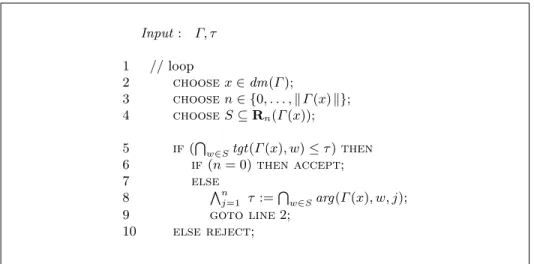
The variable τ holds the value of the current inhabitation goal, processed as follows. First, values for x, n and S are existentially generated (lines 2–4). It is then tested (line 5) that the current goal type τ is a supertype of the target intersection and, if so, the machine transitions to the universal state (line 8).

In every branch of computation created at step 8, the goal τ is set to the ap- propriate argument type, and the computation resumes again from line 2. The computation stops when there is no arguments to process (line 6).

Theorem 12. The inhabitation problem in fcl (∩, ≤) is Exptime -complete.

Proof. Inhabitation remains Exptime -hard in the presence of subtyping, and the proof remains essentially the same. Therefore it is omitted, see [16] for details.

Membership in Exptime follows from the fact that the Turing machine M

shown in Figure 4 solves the inhabitation problem in alternating polynomial

Input : Γ, τ 1 // loop

2 choose x ∈ dm(Γ );

3 choose n ∈ {0, . . . , kΓ (x) k};

4 choose S ⊆ R

(Γ (x));

5 if ( T

w∈S

tgt(Γ (x), w) ≤ τ ) then 6 if (n = 0) then accept ;

7 else

8 V

j=1

τ := T

w∈S

arg(Γ (x), w, j);

9 goto line 2;

10 else reject ;

Fig. 4: Alternating Turing machine M deciding inhabitation for fcl (∩, ≤)

space. Correctness (the machine accepts (Γ, τ) iff Γ ` e : τ for some e) follows easily from Lemma 10 (the machine is a direct implementation of the lemma).

To see that the machine is polynomial space bounded, notice that the variable S holds a subset of R

for n ≤ k Γ k, hence it consumes memory linear in the size of the input. Moreover, Lemma 8 shows that the subtyping relation is decidable in polynomial time (and space). Finally, notice that the variable τ holds types that are intersections of distinct strict subterms of the type Γ (x), and there is

only a linear number of subterms. u t

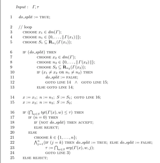
Uniqueness of inhabitation with subtyping. In order to show that uniqueness of inhabitation in system fcl (∩, ≤) is in Exptime we modify the inhabitation algorithm using alternation to search for more than one inhabitant. Figure 5 shows an alternating polynomial space Turing machine accepting Γ and τ if and only if there exists more than one inhabitant e with Γ ` e : τ in system fcl (∩, ≤). In this machine, alternation is used in two different ways, to search for inhabitants of argument types (as was already done in Figure 4) as well as to search for two different inhabitants. The machine solves the ambiguity problem (given Γ, τ, does there exist more than one term e with Γ ` e : τ ?) by nondeterministically guessing an inhabitant (lines 3–5) and a point from which another inhabitant can be “split” off (lines 6–9). See [16] for full details.

Theorem 13. In system fcl (∩, ≤), uniqueness of inhabitation is in Exptime . Finiteness of inhabitation with subtyping Lemma 10 (Path Lemma) yields an alternative proof system for fcl (∩, ≤), consisting only of the following rule schema (P), where S ⊆ R

(Γ (x)):

Γ `

e

: T

w∈S

arg(Γ (x), w, j) (j = 1, . . . , n) T

w∈S

tgt(Γ (x), w) ≤ τ

Γ `

@

(x, e

, . . . , e

) : τ (P)

Input : Γ, τ 1 do split := true ; 2 // loop

3 choose x

∈ dm (Γ );

4 choose n

∈ {0, . . . , k Γ (x

) k};

5 choose S

⊆ R

(Γ (x

));

6 if (do split) then

7 choose x

∈ dm (Γ );

8 choose n

∈ {0, . . . , kΓ (x

) k};

9 choose S

⊆ R

(Γ (x

));

10 if (x

6= x

or n

6= n

) then 11 do split := false ;

12 goto line 14 ∧ goto line 15;

13 else goto line 14;

14 x := x

; n := n

; S := S

; goto line 16;

15 x := x

; n := n

; S := S

; 16 if ( T

w∈S

tgt(Γ (x), w) ≤ τ ) then 17 if (n = 0) then

18 if ( not do split) then accept ; 19 else reject ;

20 else

21 choose k ∈ {1, . . . , n};

22 V

j=1

( if (j = k) then do split := true ; else do split := false ;

23 τ := T

w∈S

arg(Γ (x), w, j);

24 goto line 3)

25 else reject ;

Fig. 5: Alternating Turing machine deciding ambiguity of inhabitation

Type judgements derivable by (P) are written as Γ `

e : τ. Notice that rule (P) becomes an axiom scheme when n = 0.

Lemma 14. Γ ` (x e

. . . e

) : τ if and only if Γ `

@

(x, e

, . . . , e

) : τ.

Proof. Immediate by induction using Lemma 10. u t

Clearly, a proof Π of Γ `

e : τ assigns a type to every subterm e

of e, applying rule (P), with some set S. If e

= @

(x, e

, . . . , e

) then the triple (x, n, S) is called the Π -stamp at e. We say that a proof Π of Γ `

e : τ is cyclic , if there is a subterm e

of e and a proper subterm e

of e

have the same Π -stamp.

Lemma 15. Let Π be a proof of Γ `

e : τ. If the depth of e exceeds |Γ | · 2

·

|dm(Γ )| then the proof Π is cyclic.

Lemma 16. There are infinitely many inhabitants e with Γ ` e : τ if and only if there exists a cyclic proof of Γ `

e

: τ for some e

.

Theorem 17. In system fcl (∩, ≤), finiteness of inhabitation is in Exptime . Proof. Consider the algorithm shown in Figure 6. It is an alternating polynomial space Turing machine accepting Γ and σ if and only if there exists an inhabi- tant e with a cyclic proof of Γ `

e : σ. By Lemma 16, therefore, infiniteness of inhabitation is in Exptime for system fcl (∩, ≤), and hence finiteness of inhab- itation is in Exptime . Full details can be found in [16]. u t

Input : Γ, τ 1 count := 0;

2 inf := true ; 3 choose y ∈ dm (Γ );

4 choose m ∈ {0, . . . k Γ (y)k};

5 choose Q ⊆ R

(Γ (y));

6 // loop

7 choose x ∈ dm(Γ );

8 choose n ∈ {0, . . . , kΓ (x) k};

9 choose S ⊆ R

(Γ (x));

10 if (inf and (x, n, S) = (y, m, Q)) then count := count + 1;

11 if ( T

w∈S

tgt(Γ (x), w) ≤ τ ) then 12 if (n = 0) then

13 if (inf ) then

14 if (count = 2) then accept else reject ;

15 else accept

16 else

17 choose k ∈ {1, . . . , n};

18 V

j=1

( if (j = k) then inf := true else inf := false ;

20 τ := T

w∈S

arg(Γ (x), w, j);

21 goto line 7)

22 else reject ;

Fig. 6: Alternating Turing machine deciding infiniteness of inhabitation

Acknowledgement The authors thank Boris D¨ udder and Moritz Martens for

helpful comments.

References

1. H. Barendregt, M. Coppo, and M. Dezani-Ciancaglini. A filter lambda model and the completeness of type assignment. Journal of Symbolic Logic, 48(4):931–940, 1983.

2. Ch. Ben-Yelles. Type Assignment in the Lambda-Calculus: Syntax and Seman- tics. PhD thesis, Department of Pure Mathematics, University College of Swansea, September 1979.

3. M. Coppo and M. Dezani-Ciancaglini. An extension of basic functionality theory for lambda-calculus. Notre Dame Journal of Formal Logic, 21:685–693, 1980.

4. M. Dezani-Ciancaglini and R. Hindley. Intersection types for combinatory logic.

Theoretical Computer Science, 100(2):303–324, 1992.

5. H. Comon et al. Tree Automata Techniques and Applications. Available online at http://tata.gforge.inria.fr, November 18, 2008.

6. J. R. Hindley. The simple semantics for Coppo-Dezani-Sall´ e types. In International Symposium on Programming, volume 137 of LNCS, pages 212–226. Springer, 1982.

7. Naoki Kobayashi and C.-H. Luke Ong. A type system equivalent to the modal mu-calculus model checking of higher-order recursion schemes. In LICS, pages 179–188. IEEE Computer Society, 2009.

8. M. Kozik. A finite set of functions with an E xptime -complete composition prob- lem. Theoretical Computer Science, 407:330–341, 2008.

9. T. Kurata and M. Takahashi. Decidable properties of intersection type systems.

In TLCA, volume 902 of LNCS, pages 297–311. Springer, 1995.

10. Dariusz Ku´ smierek. The inhabitation problem for rank two intersection types. In TLCA, volume 4583 of LNCS, pages 240–254. Springer, 2007.

11. D. Leivant. Polymorphic type inference. In Proc. 10th ACM Symp. on Principles of Programming Languages, pages 88–98. ACM, January 1983.

12. Y. Lustig and M. Y. Vardi. Synthesis from component libraries. In FOSSACS, volume 5504 of LNCS, pages 395–409. Springer, 2009.

13. Mayur Naik and Jens Palsberg. A type system equivalent to a model checker. In ESOP, volume 3444 of LNCS, pages 374–388. Springer, 2005.

14. Ch. H. Papadimitriou. Computational Complexity. Addison-Wesley, 1994.

15. G. Pottinger. A type assignment for the strongly normalizable lambda-terms. In J. Hindley and J. Seldin, editors, To H. B. Curry: Essays on Combinatory Logic, Lambda Calculus and Formalism, pages 561–577. Academic Press, 1980.

16. J. Rehof and P. Urzyczyn. Finite combinatory logic with intersection types. Tech- nical Report 834, Dept. of Computer Science, Technical University of Dortmund, http://ls14-www.cs.tu-dortmund.de/index.php/Datei:TR-834.pdf, 2011.

17. S. Salvati. Recognizability in the simply typed lambda-calculus. In WoLLIC, volume 5514 of LNCS, pages 48–60. Springer, 2009.

18. P. Urzyczyn. The emptiness problem for intersection types. Journal of Symbolic Logic, 64(3):1195–1215, 1999.

19. P. Urzyczyn. Inhabitation of low-rank intersection types. In TLCA, volume 5608 of LNCS, pages 356–370. Springer, 2009.

20. P. Urzyczyn. The logic of persistent intersection. Fundamenta Informaticae, 103:303–322, 2010.

21. B. Venneri. Intersection types as logical formulae. Journal of Logic and Computa- tion, 4(2):109–124, 1994.

22. J. B. Wells and B. Yakobowski. Graph-based proof counting and enumeration with applications for program fragment synthesis. In LOPSTR, volume 3573, pages 262–

277. Springer, 2005.