A Simple and Successful Shrinkage Method for Weighting Estimators of Treatment Effects

IHS Economics Series Working Paper 304

September 2014

A Simple and Successful Shrinkage Method for Weighting Estimators of Treatment Effects

Winfried Pohlmeier

Ruben Seiberlich

S. Derya Uysal

Impressum Author(s):

Winfried Pohlmeier, Ruben Seiberlich, S. Derya Uysal Title:

A Simple and Successful Shrinkage Method for Weighting Estimators of Treatment Effects

ISSN: Unspecified

2014 Institut für Höhere Studien - Institute for Advanced Studies (IHS) Josefstädter Straße 39, A-1080 Wien

E-Mail: o ce@ihs.ac.at ffi Web: ww w .ihs.ac. a t

All IHS Working Papers are available online: http://irihs. ihs. ac.at/view/ihs_series/

This paper is available for download without charge at:

https://irihs.ihs.ac.at/id/eprint/2891/

A Simple and Successful Shrinkage Method for Weighting Estimators of Treatment Effects

Winfried Pohlmeier ¹ , Ruben Seiberlich ¹ and Selver Derya Uysal ²

1

University of Konstanz

2

Institute for Advanced Studies, Vienna

September 2014

All IHS Working Papers in Economics are available online:

https://www.ihs.ac.at/library/publications/ihs-series/

Economics Series

Working Paper No. 304

A Simple and Successful Shrinkage Method for Weighting Estimators of Treatment Effects ^✩

Winfried Pohlmeier ^a , Ruben Seiberlich ^a , Selver Derya Uysal ^{b, ∗}

a

University of Konstanz, Department of Economics, Konstanz, Germany

b

IHS, Department of Economics and Finance,Vienna, Austria

Abstract

A simple shrinkage method is proposed to improve the performance of weighting estimators of the average treatment effect. As the weights in these estimators can become arbitrarily large for the propensity scores close to the boundaries, three dif- ferent variants of a shrinkage method for the propensity scores are analyzed. The results of a comprehensive Monte Carlo study demonstrate that this simple method substantially reduces the mean squared error of the estimators in finite samples, and is superior to several popular trimming approaches over a wide range of settings.

Keywords:

Average treatment effect, econometric evaluation, penalizing, propensity score, shrinkage

1. Introduction

In this paper, we introduce a simple way of improving propensity score weighting and doubly robust estimators in terms of the mean squared error (MSE) in finite samples. Our approach achieves a lower MSE by shrinking the propensity score

✩

The supplementary Web Appendix for additional results is available online at http://elaine.ihs.ac.at/~uysal/webappendix_SYW.pdf.

∗

Correspondence to: IHS, Vienna, Stumpergasse 56, A-1060, Vienna, Austria. Tel.:+43 1 59991 156

Email address: uysal@ihs.ac.at (Selver Derya Uysal)

towards the share of treated. This James-Stein type simple shrinkage substantially mitigates the problems arising from propensity score estimates close to the bound- aries. It further reduces the variance of the weights and, therefore, the variance of the average treatment effect (ATE) estimators based on propensity score weighting.

We find that the proposed shrinkage method is a successful alternative to the popu- lar trimming methods. “Trimming,” here, refers to the act of dropping observations with propensity scores that are too high or too low. Different trimming methods offer different ways of determining the threshold for the extremes. We show that our approach can be used in a complementary fashion to trimming by applying shrinkage in a first step, and then trimming the shrunken estimates of the propensity scores so that fewer observations will be disregarded by trimming.

Even though shrinkage methods are very popular in other fields of statistics and econometrics, they have not yet been combined with weighting estimators. A no- table exception is Fr¨olich (2004). He applies ridging for local polynomial estimators (Seifert and Gasser, 1996) to matching estimators of the average treatment effect on the treated, in order to overcome the problems of estimating nonparametric models when the conditional variance is unbounded. Our proposed shrinkage method relies on a linear combination of the conditional and unconditional mean of the treatment variable. As in other shrinkage methods, the degree of shrinkage is determined by a tuning parameter. We propose three different methods for choosing this parame- ter. All three of our methods provide consistent estimates of the propensity score;

they differ in their computational burdens and their underlying reasoning. The first method relies on a fixed valued tuning parameter, which depends only on the sam- ple size and vanishes asymptotically. The tuning parameter of the second method is based on the MSE minimization of the propensity score, while for the third method, the optimal tuning parameter is derived by means of cross-validation.

We demonstrate the MSE gains in finite samples through a comprehensive Monte

Carlo study. To make our results comparable, we design our Monte Carlo study

as in the settings of Busso et al. (2009) for poor overlap of control and treatment

groups. Busso et al. (2009) propose these settings to replicate those of the earlier study by Fr¨olich (2004). We construct 72 settings to capture several possible issues when estimating the treatment effects, and we consider homogeneous and hetero- geneous treatment, homoscedastic and heteroscedastic errors, as well as different ratios of treated and control group. Our simulation design, further, captures differ- ent functional forms. Since the shrunken propensity scores are constructed in such a way that they converge to the conventional propensity scores, our proposed method is asymptotically equivalent to the standard approaches without shrinkage. This is why we focus only on sample sizes of 100, 200 and 500. Furthermore, we evaluate the finite sample performance of shrinkage in combination with several trimming rules.

Busso et al. (2009) consider only one regressor in their Monte Carlo studies. We additionally carry out a Monte Carlo study with a larger set of regressors for all 72 settings. Our results show that weighting estimators based on shrunken propensity scores have lower MSE than all other competitors in almost all settings.

The paper is organized as follows. Section 2 reviews the estimation methods and trimming rules. Section 3 introduces the shrunken propensity score and the methods for choosing the tuning parameter. In Section 4, we present the design and the results of the Monte Carlo study in detail. Section 5 concludes the paper.

2. Propensity Score Methods

2.1. Estimation of ATE

Consider the case of a binary treatment within Rubin’s (1974) potential outcome

model. Let Y 1i and Y 0i be the two potential outcomes for person i if she takes

the treatment and if she does not, respectively. D _i denotes the binary treatment

indicator indicating whether person i participates in the program (D i = 1) or not

(D i = 0). The observed outcome variable, Y i , can then be written as a function of

potential outcomes and the treatment variable as follows:

Y i = D i Y 1i + (1 − D i )Y 0i , for i = 1, . . . , n. (1) The difference between two potential outcomes of an individual, Y 1i − Y 0i , denotes the individual’s treatment effect. Depending on the realized treatment status, we observe only one of these two potential outcomes. Hence, the individual treatment effect cannot be identified from observed data. Under certain assumptions, however, we can still identify various average treatment effects. In this paper, we focus on the average treatment effect (ATE), defined as

∆ ATE = E[Y 1i − Y 0i ], (2)

which measures the expected treatment effect if individuals are randomly assigned to treatment and control groups.

The identification of the ATE depends on two crucial assumptions. The first one is that, conditional on confounding variables, the potential outcomes are stochastically independent of the treatment: Y 0i , Y 1i ⊥ D i | X i , where X i denotes the observable con- founding variables of individual i. This assumption, known as the unconfoundedness assumption, requires that all confounding factors associated with the potential out- comes as well as the participation decision are observed. If the unconfoundedness assumption is satisfied, various estimation methods (e.g. weighting, regression, and matching methods) can be used to estimate the ATE.

The second assumption is the overlap assumption. It requires that the propensity score lies strictly between zero and one. In other words, each unit in a defined population has a positive probability of being treated and of not being treated. Al- though this type of overlap assumption is standard in the literature (see, for example, Rosenbaum and Rubin, 1983; Heckman et al., 1997; Hahn, 1998; Wooldridge, 2002;

Imbens, 2004), there is a stronger version of the overlap assumption called “strict

overlap” (see Robins et al., 1994; Abadie and Imbens, 2006; Crump et al., 2009).

Strict overlap requires that the probability of being treated is strictly between ξ and 1 − ξ for some ξ > 0. Khan and Tamer (2010) point out that another assumption comparable to the strict overlap assumption is needed for √

n-convergence of some semiparametric estimators.

The number of studies investigating the effect of violations of the overlap assump- tion on the properties of treatment effect estimators in finite samples is rather lim- ited. Notable exceptions are Busso et al. (2009), and more recently, Lechner and Strittmatter (2014) who examine the effect of this type of violations for a number of semiparametric and parametric treatment effect estimators. We discuss the em- pirical trimming methods to estimate an overlap region in the following subsection.

Under the assumptions listed above, the ATE can be identified and estimated. Sev- eral estimation methods are proposed in the literature. Here we focus only on the methods which use the propensity scores as weights. The propensity score, i.e., the probability of being treated conditional on the characteristics X i , is given by

p _i = Pr [D _i = 1 | X _i ] = p(X _i ). (3) As the propensity score is an unknown probability, it needs to be estimated. Con- ventionally, standard parametric maximum likelihood methods are used to obtain the estimated propensity score denoted by ˆ p i .

Following Busso et al. (2009), we formulate the weighting type estimator for the ATE as follows:

∆ ˆ AT E = 1 n 1

n

X

i=1

D i Y i ω ˆ i1 − 1 n 0

n

X

i=1

(1 − D i )Y i ω ˆ i0 , (4)

where n 1 is the number of treated observations and n 0 is the number of controls.

ˆ

ω i0 and ˆ ω i1 are defined differently for different types of weighting estimators. Here,

we consider three inverse probability weighting schemes proposed in the literature.

The first one, which we can call IPW1, uses the following weighting functions ˆ

ω _i0 ⁽¹⁾ = n 0

n

. (1 − p ˆ i ) (5) ˆ

ω _i1 ⁽¹⁾ = n 1

n

. p ˆ i , (6)

where n = n 0 + n 1 is the total number of observations.

The second weighting function, IPW2, results from an adjustment to force the weights to add up to one (Imbens, 2004). Formally, the weights are given by

ˆ

ω _i0 ⁽²⁾ = 1 1 − p ˆ i

. 1 n 0

n

X

i=1

1 − D i

1 − p ˆ i

(7) ˆ

ω _i1 ⁽²⁾ = 1 ˆ p i

. 1 n 1

n

X

i=1

D i

ˆ p i

. (8)

The third weighting function, IPW3, which is not so common in the literature, is a combination of the first two methods, where the asymptotic variance of the resulting estimator is minimized for a known propensity score (see Lunceford and Davidian, 2004, for details). The weights are given by

ˆ

ω _i0 ⁽³⁾ = ₁₋ ¹ _{p ˆ}

i

(1 − C i0 ) .

1 n

P n i=1

(1−D

)

1−ˆ p

(1 − C i0 ) (9)

ˆ

ω _i1 ⁽³⁾ = _p ¹ _ˆ

i

(1 − C i1 ) .

1 n

P n i=1

D

ˆ

p

(1 − C i1 ), (10)

with

C i0 =

1 1 − p ˆ

1 n

P n i=1

1 − D

1 − p ˆ

p ˆ i − D i

1 n

P n i=1

1−D

1 − p ˆ

p ˆ i − D i

2 (11)

C _i1 =

1 ˆ p

1 n

P n i=1

D

ˆ

p

(1 − p ˆ i ) − (1 − D i )

1 n

P n i=1

D

ˆ

p

(1 − p ˆ i ) − (1 − D i ) 2 . (12)

In all three cases, ˆ ω i0 depends on _1−ˆ ¹ _p

i

and ˆ ω i1 on _{p ˆ} ¹

i

. As the estimated propensity

score for individual i from the control group approaches one, the weight for individual

i dominates the weights of all other observations. This also holds if the estimated propensity score of an individual from the treatment group is close to zero. In that case, ˆ ω i1 becomes very large, again leading to an ATE estimator that exhibits a large variance.

We also consider the doubly robust (DR) estimator of the ATE derived from a weighted regression of the outcome model where the weights are inversely related to the propensity scores. The advantage of the doubly robust estimator is that it stays consistent even if the outcome model or the propensity score model is misspec- ified, but not both. For different types of doubly robust methods, see Robins and Rotnitzky (1995), Wooldridge (2007), Tan (2006), and Uysal (2014), among others.

In this paper, we consider the doubly robust method used by Hirano and Imbens (2001). They estimate the ATE using a weighted least squares regression of the following outcome model with weights based on Eq. (5). The outcome model is

Y i = α 0 + ∆ AT E D i + X _i ^′ α 1 + D i (X i − X) ¯ ^′ α 2 + ε i (13) ˆ

ω _i ^dr = s D i

ˆ p i

+ 1 − D i

1 − p ˆ i

, (14)

where ¯ X is the sample average of X _i . The weight ˆ ω _i ^dr again depends on _1−ˆ ¹ _p

i

and _{p ˆ} ¹

i

, hence propensity scores close to one or zero affect the doubly robust estimator, just as they do for the weighting estimators above.

2.2. Trimming Rules

A major drawback of the weighting and the doubly robust estimators is that they

can vary greatly if the weights of some observations are very large. As mentioned

before, for the ATE this can be the case when the propensity score is close to one or

zero. In empirical studies, it is standard to trim the estimated propensity score in

order to mitigate the problems that arise when propensity scores are too extreme.

A trimming rule determines an upper and a lower limit for the propensity score.

Observations with propensity scores outside of the chosen limits are dropped from the estimation sample to sustain the overlap assumption. From the various trimming rules proposed in the literature, we consider the three trimming rules which are most frequently used in empirical studies. These trimming rules are applied as follows:

TR1. The first trimming rule goes back to a suggestion by Dehejia and Wahba (1999). Let T _i ^{AT E} = 1l (ˆ a < p ˆ i < ˆ b), where ˆ b is the m ^th largest propensity score in the control group and ˆ a the m ^th smallest propensity score in the treatment group. Then the estimators are computed based on the subsample for which T _i ^{AT E} = 1.

TR2. In the second trimming rule, suggested by Crump et al. (2009), all units with an estimated propensity score outside the interval [0.1; 0.9] are discarded.

TR3. The third trimming method, suggested by Imbens (2004), is setting an upper bound on the relative weight of each unit.

In Busso et al. (2009), the first two rules perform best. The third one is shown to perform decently in Huber et al. (2013). Note that the third rule restricts the weights, and not the propensity scores directly. The loss of information and the loss of efficiency due to the dropped observations is an obvious problem implied by the application of trimming rules. The shrinkage method we propose in this paper – alone or in combination with trimming rules – mitigates this problem.

3. Shrunken Propensity Score

We propose three simple variants on the James-Stein shrinkage method for the propensity score. These stabilize the treatment effect estimators by shrinking the propensity scores away from the boundaries.

The basic idea is to shrink the estimated propensity score, ˆ p i , towards the estimated

unconditional mean, ¯ D = ˆ E[D _i = 1] = _n ¹ P n

i D _i , as given below ˆ

p ^s _i = 1 − λ i (n) ˆ

p i + λ i (n) ¯ D, (15)

where 0 ≤ λ i (n) ≤ 1 is a tuning parameter that depends on the sample size. Eq.

(15) implies that our proposed shrunken propensity score is always closer to the share of treated and, therefore, the shrunken propensity scores have a lower variance than the conventional propensity scores. This enables us to estimate the treatment effects with a lower MSE.

Shrinking towards the unconditional mean prevents the propensity scores estimates from being close to one or zero. In contrast to trimming rules, where some obser- vations are dropped if their propensity scores are too high or too low, shrinkage pushes the estimated propensity score away from the boundaries, leading to stabi- lized weights without information reduction and without reducing the sample size.

As we are interested in improving the small sample performance of weighting and doubly robust estimators, we propose to choose λ i (n) such that the penalty vanishes asymptotically. For λ i (n) = O (n ^−δ ) with δ > 0, the shrinkage estimator ˆ p ^s _i consis- tently estimates the true propensity score. For δ > 1/2, ˆ p ^s _i has the same limiting distribution as the conventional propensity score ˆ p i given by

√ n(ˆ p ^s _i − p i ) = √

n(ˆ p i − p i ) + Op (1),

and for δ = 1/2, the limiting distribution is biased. In the following, we consider three alternative methods of choosing λ i (n). All three provide consistent estimates of the propensity score.

Method 1: Fixed Tuning Parameter Method

This method is based on a single tuning parameter of the form λ _i (n) = _n ^c

. For

δ = 1/2 the parameter c determines the asymptotic bias. The limiting distribution

of ˆ p ^s _i is given by

√ n(ˆ p ^s _i − p i ) −→ N ^d ∆, Ω , where ∆ = c E[D i ] − p i

denotes the asymptotic bias. Note that for a given sample size, Method 1 is equivalent to a fixed tuning parameter approach, i.e., the pa- rameters c and δ solely determine the nature of the asymptotic distribution of the shrunken propensity score estimates. For given values of c and δ, this method is easy to implement with basically no computational cost, but is not optimized with respect to any criterion.

Method 2: MSE Minimizing Tuning Parameter Method

In Method 2, the tuning parameter λ i (n) is determined by minimizing the MSE of the shrunken propensity score, MSE(ˆ p ^s _i ), in (15). Assuming E [ˆ p i ] ≈ p i , the optimal λ i (n) is given by

λ ^∗ _i (n) = V [ˆ p i ] − Cov(ˆ p i , D) ¯

V [ˆ p _i ] + ^E[D

^](1 _n ^{− E[D}

^]) + (E [D _i ] − E [ˆ p _i ]) ² − 2 Cov(ˆ p _i , D) ¯ . (16) Since λ ^∗ _i (n) depends on unknown parameters, we replace the squared bias, variance, and covariances with their bootstrap estimates. Like the tuning parameter in the first method, the MSE(ˆ p ^s _i )-minimizing tuning parameter (16) converges to zero as the sample size increases. Note that the latter method yields optimal λs for each observation in the sample. Observation-specific tuning parameters, however, create considerable estimation noise. We therefore propose to stabilize the estimates by using the mean of MSE(ˆ p ^s _i )-minimizing tuning parameter, ¯ λ ^∗ (n) = _n ¹ P n

i=1 λ ^∗ _i (n).

An alternative would be to choose λ such that the MSE of the vector of the shrunken

propensity scores is minimized. (The results derived from this are comparable to

those obtained by using ¯ λ ^∗ (n), and are available upon request.) Averaging has the

further advantage that it preserves the ordering of the propensity scores.

Method 3: Cross-Validated Tuning Parameter Method

In the third method, λ is chosen by means of cross-validation. The idea is to minimize the mean squared prediction error of the estimated propensity score with respect to λ. The mean squared prediction error is calculated by leave-one-out cross-validation for each λ in an equally spaced grid of k + 1 λs, i.e. [0, λ ₍₁₎ , . . . , λ _(k−1) , 1]. The optimal λ ^∗ _cv is given by the value of λ in the grid yielding the smallest cross-validated mean squared prediction error. Cross-validating λ with Method 3 is equivalent to optimizing the bias parameter c for a given δ, i.e., c ^∗ _cv = λ ^∗ _cv n ^δ .

4. Monte Carlo Study

4.1. Simulation Design

We demonstrate the efficiency gains due to propensity score shrinkage through a comprehensive Monte Carlo study. We base our simulation design on Busso et al.

(2009) so that our results are comparable with theirs. Since our approach shrinks the propensity score towards the share of the treated, it is especially valuable in situations where the overlap is fulfilled but the strict overlap assumption is not.

Therefore, in the following, we concentrate on those designs of Busso et al. (2009) which are not consistent with the strict overlap assumption. When the strict overlap condition is also fulfilled, our approach improves the MSE of the different estimators as well, but due to space constraints the results are not discussed here. For the simulation study, D i and Y i are generated as follows

D i = 1l { η + X _i ^′ κ − u i > 0 } (17)

Y i = D i + m(p(X i )) + γD i m(p(X i )) + ε i , (18)

where the error terms u i and ε i are independent of each other. We firstly use a

scalar confounding variable, X _i , assuming a standard normally distributed random

variable as in Busso et al. (2009) and a corresponding one-dimensional parameter κ.

Next, we use a high-dimensional covariate vector X _i and a conformable coefficient vector for our simulations. m( · ) is a function of the propensity score. We use two different functions in the Monte Carlo study given in Table 1.

Table 1: Functional form for m(q)

m(q) Formula Description

m

(q) 0.15 + 0.7q Linear

m

(q) 0.2 + √ 1 − q − 0.6(0.9 − q)

Nonlinear

The error term, u i , is drawn from a standard normal distribution, so the propensity score function is

p(X i ) = Φ(η + X _i ^′ κ). (19)

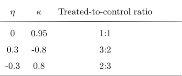
We generate various treated-to-control ratios by choosing three different combina- tions of η and κ. Table 2 summarizes the parameter values and resulting ratios for a scalar X i . Figure A.1 in the Appendix presents smoothed histograms of the propen- sity scores as in Busso et al. (2009) for all three treated-to-control ratios. The plots indicate that our DGP with a scalar X i leads to high density mass at the boundaries for all ratios, which in turn will result in overlap problems in finite samples.

Table 2: Treated-to-control ratios η κ Treated-to-control ratio

0 0.95 1:1

0.3 -0.8 3:2

-0.3 0.8 2:3

The error term in the outcome equation, ε i , is specified as

ε i = ψ(e i p(X i ) + e i D i ) + (1 − ψ)e i , (20)

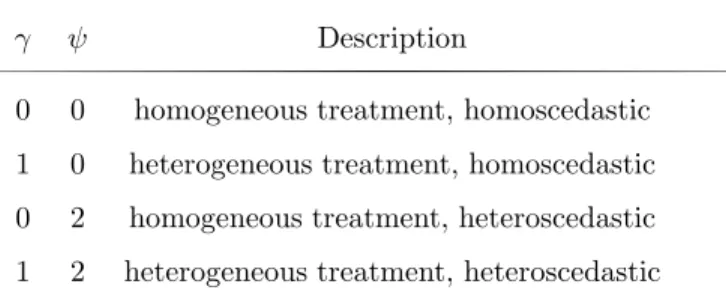
where e _i is an i.i.d. standard normal random variable and ψ is a parameter control- ling for heteroscedasticity. In other words, for ψ = 0, ε i is a homoscedastic error term, and if ψ 6 = 0, ε i is heteroscedastic. We specify whether the treatment effect is homogeneous or not by choosing different values of γ in Eq. (18). Treatment homogeneity implies that the treatment effect does not vary with different X i ’s. In this case, the causal treatment effect is the same for all individuals. Like Busso et al. (2009), we use various combinations of ψ and γ , given in Table 3, to create four different settings.

Table 3: Parameter combinations

γ ψ Description

0 0 homogeneous treatment, homoscedastic 1 0 heterogeneous treatment, homoscedastic 0 2 homogeneous treatment, heteroscedastic 1 2 heterogeneous treatment, heteroscedastic

Our simulations are based on 10,000, 5,000 and 2,000 Monte Carlo samples for

sample sizes n = 100, 200 and 500, respectively. The choice of making the number of

replications inversely proportional to the sample size is motivated by the fact that

simulation noise depends negatively on the number of replications and positively

on the variance of the estimators, which depends negatively on the chosen sample

size. Hence, the simulation noise is constant if the Monte Carlo samples are chosen

inversely proportional to the sample size (Huber et al., 2013). Our Monte Carlo

study consists of three parts. In the first part, we use the conventional and shrunken

propensity scores without applying any trimming rules. In the second part, we

incorporate the most commonly used trimming rules to the conventional as well as

the shrunken propensity scores. In the last part, we consider a higher dimensional

covariate vector for our simulations. As in Busso et al. (2009), we estimate the ATE

given in Eq. (2) for each possible DGP using all three weighting methods and the

doubly robust method. As suggested by the distribution of the error term, u i , we

obtain ˆ p _i by maximum likelihood probit.

4.2. Shrinkage without Trimming

In a first step, by means of a small Monte Carlo exercise, we provide a reference point for an optimal choice of a λ in terms of the MSE( ˆ ∆ AT E ). For the hypothetical case where the true ATE is known, we choose a λ that minimizes MSE( ˆ ∆ AT E ). Due to the computational burden, we conduct the procedure only for the nonlinear (m 2 (q)), heteroscedastic (ψ = 2), heterogeneous (γ = 1) design with more control units than treated units (η = − 0.3, κ = 0.8), and only for sample size of 100. We apply the following procedure to choose an MSE( ˆ ∆ AT E )-minimizing λ:

1. We draw 10,000 Monte Carlo samples for this specification.

2. For each Monte Carlo sample, we estimate the shrunken propensity scores for λ = 0, 0.01, 0.02, ..., 1 and the ATE by the four methods with each of these shrunken propensity scores.

3. We calculate the MSE of the ATE estimators, ˆ ∆ AT E , over 10,000 Monte Carlo samples for each λ and choose the MSE( ˆ ∆ _{AT E} )-minimizing λ for each method.

4. Steps (1)-(3) are repeated 500 times.

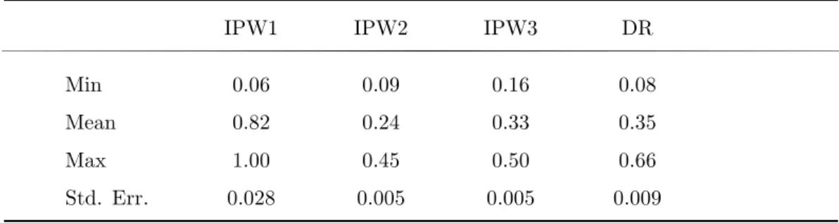
The minimum, mean, maximum and standard error of 500 optimal λs are displayed in Table 4.

Table 4: Descriptive statistics of the MSE( ˆ ∆

)-minimizing λs with known ATE

IPW1 IPW2 IPW3 DR

Min 0.06 0.09 0.16 0.08

Mean 0.82 0.24 0.33 0.35

Max 1.00 0.45 0.50 0.66

Std. Err. 0.028 0.005 0.005 0.009

Note: The MSE( ˆ ∆

)-minimizing λ

s are obtained from a Monte Carlo study for the specification with

n = 100, γ = 1, ψ = 2, η = − 0.3, κ = 0.8 and m

(q) for the hypothetical case with known ATE. We use

10,000 Monte Carlo replications and replicate this procedure 500 times. The descriptive statistics are of 500

The results show that the largest shrinkage is required for IPW1 and the least for IPW2. In all of the 500 replications, λ is never chosen to be equal to zero, which implies that shrinkage is always optimal in terms of MSE( ˆ ∆ AT E ) for this setting and sample size.

For Method 1, the fixed tuning parameter method, we set c = 1 and δ = 1/2, i.e., λ i (n) = 1/ √

n. The value of c = 1 leads to an asymptotic bias equal to the difference between the propensity score and the unconditional treatment probability. Given the results for the MSE( ˆ ∆ AT E )-minimizing λ reported in Table 4, this is a rather conservative value. For the second method, the MSE(ˆ p ^s _i )-minimizing tuning param- eter method, the tuning parameter is computed as the mean over the individual λs given by Eq. (16). For the bootstrap-estimated quantities in Eq. (16), we use 500 bootstrapped replications. For the cross-validation method, the optimal λ is chosen by grid search on an equally spaced grid of 101 λs, i.e., k = 100.

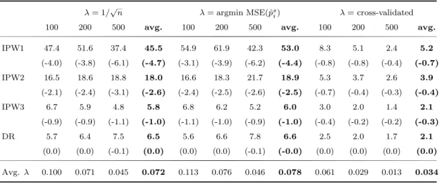
The results for the average improvements across the designs are summarized in Table 5, which has three panels for the three different variants of choosing the tuning pa- rameter λ. The main figures are the average MSE improvements that are due to the shrunken propensity score; they are shown across the designs, for the various estima- tion methods and sample sizes. In addition, the last columns for each method give the average improvement over all sample sizes. Since the MSE can be decomposed into bias and variance components, we also report the percentage change that results from the bias introduced by shrinkage in parentheses,

bias

(ATE(ˆ p))−bias

(ATE(ˆ p

)) bias

(ATE(ˆ p))+Var(ATE(ˆ p))

.

The last row in the same table reports the average λs for each sample and method

of choosing the tuning parameter. For the fixed value λ method, the tuning param-

eter is solely determined by the sample size. For the MSE(ˆ p ^s _i )-minimizing λ and the

cross-validated λ, we obtain different values of λ for every replication. In these cases,

the reported values are average values of λ across different designs and replications

for a given sample size.

Table 5: Shrinkage ATE Estimators: % MSE reductions, averaged across designs

λ = 1/ √

n λ = argmin MSE(ˆ p

) λ = cross-validated

100 200 500 avg. 100 200 500 avg. 100 200 500 avg.

IPW1 47.4 51.6 37.4 45.5 54.9 61.9 42.3 53.0 8.3 5.1 2.4 5.2

(-4.0) (-3.8) (-6.1) (-4.7) (-3.1) (-3.9) (-6.2) (-4.4) (-0.8) (-0.8) (-0.4) (-0.7)

IPW2 16.5 18.6 18.8 18.0 16.6 18.3 21.7 18.9 5.3 3.7 2.6 3.9

(-2.1) (-2.4) (-3.1) (-2.6) (-2.4) (-2.5) (-2.6) (-2.5) (-0.7) (-0.4) (-0.3) (-0.4)

IPW3 6.7 5.9 4.8 5.8 6.8 6.2 5.2 6.0 3.0 2.0 1.4 2.1

(-0.9) (-0.9) (-1.1) (-1.0) (-1.1) (-1.0) (-0.9) (-1.0) (-0.4) (-0.2) (-0.2) (-0.3)

DR 5.7 6.4 7.5 6.5 5.6 6.6 7.8 6.6 2.5 2.0 1.7 2.1

(0.0) (0.0) (-0.1) (0.0) (0.0) (0.0) (-0.1) (-0.0) (0.0) (0.0) (0.0) (0.0) Avg. λ 0.100 0.071 0.045 0.072 0.113 0.076 0.046 0.078 0.061 0.029 0.013 0.034

Note:The average MSE improvements due to the shrunken propensity score for the given method and sample size are reported along with the percentage change which is due to the bias introduced by shrinkage, i.e.,

bias2(ATE( ˆp))−bias2(ATE( ˆps)) bias2(ATE( ˆp))+Var(ATE( ˆp))

(in parentheses).

‘Avg.’ in the last columns for each method refers to the average improvement over all sample sizes.

Table 5 reveals that, regardless of the method of determining λ, the improvements turn out to be more pronounced for IPW1 and IPW2, i.e., for those methods which are most vulnerable to very small or very large propensity scores. This result is es- pecially striking since most estimates in the empirical literature are based on IPW2 (Busso et al., 2009). Using the fixed tuning parameter method, it was possible to improve the MSE of this estimator by an average of 18.0%. This improvement comes at basically no computational costs, due to the simplicity of the linear combination.

The computationally more burdensome MSE(ˆ p ^s _i )-minimizing λ leads to 18.9% im- provement for IPW2. For both choices of λ, the average improvement of IPW3 and DR is still 6.0 to 6.6 %. We see that the improvement is due to a large reduction of the variance, but comes at the expense of introducing a comparatively small bias.

For DR, the increase in the squared bias is nearly zero.

If we compare the average results in Table 5 obtained by the fixed tuning parameter

method to the ones obtained from the MSE(ˆ p ^s _i )-minimization, we find that the latter

yields slightly better results for n = 500. For n = 200 and n = 100, the average

improvements of IPW1 are larger with MSE(ˆ p ^s _i )-minimizing λ, but for the other

estimators, both methods give about the same result. On average, the cross-validated

λ also yields an MSE reduction in all cases, but this method is always dominated by the other two methods of choosing λ.

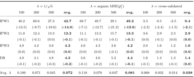
Table 6 provides closer look at the MSE( ˆ ∆ AT E ) improvements for the nonlinear, het- eroscedastic, heterogeneous design. The results of this specific setting are consistent with the average results. Although the improvements are lower than the average re- sults across designs, we still observe considerably high MSE( ˆ ∆ AT E ) improvements, especially with fixed and MSE(ˆ p ^s _i )-minimizing λs.

Table 6: Shrinkage ATE estimators: % MSE reductions for the nonlinear, heteroscedastic, het- erogeneous design

λ = 1/ √ n λ = argmin MSE(ˆ p

) λ = cross-validated

100 200 500 avg. 100 200 500 avg. 100 200 500 avg.

IPW1 40.2 60.6 27.3 42.7 68.7 49.7 29.1 49.2 3.3 0.5 -2.5 0.4

(-12.5) (-9.7) (-19.6) (-14.0) (-7.1) (-12.7) (-21.2) (-13.6) (-2.3) (-2.4) (-1.5) (-2.1)

IPW2 11.0 12.4 13.3 12.2 11.1 13.2 15.7 13.3 3.6 2.9 2.3 2.9

(-0.1) (-0.1) (0.0) (-0.1) (-0.1) (-0.1) (-0.1) (-0.1) (0.0) (-0.1) (0.0) (0.0)

IPW3 4.8 4.2 3.6 4.2 4.6 4.3 3.6 4.2 2.0 1.6 1.2 1.6

(0.0) (0.0) (0.0) (0.0) (0.0) (0.0) (-0.1) (0.0) (0.0) (0.0) (0.0) (0.0)

DR 4.0 4.1 4.8 4.3 3.6 4.6 5.2 4.4 1.6 1.4 1.3 1.4

(-0.1) (-0.2) (-0.3) (-0.2) (-0.1) (-0.2) (-0.1) (-0.1) (-0.1) (0.0) (-0.1) (0.0) Avg. λ 0.100 0.071 0.045 0.072 0.118 0.078 0.047 0.081 0.068 0.032 0.014 0.038

Note: The MSE( ˆ∆AT E) improvements due to the shrunken propensity score for the given method and sample size are reported along with the percentage change which is due to the bias introduced by shrinkage, i.e.,

bias2(ATE( ˆp))−bias2(ATE( ˆps)) bias2(ATE( ˆp))+Var(ATE( ˆp))

, (in parentheses). ‘Avg.’ in the last columns for each method refers to the average improvement over all sample sizes. Simulation for the specification withγ= 1,ψ= 2, η=−0.3,κ= 0.8 andm2(q).

The results for all the other designs are given in Tables A.1-A.3 of the Web Appendix.

Tables A.1 and A.2 show that, in all 288 cases, the use of shrunken propensity

scores leads to an improvement of the MSE of the ATE if the fixed value of λ or

the MSE(ˆ p ^s _i )-minimizing λ is chosen. Table A.3 shows that the use of the shrunken

propensity score leads to an improvement in 99.3% of the MSE comparisons if the

cross-validated λ is taken. In some cases, the improvements can be very substantial

and reach a maximum reduction of 67.7% (for the fixed value λ), 86.9% (for the

MSE(ˆ p ^s _i )-minλ) and 13.8 % (for the cross-validated λ).

4.3. Shrinkage with Trimming

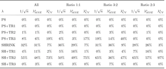
Again we estimate the propensity scores using a probit model and shrink it with the λs chosen by the three different methods we propose. But in contrast to the Monte Carlo simulations in the previous part, we now additionally apply the three trimming rules to the conventional propensity score and to the shrunken propensity scores, before estimating the ATE with weighting and doubly robust methods. For the application of TR1, we set m = 1, and for TR3, we restrict the maximum relative weight to be 4%, as in Huber et al. (2013). Note that applying the trimming rules to the shrunken propensity score leads to a smaller reduction of the effective sample size, since fewer observations lie outside the limits of the two trimming rules after shrinkage. All in all, we have eight possible methods to construct the weights. Table 7 presents the percentage of times a particular method delivers the best estimator in terms of MSE( ˆ ∆ AT E ) for all three methods of choosing the tuning parameter. A very striking finding is that shrinkage combined with trimming rule 2 (SH+TR2) dominates all the other methods, especially when the proportion of the control group is larger than that of the treatment group, regardless of how λ is chosen.

Neither alone nor in combination with TR1 can the conventional propensity score

approach outperform the other methods in terms of MSE. Moreover, shrinkage alone

performs best more often than shrinkage combined with TR1. The pure shrinkage

strategy turns out to be the second best estimation strategy after shrinkage com-

bined with TR2, except when the λ is cross-validated. For the cross-validated λ,

conventional propensity score combined with TR3 takes second place.

Table 7: Frequencies of MSE( ˆ ∆

)-minimizing ATE estimators

All Ratio 1:1 Ratio 3:2 Ratio 2:3

λ 1/ √ n λ

λ

1/ √ n λ

λ

1/ √ n λ

λ

1/ √ n λ

λ

PS 0% 0% 0% 0% 0% 0% 0% 0% 0% 0% 0% 0%

PS+TR1 0% 0% 0% 0% 0% 0% 0% 0% 0% 0% 0% 0%

PS+TR2 1% 1% 0% 2% 0% 0% 0% 3% 0% 0% 1% 0%

PS+TR3 8% 6% 19% 6% 3% 17% 19% 14% 40% 0% 0% 0%

SHRINK 32% 31% 7% 36% 29% 7% 31% 36% 9% 28% 26% 3%

SH+TR1 4% 11% 2% 5% 16% 1% 0% 3% 4% 7% 16% 0%

SH+TR2 55% 48% 73% 50% 49% 75% 65% 36% 47% 65% 57% 97%

SH+TR3 0% 3% 0% 0% 3% 0% 0% 7% 0% 0% 0% 0%

Note: PS: conventional propensity score, TR1: trimming rule 1, TR2: trimming rule 2, TR3: trimming rule 3 and SH: shrinkage. The number in each cell represents the frequency of the corresponding method delivering the minimum MSE with correspondingλ. The first three columns are results among 288 cases for eachλ. Then the results for each treated-to-control ratio is summarized in a similar manner.

Given that shrinkage combined with trimming rule 2 (SH+TR2) outperforms the other methods in most of the cases, we discuss only the comparison of this approach (and not SH+TR1 or SH+TR3) with the ones most frequently used in the literature:

(i) conventional propensity score (PS), (ii) conventional propensity score combined with trimming rule 1 (PS+TR1), (iii) conventional propensity score combined with trimming rule 2 (PS+TR2), and (iv) conventional propensity score combined with trimming rule 3 (PS+TR3). Comparisons of the shrunken propensity score trimmed by other trimming rules with these rules lead to similar but less pronounced results, which we do not present here due to space constraints.

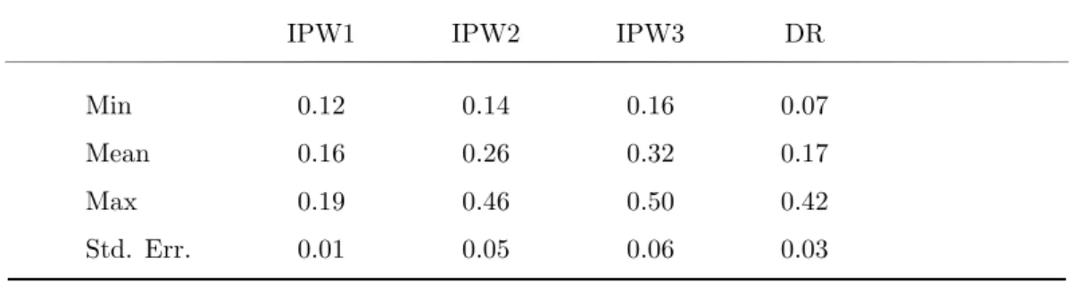
As in the first part, we start with the investigation of MSE( ˆ ∆ _{AT E} )-minimizing λ for

the nonlinear, heteroscedastic, heterogeneous design for the hypothetical case with

known ATE if trimming rule 2 is applied. The results are displayed in Table 8.

Table 8: Descriptive statistics of the MSE( ˆ ∆

)-minimizing λs with known ATE with trimming rule 2 (TR2)

IPW1 IPW2 IPW3 DR

Min 0.12 0.14 0.16 0.07

Mean 0.16 0.26 0.32 0.17

Max 0.19 0.46 0.50 0.42

Std. Err. 0.01 0.05 0.06 0.03

Note: The MSE( ˆ∆_{AT E})-minimizingλ^∗s are obtained from a Monte Carlo study for the specification withn= 100,γ= 1, ψ= 2,η=−0.3,κ= 0.8 andm2(q) for the hypothetical case with known ATE. We use 10,000 Monte Carlo replications and replicate this procedure 500 times. The descriptive statistics are of 500 optimalλs.

In this case, the largest shrinkage is required for IPW3 and the least for IPW1.

Again, in none of the 500 replications do we obtain a value for λ equal to zero. This implies that it is always optimal to have shrinkage in combination with trimming.

If we compare the maximum λs in Table 8 to Table 4, we see that, especially for IPW1, the degree of shrinkage is much smaller if we use trimming rule 2 after shrinking the propensity score. If some kind of trimming is applied, IPW1 shows substantial improvements in terms of MSE. This might be a possible explanation for the decrease in optimal λ for IPW1 if trimming is used. For the IPW2 and IPW3, there is not a big change in optimal λ, because trimming does not lead to such a substantial improvement for these methods.

We summarize the results of the Monte Carlo experiment for each λ choice in Ta-

ble 9. The structure of this table is the same as that of Table 5. Each panel

in Table 9, compares shrinkage combined with trimming rule 2 to one of the four

competitors listed above. Based on the average results in Table 9, the following

general conclusions can be drawn. The average improvements due to SH+TR2 are

ranked as IPW1>IPW2>IPW3>DR when compared to PS, PS+TR1 or PS+TR2

for any λ choice. However, when compared to PS+TR3, the rank order of the aver-

age improvements is IPW2>IPW3>IPW1>DR, and the differences between average

improvements across different estimation methods become smaller.

The average improvements with fixed λ and MSE(ˆ p ^s _i )-minimizing λ are very close,

except in the first row, where the improvements with the latter choice of λ are

slightly higher. The similarity of the results is not surprising because the optimal

λs reported in the last row of Table 9 do not differ much. Note that these values

are smaller than MSE( ˆ ∆ AT E )-minimizing λs for known ATE in Table 8. On aver-

age, the cross-validation method also leads to an improvement in the MSE of the

ATEs for all four estimators. However, we see that shrinkage based on the λs chosen

using the other two methods provide larger average improvements in the MSEs of

the ATEs. Even though the gains are less pronounced, our procedure reduces the

variance and leads to a lower squared bias for all four estimators and all sample

sizes on average. When SH+TR2 is compared to PS+TR1, PS+TR2 or PS+TR3,

it is evident that the average improvements as well as average λs are decreasing as

the sample size increases for all λ choices. However, if SH+TR2 is compared to PS,

the average MSE improvements increase as the sample size increases for the IPW2,

IPW3 and DR estimators of ATE. No general conclusion can be reached about the

order of the average improvements by sample size for IPW1. If we compare Table

5 (SH vs. PS) to the first panel of Table 9 (SH+TR2 vs. PS), we see that the

average improvements in the latter table are higher for all λ choices. However, the

difference is especially striking for the cross-validated λs which are further away from

MSE( ˆ ∆ AT E )-minimizing λs.

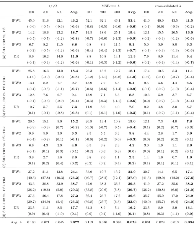
Table 9: Trimmed shrinkage ATE estimators: % MSE reductions, averaged across designs

1/ √

λ MSE-min λ cross-validated λ

100 200 500 Avg. 100 200 500 Avg. 100 200 500 Avg.

(a ) S H + T R 2 v s. P S

IPW1 45.0 51.6 42.1 46.2 52.1 62.1 46.1 53.4 41.0 40.0 43.5 41.5

(-0.6) (-0.5) (-0.6) (-0.6) (-0.8) (-0.5) (-0.6) (-0.6) (-0.1) (0.0) (-0.6) (-0.2)

IPW2 14.2 18.6 23.2 18.7 14.5 18.6 25.1 19.4 12.1 15.5 20.5 16.0

(-0.5) (-0.7) (-1.2) (-0.8) (-0.7) (-0.6) (-1.3) (-0.9) (-0.2) (-0.3) (-1.2) (-0.6)

IPW3 6.7 8.2 11.5 8.8 6.8 8.9 11.5 9.1 5.0 5.9 8.0 6.3

(-0.2) (-0.5) (-1.2) (-0.6) (-0.4) (-0.4) (-1.3) (-0.7) (-0.1) (-0.3) (-1.3) (-0.6)

DR 8.9 10.2 14.0 11.0 8.8 10.8 14.1 11.3 7.9 8.9 11.4 9.4

(-0.1) (-0.4) (-1.2) (-0.6) (-0.1) (-0.3) (-1.2) (-0.6) (-0.2) (-0.4) (-1.4) (-0.7)

(b ) S H + T R 2 v s. P S + T R 1

IPW1 25.8 16.3 13.0 18.4 26.3 15.2 12.7 18.1 17.4 10.5 5.3 11.1

(-1.0) (-0.9) (-0.6) (-0.8) (-1.2) (-1.1) (-0.8) (-1.0) (-0.2) (-0.1) (-0.7) (-0.4)

IPW2 13.1 8.2 7.7 9.7 13.9 7.9 6.3 9.4 9.5 5.6 4.4 6.5

(-0.4) (-0.5) (-1.1) (-0.7) (-0.6) (-0.6) (-1.4) (-0.9) (-0.1) (-0.2) (-1.0) (-0.4)

IPW3 12.8 7.6 6.7 9.1 13.9 7.1 5.3 8.8 10.3 5.9 3.7 6.7

(-0.1) (-0.3) (-0.9) (-0.4) (-0.3) (-0.3) (-1.1) (-0.6) (0.0) (-0.2) (-1.0) (-0.4)

DR 10.7 5.7 5.5 7.3 11.9 5.0 4.0 7.0 9.2 4.8 3.0 5.7

(0.1) (-0.1) (-0.8) (-0.3) (0.1) (-0.1) (-1.0) (-0.3) (0.1) (-0.2) (-1.1) (-0.4)

(c ) S H + T R 2 v s. P S + T R 2

IPW1 20.5 15.1 9.9 15.2 20.9 13.4 10.8 15.0 12.1 7.3 4.0 7.8

(-0.9) (-0.3) (0.7) (-0.2) (-1.0) (-0.7) (0.5) (-0.4) (0.1) (0.2) (0.7) (0.3)

IPW2 9.0 5.9 3.9 6.3 8.5 5.5 3.3 5.8 4.4 2.8 1.7 3.0

(-0.4) (-0.2) (0.1) (-0.1) (-0.6) (-0.2) (0.0) (-0.3) (0.0) (0.2) (0.2) (0.1)

IPW3 6.6 4.3 2.9 4.6 6.5 3.8 2.3 4.2 3.0 1.9 1.1 2.0

(-0.1) (0.1) (0.3) (0.1) (-0.2) (0.0) (0.3) (0.0) (0.0) (0.1) (0.2) (0.1)

DR 3.8 2.7 1.8 2.8 3.8 2.0 1.1 2.3 1.4 1.0 0.7 1.0

(0.1) (0.2) (0.4) (0.2) (0.2) (0.2) (0.4) (0.2) (0.1) (0.1) (0.1) (0.1)

(d ) S H + T R 2 v s. P S + T R 3

IPW1 37.2 21.1 13.8 24.1 35.9 19.7 13.2 22.9 30.7 14.1 6.5 17.1

(40.5) (27.8) (10.3) (26.2) (40.7) (28.2) (12.1) (27.0) (41.5) (29.0) (12.2) (27.6)

IPW2 43.3 38.8 33.9 38.7 42.9 38.3 36.5 39.3 41.9 37.2 35.6 38.2

(36.2) (19.6) (5.0) (20.3) (35.8) (20.6) (5.8) (20.7) (36.2) (20.8) (6.0) (21.0)

IPW3 37.6 26.4 17.8 27.2 36.4 25.7 17.6 26.6 35.7 25.0 17.0 25.9

(39.7) (24.9) (5.4) (23.3) (39.8) (25.7) (6.3) (23.9) (40.0) (25.7) (6.4) (24.0)

DR 33.5 11.1 8.5 17.7 34.2 8.9 5.4 16.2 33.5 8.9 5.9 16.1

(0.9) (0.4) (-1.0) (0.1) (0.9) (0.4) (-1.0) (0.1) (0.8) (0.3) (-1.1) (0.0) Avg. λ 0.100 0.071 0.045 0.072 0.113 0.076 0.046 0.078 0.061 0.029 0.013 0.034

Note: Comparison of shrinkage combined with trimming rule 2 (SH+TR2) with (a) conventional propensity score (PS), (b) conventional propensity score combined with trimming rule 1 (PS+TR1), (c) conventional propensity score combined with trimming rule 2 (PS+TR2) and (d) conventional propensity score combined with trimming rule 3 (PS+TR3). The average MSE improvements for the given method and sample size are reported along with the percentage change which is due to the bias introduced by shrinkage, i.e.,

bias2(ATE( ˆp))−bias2(ATE( ˆps)) bias2(ATE( ˆp))+Var(ATE( ˆp))

, (in parentheses). ‘Avg.’ in the last columns for each method refers to the average improvement over all sample sizes.

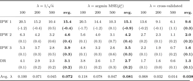
For shrinkage in combination with trimming, we also explicitly look at the nonlinear, heteroscedastic, heterogeneous design described before. We focus on the comparison of shrinkage combined with trimming rule 2 and the conventional propensity score combined with trimming rule 2. The results are given in Table 10.

Table 10: Trimmed shrinkage ATE estimators: % MSE reductions for the nonlinear, heteroscedastic, heterogeneous design

λ = 1/ √

n λ = argmin MSE(ˆ p

) λ = cross-validated

100 200 500 avg. 100 200 500 avg. 100 200 500 avg.

IPW 1 20.5 15.2 10.4 15.4 20.5 14.4 10.3 15.1 13.6 9.1 6.1 9.6

(-1.2) (-0.4) (0.5) (-0.4) (-1.7) (-1.2) (0.1) (-0.9) (-0.2) (-0.1) (1.1) (0.3)

IPW 2 6.3 4.2 3.2 4.6 5.6 4.0 3.1 4.2 2.7 2.3 1.1 2.0

(0.1) (0.4) (0.6) (0.4) (0.1) (0.3) (0.7) (0.4) (0.2) (0.1) (0.2) (0.2)

IPW 3 5.3 3.7 2.8 3.9 4.8 3.2 2.6 3.5 2.2 1.9 0.7 1.6

(0.1) (0.3) (0.5) (0.3) (0.1) (0.3) (0.6) (0.3) (0.1) (0.1) (0.2) (0.1)

DR 4.1 2.9 2.3 3.1 3.8 2.6 1.7 2.7 1.7 1.6 0.6 1.3

(0.1) (0.2) (0.2) (0.2) (0.1) (0.2) (0.3) (0.2) (0.1) (0.0) (0.1) (0.1) Avg. λ 0.100 0.071 0.045 0.072 0.118 0.078 0.047 0.081 0.068 0.032 0.014 0.038

Note:The MSE improvements due to the shrunken propensity score combined with trimming rule 2 with respect to the conventional propensity score combined with trimming rule 2 for the given method and sample size are reported along with the percentage change which is due to the bias introduced by shrinkage, i.e.,

bias2 (ATE( ˆp))−bias2 (ATE( ˆps)) bias2 (ATE( ˆp))+Var(ATE( ˆp))

, (in parentheses). ‘Avg.’ in the last columns for each method refers to the average improvement over all sample sizes. Simulation for the specification withγ= 1, ψ= 2,η=−0.3,κ= 0.8 andm2(q).

Table 10 shows that again the cross-validated λ leads to the smallest improvements when this specific setting is considered. Comparing the results based on the fixed valued λ to those based on the MSE(ˆ p ^s _i ) minimizing λ, we again find that the im- provements are very similar. Moreover, for this specific DGP, the MSE of the ATE is reduced not only due to a variance reduction, but also due to a lower squared bias, with the exception of IPW1 for n = 100 and n = 200. As for the average results, we also see that the MSE improvements for the ATE are largest for small samples, and that the improvements diminish with increasing sample size.

The detailed results for all the other DGPs are given in Tables A.4-A.15 in the Web

Appendix. The first four tables compare SH+TR2 with four competitors for the

fixed tuning parameter (A.4-A.7). Among those results, the largest improvements

are obtained for PS+TR3 in the setting with a nonlinear functional form and more controls than treated observations (see Table A.7). Here the improvements are up to 91.5% for the IPW2 estimator. If shrunken propensity scores are used with trimming rule 2 (SH+TR2) instead of the conventional propensity score (PS), the IPW1 and IPW2 estimators of ATE have up to 75.7% and 37.3% smaller MSE, respectively (Table A.4). The MSE improvements decrease slightly if SH+TR2 is used instead of PS+TR1 or PS+TR2, but they still remain considerably high.

In all 72 settings, the estimators using SH+TR2 based on the fixed tuning parameter method always outperform the estimators using PS or PS+TR1 (see Tables A.4 and A.5). In only 2 of 288 cases, the MSE of the estimator based on PS+TR2 is smaller than our suggested procedure. Furthermore, the detailed results in Table A.6 show that the losses in MSE in those two cases are only 0.1% and 0.5%. Although the estimators based on the PS+TR3 yield a lower MSE than our procedure in 12% of all cases, i.e., we observe negative improvements, the average MSE improvements across sample sizes are still high and positive (see Table A.7). Furthermore, the average of the MSE losses is only about 5%. It should be also noted that our procedure leads to higher bias reductions when compared to PS+TR3.

For the other two λ choices the overall picture is quite similar. The detailed results for the MSE(ˆ p i s)-minimizing λ in Tables A.8-A.11 show that the highest improve- ments are also observed when SH+TR2 is compared to PS+TR3. IPW1 is improved by up to 89.7%, IPW2 up to 91.5%, IPW3 up to 91.4%. For DR, the largest de- crease in MSE is 60%. In 1100 of the 1152 cases (72 settings for four estimators compared to four alternatives), our procedure yields an improvement of the MSE.

In the other 52 cases, the average increase in MSE is only 2.5%. Tables A.12-A.15

show the results for the cross-validated λ. Here too, the highest improvements are

realized relative to PS+TR3. IPW1 is improved by up to 88.4%, IPW2 and IPW3

up to 91.0%, DR up to 57.6%. In 17 of the 288 cases, SH+TR2 fails to outperform

the estimators based on conventional propensity score estimates. Traditional esti-

mates based on the conventional propensity score combined with TR1 outperform

our shrinkage approaches in only 9 of the 288 cases. If we compare our procedure to the case of the conventional propensity score combined with TR2, we see from Table A.14 that in all of the 288 cases, our procedure yields a lower MSE. The conventional propensity score combined with trimming rule 3 provide better MSE in 56 of the 288 cases. Moreover, a failure of MSE reduction due to shrinkage is rare, and the losses that do occur are small in magnitude. In the 82 cases where our procedure is outperformed, the average MSE increase is only 6.1%.

4.4. The Case of Many Covariates

In the Monte Carlo designs considered so far, only one regressor served as a con- founder for various DGPs. To get some idea of how well our shrinkage methods perform in more realistic settings, we conduct a small Monte Carlo study with many regressors. To do so, we draw the k − dimensional vector X i in Eq. (17), where k = 16, from a multivariate normal, N (0, Σ). The variance-covariance matrix Σ is set to be equal to the sample covariance between 16 variables of the National Child Development Study (NCDS) of the UK, which has been used by Blundell et al.

(2000) and Blundell et al. (2005) to estimate returns to higher education (see Table A.16 for Σ). In order to speed up the estimations, we standardize simulated covari- ates. This is equivalent to using the empirical correlation structure to generate the data. All elements of κ are set to 0.1, whereas η takes the same values as in Table 2. Thus, the combination of κ and η leads to the approximately same expected treated-to-control ratios as before, i.e. 0.57:0.43 instead of 0.6:0.4. All the other functional form specifications and coefficient configurations are the same as for the one regressor case. However, compared to the case of one confounding variable, the resulting data are less likely to suffer from overlap problem in finite samples. This can be seen from Figure A.2, which presents smoothed histograms of the estimated propensity score for all three treated-to-control ratios. Compared to Figure A.1, where we face overlap problems, there is less density mass at the boundaries.

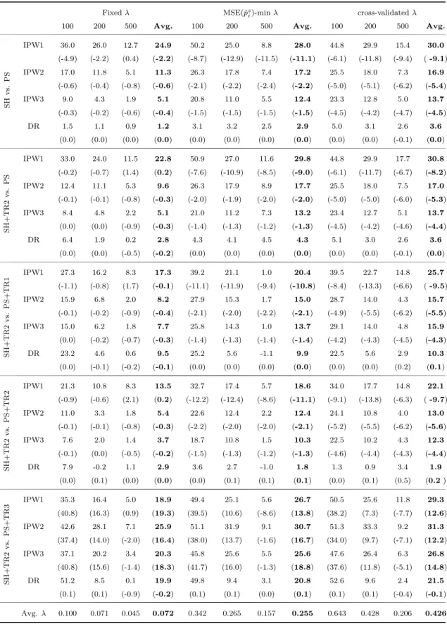
Table 11 gives the average percentage improvements across designs due to shrinkage

versus the conventional propensity score, as well as due to shrinkage in combina- tion with trimming rule 2 versus all the other methods for the fixed, the MSE(ˆ p ^s _i )- minimizing, and the cross validated λ. The first panel is equivalent to Table 5 for the multidimensional covariate vector. In contrast to the scalar X case, the cross- validated λ leads to higher improvements on average. The average improvements with fixed λ are almost always smaller than those with λs based on the other two methods.

In general, the results are quite similar to the one variable case. All λ choices lead to similar average improvements. If the benchmark is the conventional propensity score alone, or is combined either with the first or second trimming rule, the im- provements are highest for IPW1 and are increasingly lower for IPW2, IPW3, and DR, in that order. When compared to the conventional propensity score combined with trimming rule 3, the highest improvements are, in general, observed for IPW2.

All these results are consistent with the one-covariate simulation results. However,

what is very striking is that the improvements due to shrinkage either with or with-

out trimming rule 2 are very close to each other. In some cases, shrinkage alone even

outperforms the combination of shrinkage plus trimming rule 2.

Table 11: Shrinkage and trimmed shrinkage estimators: % MSE reductions, averaged across designs

Fixed

MSE(ˆ

)-min

cross-validated

100 200 500 Avg. 100 200 500 Avg. 100 200 500 Avg.

SHvs.PS

IPW1 36.0 26.0 12.7 24.9 50.2 25.0 8.8 28.0 44.8 29.9 15.4 30.0

(-4.9) (-2.2) (0.4) (-2.2) (-8.7) (-12.9) (-11.5) (-11.1) (-6.1) (-11.8) (-9.4) ( -9.1)

IPW2 17.0 11.8 5.1 11.3 26.3 17.8 7.4 17.2 25.5 18.0 7.3 16.9

(-0.6) (-0.4) (-0.8) (-0.6) (-2.1) (-2.2) (-2.4) (-2.2) (-5.0) (-5.1) (-6.2) (-5.4)

IPW3 9.0 4.3 1.9 5.1 20.8 11.0 5.5 12.4 23.3 12.8 5.0 13.7

(-0.3) (-0.2) (-0.6) (-0.4) (-1.5) (-1.5) (-1.5) (-1.5) (-4.5) (-4.2) (-4.7) (-4.5)

DR 1.5 1.1 0.9 1.2 3.1 3.2 2.5 2.9 5.0 3.1 2.6 3.6

(0.0) (0.0) (0.0) (0.0) (0.0) (0.0) (0.0) (0.0) (0.0) (0.0) (-0.1) (0.0)

SH+TR2vs.PS

IPW1 33.0 24.0 11.5 22.8 50.9 27.0 11.6 29.8 44.8 29.9 17.7 30.8

(-0.2) (-0.7) (1.4) (0.2) (-7.6) (-10.9) (-8.5) (-9.0) (-6.1) (-11.7) (-6.7) (-8.2)

IPW2 12.4 11.1 5.3 9.6 26.3 17.9 8.9 17.7 25.5 18.0 7.5 17.0

(-0.1) (-0.1) (-0.8) (-0.3) (-2.0) (-1.9) (-2.0) (-2.0) (-5.0) (-5.0) (-6.0) (-5.3)

IPW3 8.4 4.8 2.2 5.1 21.0 11.2 7.3 13.2 23.4 12.7 5.1 13.7

(0.0) (0.0) (-0.9) (-0.3) (-1.4) (-1.3) (-1.2) (-1.3) (-4.5) (-4.2) (-4.6) (-4.4)

DR 6.4 1.9 0.2 2.8 4.3 4.1 4.5 4.3 5.1 3.0 2.6 3.6

(0.0) (0.0) (-0.5) (-0.2) (0.0) (0.0) (0.0) (0.0) (0.0) (0.0) (-0.1) (0.0)

SH+TR2vs.PS+TR1

IPW1 27.3 16.2 8.3 17.3 39.2 21.1 1.0 20.4 39.5 22.7 14.8 25.7

(-1.1) (-0.8) (1.7) (-0.1) (-11.1) (-11.9) (-9.4) (-10.8) (-8.4) (-13.3) (-6.6) ( -9.5)

IPW2 15.9 6.8 2.0 8.2 27.9 15.3 1.7 15.0 28.7 14.0 4.3 15.7

(-0.1) (-0.2) (-0.9) (-0.4) (-2.1) (-2.0) (-2.2) (-2.1) (-4.9) (-5.5) (-6.2) (-5.5)

IPW3 15.0 6.2 1.8 7.7 25.8 14.3 1.0 13.7 29.1 14.0 4.8 15.9

(0.0) (-0.2) (-0.7) (-0.3) (-1.4) (-1.3) (-1.4) (-1.4) (-4.2) (-4.3) (-4.5) (-4.3)

DR 23.2 4.6 0.6 9.5 25.2 5.6 -1.1 9.9 22.5 5.6 2.9 10.3

(0.0) (-0.1) (-0.2) (-0.1) (0.0) (0.0) (0.0) (0.0) (0.0) (0.0) (0.2) (0.1)

SH+TR2vs.PS+TR2

IPW1 21.3 10.8 8.3 13.5 32.7 17.4 5.7 18.6 34.0 17.7 14.8 22.1

(-0.9) (-0.6) (2.1) (0.2) (-12.2) (-12.4) (-8.6) (-11.1) (-9.1) (-13.8) (-6.3) ( -9.7)

IPW2 11.0 3.3 1.8 5.4 22.6 12.4 2.2 12.4 24.1 10.8 4.0 13.0

(-0.1) (-0.1) (-0.8) (-0.3) (-2.2) (-2.0) (-2.0) (-2.1) (-5.2) (-5.5) (-6.2) (-5.6)

IPW3 7.6 2.0 1.4 3.7 18.7 10.8 1.5 10.3 22.5 10.2 4.3 12.3

(-0.1) (0.0) (-0.5) (-0.2) (-1.5) (-1.3) (-1.2) (-1.3) (-4.6) (-4.4) (-4.3) (-4.4)

DR 7.9 -0.2 1.1 2.9 3.6 2.7 -1.0 1.8 1.3 0.9 3.4 1.9

(0.0) (0.1) (0.0) (0.0) (0.0) (0.1) (0.1) (0.1) (0.0) (0.1) (0.5) (0.2 )

SH+TR2vs.PS+TR3

IPW1 35.3 16.4 5.0 18.9 49.4 25.1 5.6 26.7 50.5 25.6 11.8 29.3

(40.8) (16.3) (0.9) (19.3) (39.5) (10.6) (-8.6) (13.8) (38.2) (7.3) (-7.7) (12.6)

IPW2 42.6 28.1 7.1 25.9 51.1 31.9 9.1 30.7 51.3 33.3 9.2 31.3

(37.4) (14.0) (-2.0) (16.4) (38.0) (13.7) (-1.6) (16.7) (34.0) (9.7) (-7.1) (12.2)

IPW3 37.1 20.2 3.4 20.3 45.8 25.6 5.5 25.6 47.6 26.4 6.3 26.8

(40.8) (15.6) (-1.4) (18.3) (41.7) (16.0) (-1.3) (18.8) (37.6) (11.8) (-5.1) (14.8)

DR 51.2 8.5 0.1 19.9 49.8 9.4 3.1 20.8 52.6 9.6 2.4 21.5

(0.1) (0.1) (-0.9) (-0.2) (0.1) (0.1) (0.0) (0.1) (0.1) (0.1) (-0.4) (-0.1)

Avg.

0.100 0.071 0.045 0.072 0.342 0.265 0.157 0.255 0.643 0.428 0.206 0.426

Note:First panel is equivalent to Table (5) and the following panels are equivalent to Table (9) for many covariates simulation design. For further explanations see the footnotes of these tables.

The MSE improvements for the nonlinear, heteroscedastic, heterogeneous design are given in Table 12. The first part compares shrinkage to the conventional propensity score, and the second part compares shrinkage combined with trimming rule 2 to the conventional propensity score combined with trimming rule 2. The general results for this specific design with high-dimensional X are also very similar to those for the one dimensional X. One difference is that for larger sample sizes and some λ choices, shrinkage does not lead to an improvement. The DR estimator of ATE based on PS+TR2 cannot be improved by SH+TR2 even for the smallest sample size if the MSE(ˆ p ^s _i ) − minimizing or cross-validated λ is used for shrinkage.

Table 12: Shrinkage and trimmed shrinkage ATE estimators: % MSE reductions for the nonlinear, heteroscedastic, heterogeneous design (16 covariates)

λ

= 1/

= argmin MSE(ˆ

)

= cross-validated

100 200 500 avg. 100 200 500 avg. 100 200 500 avg.

SH vs. PS

IPW1 32.1 24.8 10.9 22.6 43.0 -9.7 -15.3 6.0 34.4 1.3 -21.5 4.7

(-15.9) (-7.9) (-5.3) (-9.7) (-25.8) (-44.6) (-37.8) (-36.1) (-19.6) (-43.3) (-51.7) (-38.2)

IPW2 17.2 9.4 4.1 10.3 27.2 19.2 3.9 16.8 28.3 18.1 10.0 18.8

(0.0) (0.2) (0.1) (0.1) (0.0) (0.0) (0.1) (0.0) (0.1) (0.5) (0.5) (0.3)

IPW3 9.3 3.9 2.4 5.2 22.2 9.5 3.2 11.7 27.1 14.3 8.0 16.5

(0.0) (0.1) (0.1) (0.1) (0.0) (-0.1) (0.1) (0.0) (0.1) (0.5) (0.4) (0.3)

DR 0.7 1.0 0.5 0.8 2.1 3.5 1.8 2.4 1.6 2.2 1.6 1.8

(0.0) (0.0) (-0.1) (-0.1) (0.0) (0.0) (-0.1) (0.0) (-0.1) (-0.1) (-0.5) (-0.2)

IPW1 23.0 15.3 10.7 16.4 10.0 0.6 -2.6 2.7 8.8 -6.2 -16.9 -4.8

(0.5) (0.7) (1.5) (0.9) (-38.1) (-36.8) (-22.2) (-32.4) (-30.6) (-45.3) (-40.0) (-38.6)

IPW2 8.1 4.2 -0.8 3.8 17.0 11.4 1.6 10.0 20.4 13.7 4.1 12.7

(0.1) (0.3) (-0.1) (0.1) (-0.1) (-0.1) (0.1) (0.0) (0.1) (0.5) (0.9) (0.5)

IPW3 5.8 3.4 -1.2 2.7 13.4 9.9 1.8 8.3 18.6 12.9 2.8 11.4

(0.1) (0.2) (-0.2) (0.0) (0.0) (0.0) (0.1) (0.0) (0.1) (0.5) (0.8) (0.5)

DR 5.5 0.8 -1.2 1.7 -6.5 -0.4 0.3 -2.2 -20.3 -3.3 0.5 -7.7

(0.0) (0.1) (-0.4) (-0.1) (0.0) (0.1) (-0.1) (0.0) (-0.4) (0.0) (-0.3) (-0.2)

0.100 0.071 0.045 0.072 0.345 0.269 0.159 0.257 0.646 0.426 0.210 0.427

Avg.

0.100 0.071 0.045 0.072 0.342 0.265 0.157 0.255 0.643 0.428 0.206 0.426

Note: The MSE improvements due to the shrunken propensity score combined with trimming rule 2 for the given method and sample size are reported along with the percentage change which is due to the bias introduced by shrinkage, i.e.,

bias2(ATE( ˆp))−bias2(ATE( ˆps)) bias2(ATE( ˆp))+Var(ATE( ˆp))

, (in parentheses). ‘Avg.’ in the last columns for each method refers to the average improvement over all sample sizes. Simulation for the specification withγ= 1,ψ= 2,η=−0.3,κ= 0.8 andm₂(q).

The overall picture of the case involving many covariates is not very different from that of the case involving only a single covariate. For the pairwise comparison of shrinkage vs. the conventional propensity score, in only 4 of the 288 cases is the MSE improvement negative with the fixed λ. Moreover, the increase in MSE was only 0.3% on average. If SH+TR2 is compared to all four competitors, we observe MSE improvements in, on average, 88.6% of all cases with the fixed tuning parameter.

With the MSE(ˆ p ^s _i )-minimizing and cross-validated λs, MSE is improved in 89.3%

and 90.5% of the cases, respectively.

5. Conclusion

Weighting estimators are among the most popular methods in the treatment effects literature. Despite their theoretical attractiveness these estimators suffer from large standard errors in empirical applications if the weights become too extreme due to the propensity score estimates close to the boundaries. In this paper, we propose a simple James-Stein type of shrinkage approach for the propensity score to reduce estimation risk for the average treatment effect. In order to stabilize the propen- sity score estimates we propose to shrink the conventional propensity score to the unconditional mean of the treatment variable.

We propose three different methods to choose the tuning parameter which determines the degree of shrinkage. By means of a comprehensive Monte Carlo simulation study for a wide range of simulation designs, we evaluate the finite sample properties of the shrinkage method without and with additional trimming of the propensity scores.

Our designs include simpler DGPs determined by one confounder, as well as more realistic DGPs determined by many confounders.

Shrinking the propensity score turns out to be almost certainly a meaningful strat-

egy for the designs with one confounder when compared to estimators based on

conventional propensity score estimates, as we obtain a lower MSE in all of the 288

settings if we use the fixed valued or the MSE minimizing tuning parameter. For the cross-validated tuning parameter method, in only two of the 288 designs do we find no MSE improvement, and in those cases the MSE differences between estimation without shrinkage and cross-validation based shrinkage are negligible.

Our shrinkage approach should be seen as a complementary tool to trimming as a device to cope with weights that are too large, as our shrinkage approach proves particularly appealing if it is applied jointly with trimming. In particular, we show that our procedure combined with the trimming rule proposed by Crump et al. (2009) outperforms stand-alone shrinkage and trimming approaches. The comparison of our procedure to the four competitors (estimators based on the conventional propensity score alone and combined with trimming) shows that MSE of the ATE is reduced in 96.8% of the cases with fixed λ. With the MSE(ˆ p ^s _i )-minimizing λ and the cross- validated λ, our procedure outperforms the competitors in 95.5% and 92.9% of the cases, respectively.

The findings of the simulation results with one confounder are confirmed for the more realistic case of many confounders. On average, in around 90% of the cases, for all possible pairwise comparisons and λ choices, we observe MSE improvements due to the shrinkage methods. An important difference between the one-regressor and many-regressors cases is the actual overlap between the treated and untreated subsamples. As the figures in the Appendix indicate, the former is more likely than the latter to have overlap problems in small samples. A striking finding is that shrinkage as a stand-alone method often performs best, so that additional trimming appears to be redundant.

All in all, our Monte Carlo studies show that the improvement is more pronounced if

the error term is homoscedastic. The MSE improvement of the weighting estimators

is larger when the outcome equation depends on the propensity score in a nonlinear

way. Moreover, the improvement tends to be higher when the treated-to-control

ratio is balanced. The MSE improvements are more pronounced for smaller sample

sizes, as by construction, the estimators based on the shrunken propensity score converge to the conventional estimators.

The main advantage of our approach is its simple implementation. Since the shrunken propensity scores are a simple linear combination of the conventional propensity scores and the mean of treatment variable, MSE improvements can be obtained basically without any additional computational burden. Given our different find- ings, we suggest using the shrinkage approach based on a fixed tuning parameter which vanishes with increasing sample size, as this method (as stand-alone strat- egy or combined with trimming) provides the best trade-off between MSE gain and computational burden.

Acknowledgments

The authors gratefully acknowledge financial support from the German Research

Foundation (DFG) through research unit FOR 1882 “Psychoeconomics” and from

the Oesterreichische Nationalbank (Anniversary Fund, project number: 14986). This

paper benefited from helpful ideas and discussions with Nam-Hyun Kim, Bertrand

Koebel, Fabian Kr¨uger and Bernd Fitzenberger. Furthermore, we thank the partici-

pants in the 2012 DFH Applied Econometrics Workshop in K¨onigsfeld, Germany; the

participants in the 2012 Workshop of the German Statistical Association (DStatG)

in Vienna, Austria; as well as the session participants in the 2012 European Meeting

of the Econometric Society in Malaga, Spain, for their helpful comments. We also

like to thank the editor and two anonymous referees whose comments and sugges-

tions clearly improved the paper.