Will the Sustainable Development Goals be fulfilled? Assessing present and future global poverty

Will the Sustainable Development Goals be ful fi lled? Assessing present and future global poverty

Jesús Crespo Cuaresma ^1,2,3,4 , Wolfgang Fengler ⁵ , Homi Kharas ^6,7 , Karim Bekhtiar ¹ , Michael Brottrager ⁸ &

Martin Hofer ^1,6

ABSTRACT Monitoring progress towards the fulfillment of the Sustainable Development Goals (SDGs) requires the assessment of potential future trends in poverty. This paper presents an econometric tool that provides a methodological framework to carry out pro- jections of poverty rates worldwide and aims at assessing absolute poverty changes at the global level under different scenarios. The model combines country-speci fi c historical esti- mates of the distribution of income, using Beta – Lorenz curves, with projections of population changes by age and education attainment level, as well as GDP projections to provide the fi rst set of internally consistent poverty projections for all countries of the world. Making use of demographic and economic projections developed in the context of the Intergovernmental Panel on Climate Change ’ s Shared Socioeconomic Pathways, we create poverty paths by country up to the year 2030. The differences implied by different global scenarios span worldwide poverty rates ranging from 4.5% (around 375 million persons) to almost 6% (over 500 million persons) by the end of our projection period. The largest differences in poverty headcount and poverty rates across scenarios appear for Sub-Saharan Africa, where the projections for the most optimistic scenario imply over 300 million individuals living in extreme poverty in 2030. The results of the comparison of poverty scenarios point towards the dif fi culty of ful fi lling the fi rst goal of the SDGs unless further development policy efforts are enacted.

DOI: 10.1057/s41599-018-0083-y OPEN

1

Department of Economics, Vienna University of Economics and Business (WU), 1020 Vienna, Austria.

International Institute of Applied System Analysis (IIASA), World Population Program, 2361 Laxenburg, Austria.

Wittgenstein Center for Demography and Global Human Capital (IIASA,VID/OEAW,WU), 1020 Vienna, Austria.

Austrian Institute of Economic Research, 1030 Vienna, Austria.

The World Bank, 1020 Vienna, Austria.

World Data Lab, 1070 Vienna, Austria.

The Brookings Institution, Washington, DC 20036, USA.

Johannes Kepler University, 4040 Linz, Austria. Correspondence and requests for materials should be addressed to J.C.C. (email: jcrespo@wu.ac.at)

1234567890():,;

Introduction

I n September 2015, 193 world leaders adopted the Sustainable Development Goals (SDGs) and called for a “data revolution”

(United Nations, 2013) to enhance accountability in measur- ing the progress towards their fulfillment. The SDGs have 17 goals of which the first is to “end poverty in all its forms every- where”. Extreme poverty is defined as living on less than $1.90 a day, measured in 2011 Purchasing Power Parity prices. Accessing new sources of data and refining information on SDG progress so that everyone can make use of it is a central element of this strategy. Monitoring trends in poverty reduction and providing tools that are able to assess the effects of policies on the likelihood of fulfilling this SDG are thus items which are particularly high in the agenda of priorities for the scientific community at the moment

We develop a methodological framework aimed at modeling and projecting poverty headcounts globally that builds upon the combination of new estimates of the worldwide distribution of income and macroeconomic projections of population by age and educational attainment level, as well as income per capita which have been recently developed in the context of climate change research (Lutz and KC, 2017, Crespo-Cuaresma, 2017). Using population and average income per capita projections, we provide country-specific measurements of SDG fulfillment based on the observed and potential progress in poverty reduction through the year 2030 under different scenarios embodied in the so-called Shared Socioeconomic Pathways (SSPs) (O’Neill, et al., 2014, Van Ruijven, et al., 2014, O’Neill, et al., 2017). Our contribution provides thus a link between econometric methods for research on poverty modeling and scenario-building exercises developed within the climate science community to provide a poverty pro- jection tool which is internally consistent with the figures and narratives employed in existing climate change scenarios. Our exercise complements and expands other related poverty pro- jection models which have been used in the past to assess the future of economic development at the global level. In particular, we combine efforts to compute projections of global poverty assuming no changes in within-country income distributions (Ravallion, 2013) with the latest generation of average income per capita projection models, which rely on observed global trends in human capital indicators. This allows us to improve on the methods employed in the recent literature (Edward and Sumner, 2014) by providing poverty projections which are compatible with the scenarios used in long-run prediction exercises in the climate change community.

An online tool based on the methodology described in this piece, the World Poverty Clock,

provides an informative and user-friendly visualization platform that allows the user to understand the progress and possible challenges to the fulfillment of the SDG target concerning the worldwide eradication of extreme poverty under the business-as-usual assumptions pro- vided by the SSP2 scenario.

Results and discussion

The analysis carried out provides information on 188 countries and territories, covering 99.7% of the world population (all countries and territories of the world with the exception of Aruba, Channel Islands, Curacao, Guadeloupe, French Guyana, French Polynesia, Guam, Martinique, Mayotte, New Caledonia, Reunion, Syria, US Virgin Islands and Western Sahara). The process of estimating and projecting poverty by country and scenario is carried out in three steps. First, we establish a baseline for the number of poor people in each country using the latest household survey available. Second, we “now-cast” the figure to the present.

Third, we project poverty forward to 2030 making use of the

corresponding scenario concerning future developments at the global level which is embodied in the set of population and GDP projections created within the SSPs (Lutz and KC, 2017; Crespo- Cuaresma, 2017).

For all countries for which distributional data on income or consumption exist, we estimate a Beta–Lorenz curve summariz- ing the distribution of income using information from the most recent survey. This yields parameter estimates that can then be used to obtain current predictions of the proportion of popula- tion living below the threshold of $1.90 per day in 2011 PPP terms. The poverty headcount estimates for the economies without distributional information are obtained using fitted values based on cross-country regressions of poverty headcount ratios on GDP per capita (see Materials and Methods). Since household surveys for different countries are available for dif- ferent points in time, we adjust the survey mean to the most recent year (usually 2014 or 2015) using the growth of household expenditure per capita taken from national accounts data (Pin- kovskiy and Sala-i Martin, 2016), and then repeat the first step of our procedure to derive the number of poor people in that year.

Finally, we combine scenarios of the future dynamics of average GDP per capita with assumptions on changes in the shape of the income distribution by country to project poverty headcounts.

A benchmark assessment of the potential challenges to the fulfillment of the poverty SDG can be obtained by keeping the income distribution fixed at the latest available time point and using existing forecasts or projections of average GDP per capita to create scenario-based economic growth paths for the coming decades. We create a benchmark scenario making use of GDP forecasts by the International Monetary Fund (IMF) up to 2022 to take into account medium-term cyclical characteristics for each country. We then complement these with long-term, structural economic growth projections by Crespo-Cuaresma, (2017) and Dellink, et al., (2017) for 2023–2030. The GDP projections in Dellink, et al., (2017) are based on a generalized version of the ENV-Growth model (Johansson, et al., 2013) and rely on long- term projections of physical capital, demographic trends, labor participation rates and unemployment scenarios, as well as human capital (measured by education), energy efficiency, international oil prices and total factor productivity. The pro- jection model in Crespo-Cuaresma, (2017), on the other hand, make use of an estimated macroeconomic production function in the spirit of the modeling framework put forward by Lutz, et al., (2008). The production function takes into account the differ- ences in productivity and technology innovation potential across groups of the population by age and educational attainment level.

Combining the production function estimates with the set of population projections by age and education provided by Lutz and KC, (2017), average GDP per capita projections can be retrieved. The contributions by Dellink, et al., (2017) and Crespo- Cuaresma, (2017) provide GDP projections for most countries of the world based on the five scenarios that correspond to different narratives of the SSPs, the framework used for integrated assessment models by the Intergovernmental Panel on Climate Change (Riahi, et al., 2017).

In addition to the baseline scenario, we also compute poverty

projections based on the other four scenarios which compose the

SSPs and which present different narratives about future global

socioeconomic developments. These scenarios differ in the

importance of challenges to mitigation and challenges to adap-

tation (i.e., vulnerability) to climate change. SSP1 is characterized

by low challenges for both climate change adaptation and miti-

gation resulting from income growth which does not rely heavily

on natural resources and technological change, coupled with low

fertility rate and high educational attainment. SSP2 corresponds

to the benchmark scenario and assumes the continuation of current global socioeconomic trends at the global level. In SSP3, low economic growth coupled with low educational attainment levels and high population growth at the global level are the main elements of the narrative, which is characterized by high miti- gation and adaptation challenges. SSP4 presents a narrative of worldwide polarization, with high income countries exhibiting relatively high growth rates of income, while developing econo- mies present low levels of education, high fertility and economic stagnation. Finally, SSP5 presents a scenario with high economic growth (and therefore low adaptation challenges) coupled with high demand for fossil energy from developing economies, thus increasing global CO

emissions.

We start by analyzing in detail the implied dynamics of global poverty in the benchmark scenario (SSP2) before turning to the comparison with the poverty projections corresponding to other SSPs. Global income dynamics in the last decades have led to systematic decreases in poverty rates worldwide, with the experience in India and China having played the most important role when it comes to the overall number of persons escaping absolute poverty (see Sala-i-Martin, 2006). The worldwide pov- erty rate has fallen from above 40% in 1981 to around 9% in 2017, driven by average income per capita growth in emerging markets and some developing economies. The development of within- country income inequality, on the other hand, has been very heterogeneous across countries, with increases in income inequality in India and China and decreases in many Latin American economies. The recent empirical evidence on the relationship between poverty and overall economic growth sup- ports that increases in the income level of the poor tend to be proportional to those in average income per capita (Dollar and Kraay, 2002, Dollar, et al., 2016) over the last decades. The detailed visualization of our benchmark poverty projections, including the classification of countries by SDG attainment dis- cussed below, can be found in the World Poverty Clock. It should be noted that all projections presented assume no change in the within-country distribution of income, although the modeling framework used is able to accommodate these in a straightfor- ward manner and replicate potential scenarios based on assumptions about redistribution policy.

Using the projections of the number of people living in pov- erty, we can compute the speed at which poverty is changing in each country and compare this against a counterfactual average speed that would bring poverty down to zero by the end of 2030.

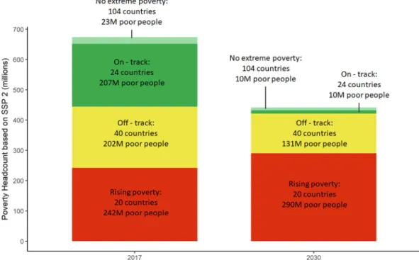
We thus compute the necessary poverty reduction speed required to fulfill the poverty SDG and use it to classify economies. If a country’s actual speed exceeds the counterfactual target, then the counterfactual target speed will fall over time. If the current speed falls short of the target, then the required target speed will rise over time to make up for the shortfall. Based on this concept, we classify economies into four groups. Some countries already have very low levels of extreme poverty. Our first grouping is of countries that have already eradicated poverty (defined by a poverty rate below 3%), termed No Extreme Poverty. A second grouping is for those countries that currently do have people living in extreme poverty, but where at projected growth, poverty will likely be eradicated before 2030. We term these as On-Track economies. A third group of countries are those which are cur- rently reducing poverty, but not at a speed which would be fast enough to achieve poverty eradication by 2030. These are clas- sified as Off-Track. A fourth group of countries are likely to see increases in the absolute numbers of people in poverty, often associated with rapid population growth. This is a group of countries with Rising Poverty. Figure 1 presents the classification for all countries in our sample for the years 2017 and 2030 in the benchmark scenario. The figure shows some countries, like India

and Indonesia, switching from On-Track to No Extreme Poverty over this time frame.

Our model estimates indicate that on September 1, 2017, 647 million people live in extreme poverty. Every minute 70 people escape poverty (or 1.2 people per second). This is close to the SDG-target (92 people per minute, or 1.5 per second) and allows us to estimate that around 36 million people have escaped extreme poverty in the year 2016. However, by 2020 the rate of poverty reduction slows down to below 50 people per minute after most of the Asian continent has already achieved the pov- erty SDG target. This implies that the big bulk of the poverty reduction challenge is expected to be in Africa, which is expected to make progress but only slowly. Today, 418 million Africans (33% of the population of the continent) live in extreme poverty.

Most countries are expected to make some progress until 2030 so that the total number of poor people would reach 373 million (23% of the population). Globally, there are 24 countries which are classified as On-Track, with 207 million poor people who are expected to leave poverty before 2030. However, the 40 Off-Track countries representing 202 million poor people will still have 131 million people living in poverty by 2030. Even worse, in 20 countries with 242 million poor people, absolute poverty will rise to 290 million (Fig. 2).

The benchmark projections of poverty by country imply a high speed of poverty reduction in South Asia, East Asia and the Pacific, fueled by the high rates of income per capita growth in India, Indonesia, Bangladesh, Philippines, China and Pakistan.

Substantial reductions in poverty in Sub-Saharan Africa are only observable from 2020 onwards. Education expansion in Ethiopia, Kenya, Mozambique, Tanzania and the Democratic Republic of Congo as embodied in the population projections in Lutz and KC, (2017), is expected to be the main factor responsible for such a development. It should be noted that the narrative of the benchmark SSP2 scenario implies worldwide income convergence trends over the present century and thus represents a relatively optimistic view of future economic development, in particular in Sub-Saharan African countries. Addressing potential changes in poverty in the context of more pessimistic scenarios appears thus as a necessary complementary exercise to address the future of worldwide poverty dynamics and understand the risks associated to the fulfillment of the SDGs.

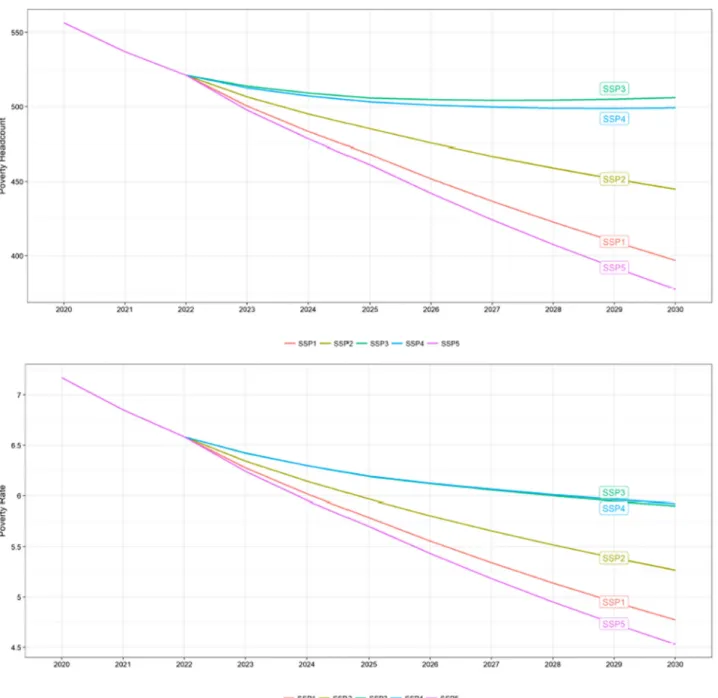
Changes in global poverty for the period 2023–2030 differ

strongly across scenarios based on the different SSPs (Fig. 3), with

the projection for SSP5 leading to approximately 377 million

persons living in extreme poverty by 2030 and that of SSP3

reaching more than 506 million (see Table 1). The largest dif-

ferences in poverty figures across scenarios tend to be con-

centrated in Sub-Saharan African countries. As compared to our

benchmark SSP2 scenario, by 2030 the number of persons living

in poverty in Nigeria implied by SSP3 would be higher by 15

million and the poverty rate would be almost 4.5 percentage

points larger. In addition to Nigeria, the Democratic Republic of

Congo, Tanzania, Uganda and Burkina Faso present the largest

differences in the absolute number of poor individuals when

comparing the benchmark poverty projections with those from

the pessimistic SSP3 scenario. Compared to the benchmark sce-

nario, the projections from the SSP3 scenario imply that four

additional countries (Bolivia, Colombia, Ethiopia and Maur-

itania) would not be able to meet the SDG goal of eradicating

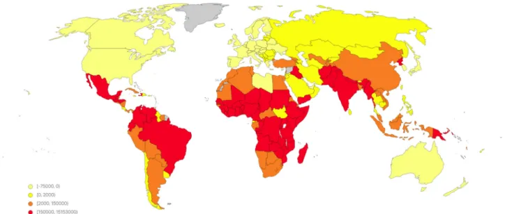
poverty by 2030. The differences in population living in extreme

poverty by country between the SSP2 (benchmark) and SSP3

(pessimistic) scenarios are presented in Fig. 4. The scenarios

imply decreases in worldwide poverty rates by almost three

percentage points in the most optimistic scenarios, around two

percentage points in the benchmark SSP2 projections and slightly

above one percentage point in the case of the pessimistic SSP3

and SSP4 scenarios. As measured by poverty rates, the absolute differences across scenarios are the largest for the African con- tinent, with the SSP5 scenario projecting a poverty rate of approximately 20% in 2030 as compared to the SSP4 projection, with implies a poverty rate of almost 26% for the same year.

The comparison of the most optimistic scenario in terms of poverty reduction (SSP5) with the benchmark projections pro- vided by the SSP2 figures reveals that the number of countries achieving poverty eradication by 2030 (as defined by having a share of extreme poor population lower than 3%) is increased only by three economies (Brazil, Burkina Faso, and Ecuador). The large reduction in poverty implied by this scenario takes place mostly in countries where poverty headcount rates are high at the moment and where high growth rates of GDP growth in the future would be able to help many persons escape poverty but would not be able to eradicate poverty in the sense implied by the

SDGs. The results of the comparison of poverty scenarios point towards the difficulty of fulfilling the first goal of the SDGs unless further development policy efforts are enacted.

In the original contributions by Dellink, et al., (2017) and Crespo-Cuaresma, (2017), the long-run average income projec- tions embodied in the SSPs are not complemented with indivi- dual within-scenario uncertainty estimates. In this respect, our poverty figures should not be considered forecasts aimed at optimizing out-of-sample predictive accuracy, but projections that provide benchmarks to understand the scope of potential poverty changes in the future under different narratives and thus inform policy makers about the possible need for policy actions and the relative progress towards fulfillment of the SDG goal. The economic growth projections provided for each SSP scenario by Crespo-Cuaresma, (2017) emphasize the role played by human capital accumulation in the form of formal education, so by

Fig. 1 Country classi fi cation by poverty eradication status: 2017, 2030

analyzing the poverty projection exercises presented we provide a first approximation to the potential (country-specific) returns of investments in education in terms of poverty reduction. The model behind the income projections in Dellink, et al., (2017) also highlights the role of trade openness as a factor affecting access to advanced technologies and thus improving productivity. By referring back to the narratives behind the different SSP scenar- ios, our projection exercise can thus inform development policy actors on how education or trade policy measures can contribute to poverty reduction in the future. The differences implied by the SSP2 and SSP1 scenarios for population by age and educational attainment described in Lutz and KC, (2017), for instance, imply different policy environments when it comes to investment in education. While SSP2 uses the so-called Global Education Trend (GET) scenario, which extrapolates the education expansion trends for developing economies using the historical experience of richer economies, SSP1 combines the GET scenario with the Fast Track (FT) scenario. The FT scenario assumes a more rapid expansion of education, mimicking the experience of South Korea, which achieved the most rapid education expansion in recent history.

Materials and methods

Projecting average income per capita by country. In order to obtain projections of average income per capita by country we combine country-specific forecasts of GDP provided by the IMF and existing income projections for SSP scenarios. The combination of short-term and medium-term GDP per capita predictions with long-term projections is carried out as follows. For observations up to the year 2022, we employ income growth forecasts sourced from the IMF’s World Eco- nomic Outlook Database. In order to ensure comparability of the projected income growth rates of GDP per capita obtained in the framework of the SSP scenarios, we use the period 2005–2015 to rebase the income growth projections by Dellink, et al., (2017) and Crespo-Cuaresma, (2017), making the average GDP per capita growth predictions in this period by these two sources be equal on average to the predictions implied by the IMF’s World Economic Outlook. For the period 2022–2030, we use the average of three income growth projections (those given by the rebased SSP projections in Dellink, et al., (2017) and Crespo-Cuaresma, (2017), as well as the average income growth implied by IMF forecasts over the period 2012–2022) to compute yearly GDP per capita figures for all countries of the world for which data are available. To compute baseline poverty projections, we use the business-as-usual projection scenario, dubbed SSP2 (Riahi, et al., 2017) from Dellink, et al., (2017) and Crespo-Cuaresma, (2017). Our method thus provides the

first set of poverty projections that are integrated with climate and demographic trends in an internally-consistent way.

The two models used to obtain long-term GDP projections employ similar narratives to define their SSP scenarios, but differ in terms of the focus on economic growth determinants. The OECD ’ s ENV-Growth model concentrates on six different drivers of income growth: Total factor productivity, physical capital, labor, energy demand and natural resource revenues. The parameters of the model linking these determinants and GDP per capita are calibrated using historical data and assumptions about the long-term equilibrium of national economies. On the other hand, the model put forward by Crespo-Cuaresma, (2017) is based on the estimation of a macroeconomic production function with heterogeneous labor input. This production function assumes that total income in the economy depends on total factor productivity, physical capital and labor input differentiated by age and educational attainment. The estimates of the elasticity of income per capita to the different production inputs are obtained using data that span the last decades and are used to project income per capita to the future.

The scenarios for GDP projections differ in terms of total factor productivity growth and capital intensity, as well as human capital dynamics, where the projections of population by age and educational attainment in Lutz and KC, (2017), which were also developed to match the SSP narratives, are used. By employing SSP-speci fi c human capital projections, the scenarios imply different labor productivity dynamics related both to education-induced skill

improvement and to shifts in the technological frontier through innovation and adoption.

The SSP1, SSP2, and SSP5 scenarios imply tendencies towards a more equal distribution of average income per capita across countries of the world, while the narratives embodied in SSP3 and SSP4 result in increases in between-country inequality. Since our poverty projections are carried out for fi xed country-speci fi c income distributions, global inequality changes in the projected period are driven by cross-country differences across scenarios.

Reconstructing the distribution of income by country. We employ aggregate survey data on quantile shares for income and consumption for the estimation of country-speci fi c poverty headcounts. Our main source is the World Bank ’ s PovCal database, which contains information on the within-country distribution of income and consumption for a large number of developing economies. For countries which are not included in the PovCal dataset, we exploit the information included in the Poverty and Equity Database (World Bank, 2017) or, if data for the particular country are not available in this source, in the UNU-WIDER’s World Income Inequality Database (UNU-WIDER, 2017).

The total coverage when combining all three datasets is of 166 countries.

Poverty headcount estimates for 22 additional economies are obtained using alternative methods described below. In order to visualize the data in the online tool of the World Poverty Clock, we use a dynamic model that provides the change in poverty per second for all countries of the world based on poverty headcount data 18 months in the past and the projected headcounts 18 months in the future.

Fig. 2 Persons living in extreme poverty by track classi fi cation (benchmark scenario), 2017, 2030

We consider the average change per second over this 3 year period with the aim of abstracting from business cycle effects and distilling low frequency changes in poverty.

For the estimation of poverty headcount ratios, we estimate country-speci fi c Beta–Lorenz curves (Datt, et al., 1998). The specification of the Beta–Lorenz curve L(p)

provides the cumulative share in total income at the cumulative population

share p as

LðpÞ

¼ p θp

ð1 pÞ

; ð1Þ where θ , γ , and δ are parameters to be estimated. Using data for both cumulative income and population shares at the quintile level, we estimate the parameters for Fig. 3 Persons living in extreme poverty and poverty rate by SSP scenario 2020 – 2030

Table 1 Poverty headcount and poverty rate by continent and SSP scenario, 2030 (millions, poverty rate in parenthesis)

Region SSP1 SSP2 SSP3 SSP4 SSP5

Africa 334.69 (21.18%) 376.42 (23.19%) 429.77 (25.68%) 427.12 (25.74%) 317.32 (20.15%)

Asia 31.72 (0.66%) 35.74 (0.73%) 40.36 (0.81%) 38.46 (0.79%) 30.62 (0.64%)

Europe 2.21 (0.30%) 2.19 (0.29%) 2.12 (0.29%) 2.16 (0.29%) 2.28 (0.30%)

North America 9.90 (1.55%) 10.70 (1.66%) 12.02 (1.89%) 11.48 (1.80%) 9.38 (1.44%)

Oceania 2.41 (5.20%) 2.66 (5.71%) 2.89 (6.39%) 2.93 (6.30%) 2.34 (4.90%)

South America 15.85 (3.43%) 17.17 (3.65%) 18.85 (3.91%) 17.01 (3.66%) 15.37 (3.34%)

World 396.78 (4.79%) 444.88 (5.29%) 506.02 (5.92%) 499.16 (5.95%) 377.29 (4.55%)

every country separately, which allow us to estimate the share of population living with an income level underneath a previously defined poverty line z. Table 2 shows the summary of point estimates for the parameters in our sample of 166 countries.

For a given mean-income μ and a given poverty line, the headcount ratio (H) can be obtained by solving

θH

ð1 HÞ

γ

H δ

ð1 HÞ

¼ 1 z

μ ð2Þ

for H. To obtain poverty headcount projections, after calibrating the Beta – Lorenz parameters to the country-specific estimated values, we replace μ in Eq. (2) with the corresponding average income per capita figure for each country and projection year, and z with the poverty threshold ($1.90 a day in 2011 Purchasing Power Parity prices). Solving Eq. (2) for the corresponding values produces poverty headcount projections for all countries for which Beta–Lorenz curves can be estimated and average GDP projections exist.

Regression-based poverty estimates. For the countries for which no income distribution data are available, we use fitted values from a poverty convergence regression model based on Ravallion, (2012). We estimate the relationship between the change in poverty and income per capita, as well as initial poverty headcount rates. The relationship follows the speci fi cation of Ravallion, (2012) closely. For each country, we use the surveys with the longest possible interval between them to calculate average annual poverty growth rates. We then estimate the model

logH

logH

ð Þ=τ ¼ β

þ β

log H

þβ

ð log y

logy

Þ=τ

þβ

logH

ð log y

logy

Þ=τ þ u

; ð3Þ

where H

is the share of absolutely poor people and y

is GDP per capita for country i. For our estimates we use PPP-adjusted GDP per capita (International Monetary Fund, 2017) instead of survey means in the regression (Pinkovskiy and Sala-i Martin, 2016). Since the countries for which we require regression-based poverty estimates are missing initial headcount figures, we estimate these (H

) using a specification linking poverty to income per capita and natural resource abundance (as captured by the dummy variable OIL

, which identi fi es oil-exporting econo- mies). We use a model estimated for a cross section of countries in 2015, the fi rst year before the SDGs started. In order to ensure that our fitted values lie between 0

and 1, we use a logit-transformed model with a speci fi cation given by

H

¼ Λ γ

þ γ

logy

þ γ

OIL

þ γ

logy

OIL

; ð4Þ

where Λ(z) ≡ e

/(1 + e

) denotes the logistic function. The parameter estimates from Eq. (4) in combination with income per capita data from our missing countries provide us with poverty rates for the year 2015 for countries for which this figure is not available. These can in turn be used as initial poverty rates in Eq.

(3) to get estimates for poverty growth and thus headcount estimates for the years 2016 to 2030. Table 3 presents the parameter estimates of the two regression models presented above.

Limitations and comparability. Our estimates for poverty are based on the parametrization of the income distribution given by the Beta–Lorenz curve. Such a specification appears reasonably robust in all countries, and therefore its use for our application lends consistency to our analysis. Different estimates of poverty may be obtained using different functional forms. For example, in World Bank, (2015), the choice between a Beta–Lorenz curve and a generalized quadratic Lorenz curve is made dependent on the fi t to the existing data. The use of a single functional form, as in our case, permits for an easier interpretation of time trends, since if different functional forms are used to estimate poverty in two survey years for the same country, it becomes hard to disentangle the impact of income changes from that of methodology for estimating poverty. Other existing poverty estimates (Milanovic and Lakner, 2013) assume a log-normal distribution for income, which Table 2 Summary statistics: Beta – Lorenz curve parameter

point estimates

γ δ θ

Mean 0.95 0.52 0.72

Std. dev. 0.04 0.07 0.13

Maximum 1.07 0.97 1.14

Minimum 0.80 0.30 0.48

Observations 166

Table 3 Regression output: Poverty equations

Logit OLS

Poverty rate (1) Log poverty rate change (2) Log of initial GDP per capita − 1.350***

(0.090)

Oil dummy 16.885* (8.905)

Log of initial GDP × Oil dummy

− 2.257** (1.070)

Log of initial poverty rate 0.002 (0.006)

GDP per capita growth − 1.933*** (0.609)

Log of initial poverty rate × GDP per capita growth

− 0.181* (0.218) Constant 9.663*** (0.725) − 0.019 (0.020)

Observations 156 129

R

0.127

Adjusted R

0.106

Note:Column (1) shows the parameter estimates of Eq. (4) based on cross-sectional data for the year 2015. Column (2) reports the estimates of the poverty convergence model as described by Eq. (3). Poverty defined by 1.9$ in 2011 PPP prices

*p< 0.1; **p< 0.05; ***p< 0.01

Fig. 4 Persons living in extreme poverty: Difference between SSP2 (benchmark) and SSP3 (pessimistic) scenarios

has clear computational advantages but is more limiting in terms of the flexibility of the shape of the distribution.

Regardless of the functional form used, it is likely that estimates become less precise for the tails of the distribution. It is for this reason that we classify countries with poverty headcount rates below 3 percent as having achieved the SDG target.

At poverty rates below this level, we are not con fi dent that our estimates of poverty are reliable. We should also note that our estimates are based on survey data, and thus suffer from the limitations of not including populations excluded from surveys. For example, we do not capture poverty among refugees, street children or the homeless, each of which could be potentially large sources of poverty. We are also not able to adjust for cost of living differences, notably between urban and rural areas, except for a handful of countries where such data is available.

Nevertheless, we believe that our poverty fi gures re fl ect the best available estimates of current levels of poverty and offer unique information on how poverty trends may unfold over the time frame of the SDGs.

Our projection exercise does not explicitly incorporate uncertainty concerning (i) the future realization of average income per capita trends, and (ii) changes in country-specific income distributions. In the context of existing GDP projections for SSP scenarios, our model combines the existing sources (which do not report uncertainty bands due to their nature as assumption-driven scenarios) into a single average income trend for each country, thus merging the dynamics implied by the interpretation of the narratives that these models entail. In order to provide comparable benchmark scenarios, the model implemented keeps within-country income distributions fixed at the present and applies these to the projected average income figures. Although some research is currently being carried out on the integration of within-country income inequality projections in the framework of SSPs (Van der Mensbrugghe, 2015), as of now no widely accepted set of projected income distributions exists. Further research in assessing the fulfillment of SDGs should incorporate these developments when they become available.

Received: 14 November 2017 Accepted: 26 February 2018

Notes

1 http://worldpoverty.io/.

References

Crespo-Cuaresma J (2017) Income projections for climate change research: a fra- mework based on human capital dynamics. Glob Environ Change 42:226–236 Datt G et al. (1998) Computational tools for poverty measurement and analysis.

International Food Policy Research Institute, Washington

Dellink R, Chateau J, Lanzi E, Magné B (2017) Long-term economic growth projections in the shared socioeconomic pathways. Glob Environ Change 42:200–214

Dollar D, Kleineberg T, Kraay A (2016) Growth still is good for the poor. Eur Econ Rev 81:68–85

Dollar D, Kraay A (2002) Growth is good for the poor. J Econ Growth 7(3):195–225 Edward P, Sumner A (2014) Estimating the scale and geography of global poverty now and in the future: How much difference do method and assumptions make? World Dev 58:67 – 82

International Monetary Fund (2017) World Economic Outlook (April 2017).

World Economic Outlook

Johansson Å, Guillemette Y, Murtin F, Turner D, Nicoletti G, de Ia Maisonneuve C, Bagnoli P, Bousquet G, Spinelle F (2013) Long-term growth scenarios, OECD Economic Department Working Papers 1000

Lutz W, Crespo-Cuaresma J, Sanderson W (2008) The demography of educational attainment and economic growth. Science 319(5866):1047

Lutz W, KC S (2017) The human core of the shared socioeconomic pathways:

Population scenarios by age, sex and level of education for all countries to 2100. Glob Environ Change 42:181–192

Milanovic B, Lakner C (2013) Global income distribution: From the fall of the berlin wall to the great recession, World Bank Policy Research Working Paper 6719 O ’ Neill BC, Kriegler E, Ebi KL, Kemp-Benedict E, Riahi K, Rothman DS, van Ruijven BJ, van Vuuren DP, Birkmann J, Kok K et al. (2017) The roads ahead: narratives for shared socioeconomic pathways describing world futures in the 21st century. Glob Environ Change 42:169–180

O’Neill BC, Kriegler E, Riahi K, Ebi KL, Hallegatte S, Carter TR, Mathur R, van Vuuren DP (2014) A new scenario framework for climate change research:

the concept of shared socioeconomic pathways. Clim Change 122(3):387–400 Pinkovskiy M, Sala-i Martin X (2016) Lights, camera...income! illuminating the

national accounts-household surveys debate. Q J Econ 131(2):579–631 Ravallion M (2012) Why don’t we see poverty convergence? Am Econ Rev 102

(1):504–523

Ravallion M (2013) How long will it take to lift one billion people out of poverty?

World Bank Res Obs 28(2):139–158

Riahi K, van Vuuren DP, Kriegler E, Edmonds J, O’Neill BC, Fujimori S, Bauer N, Calvin K, Dellink R, Fricko O, Lutz W, Popp A, Crespo-Cuaresma J, KC S, Leimbach M, Jiang L, Kram T, Rao S, Emmerling J, Ebi K, Hasegawa T, Havlik P, Humpenöder F, Silva LAD, Smith S, Stehfest E, Bosetti V, Eom J, Gernaat D, Masui T, Rogelj J, Stre fl er J, Drouet L, Krey V, Luderer G, Harmsen M, Takahashi K, Baumstark L, Doelman JC, Kainuma M, Klimont Z, Marangoni G, Lotze-Campen H, Obersteiner M, Tabeau A, Tavoni M (2017) The shared socioeconomic pathways and their energy, land use, and greenhouse gas emissions implications: an overview. Glob Environ Change 42:153–168 Sala-i Martin X (2006) The world distribution of income: falling poverty and…

convergence, period. Q J Econ 121(2):351–397

United Nations (2013) Communiqu´e, meeting of the high-level panel of eminent persons on the post-2015 development agenda in bali, indonesia, 27 March 2013, United Nations

UNU-WIDER (2017) World income inequality database (WIID3.4), World Income Inequality Database

Van der Mensbrugghe D (2015), Shared socio-economic pathways and global income distribution. In 18th Annual Conference on Global Economic Ana- lysis, pp 17–19

Van Ruijven BJ, Levy MA, Agrawal A, Biermann F, Birkmann J, Carter TR, Ebi KL, Garschagen M, Jones B, Jones R et al. (2014) Enhancing the relevance of shared socioeconomic pathways for climate change impacts, adaptation and vulnerability research. Clim Change 122(3):481–494

World Bank (2015) Development goals in an era of demographic change. The World Bank, Washington DC

World Bank (2017) Poverty and equity database. Poverty and Equity Database.

Data availability

The datasets generated during the current study are available in the Dataverse repository, https://dataverse.harvard.edu/dataset.xhtml?persistentId = doi:10.7910/DVN/XS5KQA.

The original data used to obtain the projections was sourced from the International Monetary Fund ’ s World Economic Outlook (http://www.imf.org/external/pubs/ft/weo/

2017/01/weodata/index.aspx), the World Bank ’ s World Development Indicators (http://

databank.worldbank.org/data/reports.aspx?source = world-development-indicators), the Shared Socioeconomic Pathways (https://tntcat.iiasa.ac.at/SspDb/dsd?

Action = htmlpagepage = about), the CIA ’ s World Factbook (https://www.cia.gov/library/

publications/the-world-factbook/), the World Bank ’ s PovcalNet (http://iresearch.

worldbank.org/PovcalNet/povOnDemand.aspx), the World Bank ’ s Poverty Equity Database (https://datacatalog.worldbank.org/dataset/poverty-and-equity-database) and UNU-WIDER’s World Income Inequality Database (https://www.wider.unu.edu/

download/WIID3.3).

Acknowledgements

We thank Max Roser for comments on an earlier version, as well as support by the team of the World Data Lab for the visualizations presented in worldpoverty.io, in particular Florian Scholochow (technical architecture), Maria Kolitsch (user experience), Piotr Mleczko (technical implementation), Sebastian Frank and Charmaine Taus (project coordination).

Additional information

Competing interests: The authors declare no competing fi nancial interests.

Reprints and permission information is available online at http://www.nature.com/

reprints

Publisher's note: Springer Nature remains neutral with regard to jurisdictional claims in published maps and institutional affiliations.

Open Access This article is licensed under a Creative Commons Attribution 4.0 International License, which permits use, sharing, adaptation, distribution and reproduction in any medium or format, as long as you give appropriate credit to the original author(s) and the source, provide a link to the Creative Commons license, and indicate if changes were made. The images or other third party material in this article are included in the article ’ s Creative Commons license, unless indicated otherwise in a credit line to the material. If material is not included in the article ’ s Creative Commons license and your intended use is not permitted by statutory regulation or exceeds the permitted use, you will need to obtain permission directly from the copyright holder. To view a copy of this license, visit http://creativecommons.org/

licenses/by/4.0/.

© The Author(s) 2018