THz spectroscopy in high magnetic fields

(1)

Giant directional dichroism in chiral Ni ₃ TeO ₆ in

THz spectroscopy in high magnetic fields

I N A U G U R A L - D I S S E R T A T I O N Erlangung des Doktorgrades zur

an der Mathematisch-Naturwissenschaftlichen Fakultät der Universität zu Köln

vorgelegt von

Malte Langenbach

aus Duisburg

Köln, 2019

(2)

Berichterstatter: Prof. Dr. Markus Grüninger Prof. Dr. Joachim Hemberger Vorsitzender der

Prüfungskommission: Prof. Dr. Simon Trebst

Tag der mündlichen Prüfung: 25.02.2019

(3)

The Chinese Chang‘e 4 mission which launched on December 7, 2018 has the goal to perform the first soft-landing on the far side of the moon. The landing is scheduled for January 2019, 50 years after the Apollo 11 mission landed on the opposite side of the moon. Considering the effort such a mission takes, looking at things from the other side really seems to be worth something.

In general, an effect that is different for opposite directions is called non-reciprocal. The most prominent example is that of an electrical diode where the charge transport is a non-reciprocal effect due to symmetry breaking by an inbuilt electric field. The result is that a current may flow in one direction whereas it is prevented from passing in the other direction. In optics, the term directional anisotropy refers to an effect where such a non-reciprocity holds true for all polarization states of a light beam. Such a direc- tional anisotropy can have different forms for emission, diffraction or, as in our case, absorption [1]. Different absorption for light traveling in opposite directions is called di- rectional dichroism. The general reason why such an effect can be established is founded in symmetry, or more precisely the lack thereof. This is also the reason why multiferroic materials are a good place to look for such effects [2]. A list of symmetry conditions giving rise to non-reciprocal light propagation in magnetic crystals can be found in Ref.

[1].

The multiferroic Ni

₃

TeO

₆

is an exceptional compound. The structure is both chiral and polar already at room temperature [3] so the crystal structure breaks inversion symmetry. The antiferromagnetically ordered phase below T

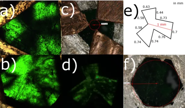
N

= 53 K features collinear spins and a significantly enhanced electric polarization due to magneto-electric coupling [4]. Despite the simple magnetic structure it exhibits non-hysteretic magnetic switch- ing and the record linear magneto-electric coupling constant in single-phase materials [4]. Those findings were made on single crystal plates of ∼1 mm×1 mm×0.1 mm [3] and

∼1 mm×1 mm×0.4 mm [4], respectively. Despite the large interest in this material in the past years, no measurements in the THz range between 100 GHz and 1000 GHz on single crystals were reported to date, simply due to the lack of single crystals large enough for measurements.

This is a general problem. New materials which are expected to exhibit exciting phys-

ical properties are often initially available as very small crystals. Crystal growth is a

time consuming process that often needs various attempts to improve a procedure which

results in large single crystals. Exemplary methods like resistivity or magnetization mea-

surements, infrared spectroscopy as well as dielectric spectroscopy in the gigahertz range

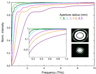
can be performed on samples of the size of a millimeter or less. However, diffraction

plays an important role in optics. When the wavelength is of the order of the sample

size, the light used for the investigation will be diffracted. In terahertz spectroscopy

the wavelengths are comparably large (1 mm at 300 GHz). Single crystals of the size of

several millimeters are usually needed. Additionally the shape of the crystal plays an

important role since preferably circular apertures are used what reduces the investigated

area of a bar-like sample drastically. The investigation of a certain material in the THz

(8)

Introduction

range starts relatively late compared to investigations in other frequency ranges where smaller samples can be measured. In our continuous wave (cw) terahertz spectrometer, we measure amplitude and phase information simultaneous. The strong influence by diffraction on the measured terahertz amplitude for small samples makes a detailed anal- ysis impossible, whereas the phase data is almost unaffected. This gives the possibility for a quantitative analysis based on the phase data, which can be supported by investi- gating relative changes in the transmittance. In this thesis, measurements on a Ni

₃

TeO

₆

sample with a surface area less than 1 mm

²

with a rather inconvenient shape due to the arrangement of domains in the crystal will be presented. We use circularly polarized light to investigate natural circular dichroism, i.e. a difference in the refractive index for the two opposite polarizations in zero magnetic field. Additionally, we will present non-reciprocal effects such as directional dichroism in an external magnetic field.

In the first part of this thesis, our setup is introduced, see Ch. 1. More details are presented on the magnetic field setup which provides an unconventional but relatively simple way of performing magnetic field dependent measurements. Furthermore, the photomixers are described due to their importance in relation to the absolute intensity, the frequency dependence of the measured phase, and the polarization of the terahertz radiation. The latter is the topic of, Ch. 2. Here, the circular polarization of the tera- hertz radiation, as well as the polarization sensitivity of the receiver to a specific circular polarization, is investigated. A method based on the polarization dependence of the re- ceiver enables to differentiate between the two opposite polarizations.

In Ch. 3, an overview of important parameters affecting the measured THz phase is given.

The influence on those parameters to the uncertainty of the phase is investigated, the main sources of errors are named, and the size of their contribution to the total error is estimated. The main contribution is caused by thermal drifts. The size of those drifts is investigated in Ch. 4, including the presentation of a method using a stable terahertz phase of a fixed terahertz frequency as reference to correct for the induced errors. The efficiency of this method is demonstrated under close-to-ideal measurement conditions as well as under extreme conditions for example for measurements in the magnetic field setup directly at low temperature and in high magnetic fields.

In Ch. 5, a discussion on chiral matter and non-reciprocal behavior is given. A general de- scription of dichroism and quadrochrosim in chiral matter based on symmetry arguments is followed by a mathematical description of the phenomena in the case of Ni

₃

TeO

₆

. Chapter 6 gives an overview on the material properties of Ni

₃

TeO

₆

based on literature.

First, the crystal structure is presented, followed by the magnetic structure. The results of recent optic spectroscopy measurements are discussed and measurements on polycrys- talline sample in the terahertz range are shown to mark the state of the research in this range. A short overview concerning the sample used for measurements during this thesis is followed by a description about dealing with problems when measuring small samples in the terahertz range, see Ch. 7.

In the last part, Ch. 8, the results for different measurements are presented. Investiga- tions with circularly polarized light in the antiferromagnetic phase show low temperature modes with a significant difference in the refractive index measured with the two helic-

2

(9)

ities. This difference in the refractive indice leads to a significant rotation of the plane

of polarization for incoming linear polarization upon passing through the sample, what

can be investigated looking at relative changes in the transmittance. Magnetic field

dependent measurements are presented for different fields up to 8 T.

(10)

(11)

1 Broadband continuous-wave THz spectrometer

In the terahertz (THz) regime, there are two different spectroscopic methods, adressing the linear response namely THz time-domain spectroscopy and THz frequency-domain spectroscopy. A variety of sources and detectors in this range as for example backward-wave oszillators, quantum-cascade lasers or free-electron lasers, black-body radiation for creating THz radiation and bolometers, Golay cells or pyroelectric detectors can be used. In THz time-domain spectroscopy, the time-dependent amplitude variation is recorded and converted into a spectrum via Fourier transformation. In THz frequency-domain spectroscopy, the amplitude and phase information is obtained for each frequency point. In our case, frequency domain spectroscopy based on the photo mixing of NIR lasers, offers a higher resolution which is only limited by the stability and width of the lasers and can reach 1 MHz [5]. For time-domain spectroscopy, the achievable spectral resolution depends on the dynamic range and is for a typical spectroscopy system ≈ 0.8 GHz at 500 GHz [6]. On the other hand the time-domain measurement offers a rela- tively high bandwidth up to 14.5 THz [7] whereas a laser based frequency domain spectra is limited by the mode-free tuning-range of the lasers which is 2.75 THz [8] up to date.

1.1 General setup

The continuous-wave (cw) THz spectrometer employed in this thesis is a setup

with components of the company Toptica. A sketch including the main compo-

nents of the cw THz spectrometer is shown in Fig. 1.1. It is an all fiber based

setup with only a small THz path in air. Responsible for creating the THz fre-

quency are the two distributed feedback (DFB) lasers [9]. The DFB lasers have

a central wavelength of 780 nm. The difference frequency, which determines the

THz frequency, is tunable from 0 THz to 1.8 THz. The frequency stability of the

DFB lasers, which is essential for the stability of the THz frequency, lies in the

MHz regime [5]. The signal of the two lasers is superimposed in a fiber array and

amplified by a tapered amplifier [10]. This amplification can be adjusted to meet

(12)

1 Broadband continuous-wave THz spectrometer

Figure 1.1: Main components of the cw THz spectrometer. The superimposed signal of two DFB lasers is amplified and split into two equal parts and guided to the two photomixers used as transmitter and receiver. Two fiber stretcher modulate the path- length to the transmitter ( L

T x

) and the receiver ( L

Rx

). Sample is placed in the optical path with length ( L

_{T Hz}

) between the two photomixers.

the power specifications of different sources and detectors. Additionally it can be adapted for example when external cooling allows for an increased laser power on the photomixers, see Sec. 1.2. The combined signal is split up into two equal parts which are guided via optical fibers to the two photomixers used as transmitter and receiver. The photomixers are described in more detail in Sec. 1.3. They determine not only the intensity of the THz radiation due to their efficiency [11], but also the polarization properties of the THz radiation, see Sec. 2, and contribute to the measured phase, see Sec. 3. The two fibers on the way to both photomixers have a length of over 60 m each due to the embedded fiber stretchers. Changing the length of the optical fibers modulates the phase which enables the extraction of the amplitude and the phase of the measured signal at each frequency [12], compare also Sec. 3.

The last part concerning the photomixers, the optical path ( L

_{T Hz}

), and the po- sition of the sample within can be varied to meet special requirements for each experiment in particular. Optical lenses can be embedded to focus the light onto the sample and/or linear polarizers can be used if necessary. An optical cryostat in the beam path can change the sample temperature from room temperature down to 3 K [13], that allows for a detailed investigation of low temperature phases. A further option is a magnetic-field setup, where the whole part including photomix- ers and sample is placed directly inside a magneto-cryostat. This is explained in more detail in Sec. 1.2. The whole electronics of the setup is placed on a mo- bile rack and can easily be moved to different labs, giving access to a variety of cryostats.

6

(13)

1.2 Design of the magnetic-field setup

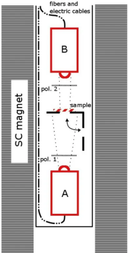
Figure 1.2: Magnetic-field setup inside the magneto-cryostat. Op- tical fibers guide the laser light to the photomixers used as transmit- ter and receiver inside the cryo- stat, directly at low temperature and in high magnetic field. Sample and reference aperture can be in- terchanged at any temperature or field using a piezo-rotator. For de- tails of the compact face-to-face as- sembly, see Fig. 1.3.

1.2 Design of the magnetic-field setup

In this setup, the antennae for creating and detecting the THz radiation are placed directly in the magneto-cryostat, at low temperatures and in high magnetic field, see Fig. 1.2. The advantage of the setup is that it overcomes the need for optical windows or focusing optics which are usually associated to the usage of an optical cryostat. Additionally, the inevitable cooling of the photomixers in this design im- proves the signal-to-noise ratio by providing the ability to increase the laser power incident on the photomixers to further increase the signal strength, and by reducing the noise in the photomixers. Furthermore, the mobile spectrometer in combina- tion with the magnetic-field setup gives access to several magneto-cryostats with different maximum magnetic-field strength and different magnetic-field configu- ration allocated at the University of Cologne. The only requirement is that the diameter of the magnet bore is large enough for the variable temperature insert (VTI) which contains the photomixers [14, 15].

To overcome the need for optical windows in the cryostat, optical fibers are trans- fered through vacuum-tight feed-troughs. About two meters of fiber lead to the two photomixers at positions P

A

and P

B

, see Fig. 1.3. The stability of the thermal gradient in the fibers plays an important role for the polarization stability of the laser light in the fibers and also for the stability of the optical path-length differ- ence, which will be discussed in Sec. 4.3.

The size is limited by the dimensions of the bore in the magnet and the space

requirements for vacuum shield and radiation shield of the VTI. The maximum

diameter of the face-to-face assembly is 34 mm; the length is 16 cm, whereas the

distance between the photomixers is around 6 cm. The antennae are equipped

(14)

1 Broadband continuous-wave THz spectrometer

with silicon lenses emitting a predominately parallel beam with a small, frequency dependent opening angle of the THz beam [16]. Therefore no additional focusing components are required. Two optional tungsten wire-grid polarizers with tita- nium frames

¹

can be embedded in the optical path when linear polarization is required, see Fig. 1.3.

An aperture mounted on a piezo-rotator allows

Figure 1.3: Compact face-to- face assembly in cryo-magnet.

Sample is placed at the cen- ter on a piezo-rotator that al- lows interchanging sample and empty reference aperture. The THz signal, created and de- tected by transmitter (P

A

) and receiver (P

B

) directly at low T and high B . Two wire grid po- larizers (pol.1 and pol.2) can be inserted if necessary.

to change sample and reference directly at any temperature or field while a temperature sensor placed on the aperture provides accurate infor- mation of the sample temperature. Since both photomixers are illuminated with nearly 30 mW laser power, the temperature directly at the pho- tomixers rises when switching on the lasers. The laser power can be increased to 100 mW using the tapered amplifier, what limits the possibil- ity of reaching the base temperature of 3 K but drastically increases the intensity of the THz ra- diation. To provide a good heat transfer to the cooling head of the VTI, almost all parts of as- sembly are made out of copper. The radiation shield prevents heating of the vacuum shield, and thereby the helium bath, by leading the radiated heat to the helium gas phase at the top of the cryostat. For a proper temperature regulation at the sample position, despite of the low thermal conductivity of the piezo-rotator, additional cop- per wires from the aperture were connected to the copper-made holder of the piezo-rotator. This al- lows a heat transport directly to the cooling-head of the VTI.

The room temperature stability of the setup was investigated previously. Details on the stability of the frequency and the phase can be found in Refs. [16, 17]. The length drift of the system was found to be up to a few tens µ m for a path-length difference of roughly 3.3 cm. This deviation is at- tributed to thermal drifts. With this magnetic-

field setup, thermal drifts are expected to play a superior role since the temperature of the fibers drops from close to 300 K over 1.3 m of fiber to 3 K. On the way to the magnetic-field setup, both fibers of the transmitter and receiver arm are placed in close proximity to ensure a minimal temperature difference between them. Close

1Build in cooperation of the mechanical workshop of the II. Institute of Physics in Cologne and the Max Planck Institute for Radioastronomy in Bonn

8

(15)

1.3 THz antennae to the photomixers, those fibers have to split up, leaving approximately 20 cm to 25 cm of length

²

especially vulnerable to temperature change. This may be caused actively by changing the temperature at the sample, changing the magnetic field leads to boiling off of some helium and a reduction of the temperature in the VTI, or simply over time by a reduction of the helium level in the surrounding cryostat.

A further discussion is given in Sec. 4.3, where also the successful reduction of this drift, using a three laser based phase correction, is presented.

1.3 THz antennae

The antennae were provided by the Max-Plank-Institute in Bonn concerning the low temperature versions. They were designed by I. Mayorga, detailed information on the principles discussed in this paragraph can be found in [11]. The log-spiral antenna structure consists of a 10/200 nm thick Ti/Au layer and was processed on the GaAs substrate using standard electron beam lithography [18]. The pho- tomixing area in the center is covered by an interdigitated finger structure of about 9×9 µm

²

. In the area covered by this structure, the illumination of the photoactive substrate with laser light leads to electron-hole excitations. The charge carriers at the photomixer used as transmitter are accelerated by an applied bias voltage and travel through the substrate to the fingers and along the spiral arms. The anten- nae radiate mainly from the so-called active region, see simulations in Ref. [19].

When the current travels along the spirals, there are regions where the current in two neighboring arms are out of phase and regions where they are in phase. The latter are the regions where radiation takes place. Detection is the inverse process to creation of THz radiation. The charge carriers in the illuminated substrate are accelerated by the THz electric field instead of an applied bias voltage, leading to a sensitivity to amplitude and phase of the measured field. Since the measured phase depends on the exact optical path which the signal has traveled, the as- sumption of the frequency-dependent active region has to be taken into account as well. A further discussion is given in Sec. 3.2 and in Sec. 7. Due to the log-spiral design, the created THz radiation can be circular over a broad range, while also the detection process at an identical photomixer is almost only sensitive to the same circular polarization. A further discussion and some spectra proving the circular character of this particular setup are presented in Sec. 2.

2Consisting of both fibers and THz path, see Eq. 3.

(16)

(17)

2 Measuring with circularly polarized light

Several recent studies show the interest of the THz community in generating and detecting broadband, circularly polarized radiation. Especially in the time do- main, huge efforts have been made recently by actively modulating the polariza- tion using four-contact photoconductive antenna [20], spiral metamaterials [21], laser-induced plasma [22], or a Fresnel rhomb [23] to create circularly polarized beams over a broad frequency range. The properties of spiral photoconductive an- tennae as transmitter were also investigated using both time-domain and cw THz spectrometers by Gregory et al. [24]. The circular polarization detection property of a spiral antenna was shown by Tsuzuki et al. [25].

2.1 Measurement principle

Historically there are two different conventions in the literature concerning the notation for right-handed circularly polarized (RCP) and left-handed circularly polarized (LCP) waves. Polarization can be defined from the point of view from the source or from the point of view at the detector. The too different conventions will result in the opposite descriptions for the same wave. We will use the first definition where RCP (LCP) corresponds to a counterclockwise (clockwise) rotation of the electic field vector when locking along the direction of energy transfer. This means positive helicity refers to a wave described by ( p− i s )/ √

2 (negative : ( p+ i s )/ √ 2 ) defined by a triplet of vectors, ( p , s , k ) which form a right-handed system.

¹

Throughout the thesis we will stick to this. Polarization states of light can be described using the Jones formalism. The electric field is

E(t) = E

0

e

^iφ^x

e

^iφ^y

1pandsstay for “parallel” and “senkrecht” as typical in optics.

(18)

2 Measuring with circularly polarized light

where E

0

is the amplitude of the field and φ

x

( φ

y

) is the phase of the x (y) component. LCP and RCP light can be described as

E

_RCP

= E

₀

√ 2 1

−i

, E

_LCP

= E

₀

√ 2 1

i

A linear polarizer P

_lin

converts circularly polarized light of one handedness into equal parts of circularly polarized light with opposite handedness and half the initial amplitude:

Figure 2.1: Left circular polarized light (green) from the source is con- verted to light with equal amounts of left- and right-handedness (grey) by a linear polarizer. The detector 2 is only sensitive to the left-handed part. Inserting a mirror directs the beam to detector 2’. Upon reflec- tion, light changes chirality. De- tector 2’ measures again only the LCP light, which interacted with the sample as RCP light

P

lin,x

E

LCP

= 1 0

0 0 E

₀

√ 2 1

i

= E

₀

√ 2 1

0 = 1 2

E

0

√ 2 1

−i

+ 1 2

E

0

√ 2 1

i

= 1

2 E

_RCP

+ 1 2 E

_LCP

Measuring samples which show, for example, significant natural optical activity needs an easy solution for measuring both circular polariza- tions independently. Even knowing photomix- ers to favor left-handedness does not immedi- ately help when the response to LCP and RCP light is expected to be different. The polariza- tion dependence of this setup was previously determined using linear polarizers and/or wave- plates [16, 26] but with older versions of the photomixers. A new method is described in Fig. 2.1. Photomixer 1, acting as source, cre- ates light with left handedness (green). Lens 1 converts the slightly diverging beam into a collinear beam which can be transformed into linearly polarized light (grey) using a linear polarizer. A second lens (2) focuses the light onto the sample

²

. Afterwards, lens 3 again cre- ates a collinear beam. Without mirror, lens 4 focuses the light on the detector 2. Now, the fact that the detector is selectively sensitive to only one chirality comes in handy, since it only

detects the left circular part of the light which passed through the sample.

To access the information contained in the right handed part, a removable mir-

2The focused beam can be guided through the windows of an optical cryostat. This is not relevant for the discussed principle, therefore it is not shown in Fig. 2.1

12

(19)

2.1 Measurement principle

Figure 2.2: Conversion of left-handed circularly polarized light, split by a linear polarizer into E

_LCP

(green) and E

_RCP

(magenta) light, into E

_RCP

’ light and E

_LCP

’ light upon reflection from at metal plate.

ror is placed in the parallel beam behind the sample. Upon reflection, a LCP (RCP) wave transform into a wave with opposite handedness (see Fig. 2.2). This means that light which passes the sample as RCP (magenta) becomes LCP (green).

Moving the focusing lens 4 and the photomixer 2 in Fig. 2.1 to positions 4’ and 2’

enables to detect amplitude and phase of this part.

A stainless steel plate as helicity converter works rather well, a rough calculation will give an idea of the conversion efficiency. The Drude contribution [27] can be used to estimate the refractive index at THz frequencies to be n ≈ 100 at 1 THz and n ≈ 200 at 300 GHz. The Brewster angle θ

_B

= arctan (n

_air

/n

_steel

) is ≈ 89.42 ° at 1 THz (and higher for lower frequencies). The calculated reflection coefficients are r

_s

= 0.986 and r

_p

= 0.972 at 1 THz. Therefor the ratio for incident circu- lar light after reflection is 0.986, leading to a slight ellipticity. The phase of r

_s

remains unchanged, whereas the phase of r

_p

is changed by exactly 180 ° so that the information contained in the left- and right-handed phase respectively remains unchanged

³

as shown in Fig. 2.2. The THz amplitude of E

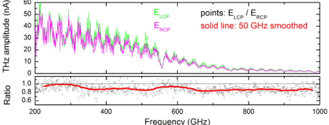
_LCP

(green in Fig. 2.3) measured at position 2 (see Fig. 2.1) with a linear polarizer between lens 1 and lens 2 reaches roughly 50 nA at 200 GHz and decreases towards 5 nA at ≈ 700 GHz.

At 1 THz, the signal is still 2 nA. Due to the long THz path in air ( ≈ 80 cm), water vapor absorption lines at 560 GHz, 750 GHz, and 988 GHz are clearly visible. The rest of the spectrum is dominated by oscillations with a period of ≈ 24 GHz caused by the booster, and a superposition of faster oscillation caused by standing waves between the different optical components. For comparison, the measured E

_RCP

is depicted as magenta line. Water absorption lines as well as the setup specific modulation of the spectrum are well reproduced. The overall amplitudes of the two polarizations are comparable at low frequencies but RPC is slightly lower be- tween 300 GHz and 550 GHz and above 650 GHz [28]. The large difference in the standing waves causes the ratio LCP/RCP to cover a broad range of 40 % (red;

Fig.2.3 lower panel). This is not surprising since by changing components in the

3This is only true for angles smaller than the Brewster angle.

(20)

2 Measuring with circularly polarized light

Figure 2.3: Top: THz amplitude of the LCP (green) and RCP (magenta) part of linear polarized light measured using the geometry described in Fig. 2.1. Bottom: Ratio of LCP to RCP THz amplitude (black, points) averaged over 50 GHz (red, solid) to overcome contributions caused by standing waves in two different THz paths.

THz path, the conditions for standing waves change completely. Smoothing the data over 50 GHz (red, solid line) diminishes the influence of the standing wave

⁴

. The signal strength for LCP and RCP is comparable over the whole frequency range and therefore an equal sensitivity for both helicities of light gives the possi- bility to explore also small differences between them.

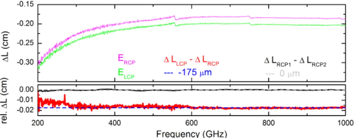
Figure 2.4 shows the path-length difference ∆L for both measurements (upper panel). Again, we see the water vapor absorption lines at 560 GHz, 750 GHz, and 988 GHz. The frequency dependence of ∆ L is explained in Sec. 3. Measuring ∆ L of RCP light (magenta) leads to a small offset due to a change in L

T Hz

. In both cases, the receiver arm is slightly longer then the transmitter arm, leading to the negative sign

⁵

. The contributions from ∆φ

_an

(ν) and ∆φ

_RC

(ν) (Sec. 3.2) have to be the same for both measurements, so subtracting ∆L

_RCP

from ∆L

_LCP

(lower panel, red line) should, in first approximation, lead to a frequency independent offset. The difference between the green and the magenta data is 175 µ m above 600 GHz. Between 300 GHz and 600 GHz, L

_{T Hz}

seems to be slightly larger (up to 15 µ m) for measuring with the mirror. Below 300 GHz the deviations rise to 70 µ m. The most probable reason is the different radius of the parallel beam for different frequencies. At 200 GHz, the full-width at half maximum (FWHM) be- hind the collimating lens is 3.5 cm. Between 200 GHz and 400 GHz this reduces drastically to 1.6 cm, whereas for higher frequencies, especially above 700 GHz, the

4Note that the exact shape of this ratio is, especially for higher frequencies, very sensitive to the overall alignment!

5This is desirable, since introducing a sample in the THz path will prolong ∆L. The phase error strongly depends on|∆L|, see Sec. 3.7.

14

(21)

2.2 Pseudo-transmittance

Figure 2.4: Top: ∆L of the left-handed (green) and right-handed (magenta) part of linear polarized light measured using the geometry described in Fig. 2.1. Bottom: Dif- ference between left- and right-handed ∆L (red, solid) and difference between two suc- cessive measurements of ∆L with right-handed light (black, circle).

FWHM stays nearly constant with a diameter of 0.8 cm [16]. A small deviation from perfect alignment of the mirror will affect the traveled path for lower fre- quencies more. Most importantly, after everything is installed, measuring ∆L

_RCP

several times leads to the same result. The difference ∆L

_RCP1

− ∆L

_RCP2

is less than 5 µ m (black, lower panel).

2.2 Pseudo-transmittance

To prove how pure the polarization state over the measured frequency range is, a rather simple experiment can be performed. Expecting the transmitter to ex- clusively radiate left-handed circularly polarized light, the light wave will, upon reflection on the mirror, be transformed into an electromagnetic wave with right handedness. Since the detector ideally should be insensitive to this, no signal can be measured. Whatever signal is still recorded is coming from one of the following scenarios:

• The transmitter emits elliptically polarized light, leading to a small right- handed part which is transformed to a left-handed wave upon reflection.

This can be detected by the detector.

• The polished metal plate does not perfectly transform the left handedness

into right handedness, leading again to a finite signal at the detector.

(22)

2 Measuring with circularly polarized light

Figure 2.5: Intensity of the non-prioritized polarization direction compared to the total intensity hitting the detector (black, dots) averaged over 50 GHz (red, solid). Spectrum shown from 100 GHz to 1300 GHz.

• The receiver is not exclusively sensitive to left-handed light. It partially records right-handed light. Thus is the same as point 1.

Comparing the recorded amplitude with and without linear polarizer directly gives a ratio which can be understood as a pseudo-transmittance of the non-prioritized polarization. The result can be seen in Fig. 2.5. The intensity E

₀²

without polarizer after reflection is reduced to 0.5 · E

₀²

with the linear polarizer, accounting for the factor of 0.5 when calculating the pseudo-transmittance. At first, the pseudo- transmittance is dominated by the shift of the standing waves induced by inserting the linear polarizer in the THz beam. It shows a spread over several percent (black dots) at low frequencies. Smoothed data increases to a maximum of ≈ 5 % at 110 GHz and ≈ 2 % at 200 GHz. Above 1.1 THz it shows a slight increase to 3 % over the next 200 GHz. Above 1.1 THz, the increase of the pseudo-transmittance is caused by the expected increasing ellipticity (see below) of the photomixers [24, 26]. Between 300 GHz and 1100 GHz, captured intensity from right handed light is less than 1 % of the intensity measured with a linear polarizer.

2.3 Discussion

The antenna geometry favors one handedness of circularly polarized light, namely LCP light. Reflecting the light from a metal plate changes the handedness of the radiation to RCP. The pseudo-transmittance shown in Fig. 2.5 gives an idea of the purity of the circular polarization because any ellipticity in the emitted THz radiation or in the sensitivity of the receiver would lead to an increased signal.

To measure the response of a sample to RCP light, a linear polarizer directly be- hind the transmitter provides equally left- and right-handed polarized light which can be guided through a sample. Now, in the reflected light, the originally RCP

16

(23)

2.3 Discussion light transforms to LCP. The polarization selective receiver measures this part independently. The results show that this comparably simple approach provides an excellent sensitivity to both circular polarizations. For higher frequencies, the area of the photomixers responsible for creating and detecting the THz radiation becomes smaller. This increases the influence of the finger structure, which is expected to develop a purely linear behavior, leading to an increasing ellipticity (compare p. 16.). The proportion of light with the other polarization state is less than 2 % from 200 GHz to 1200 GHz.

A further improvement could be made either using a gold mirror where the conduc- tivity and therefore the refractive index is larger, leading to a higher reflectivity.

Additionally, changing the setup around the cryostat enables measuring at steeper angles of ≈ 30 °. The rather large size of the collinear THz beam and therefore the need for large lenses 3 and 4’ will prevent a further decrease of this angle. Those two improvements might lead to a ratio from r

p

to r

s

of 0.997 % after reflection.

Nevertheless, the difference to the already archived ratio of 0.986 % is negligible in

the current investigation, the signal is large enough for both helicities to measure a

circular response over a broad frequency range. Important is that, if an absorption

suppresses the transmittance in RCP light to less than 1 % of the transmittance

in LCP light, the absolute strength can not be determined from the transmittance

alone, except that it might be possible to decrease the thickness of the sample.

(24)

(25)

3 Group Delay

The ability of measuring the phase directly for each frequency is one of the great advantages of cw THz spectroscopy. In chapter 8.1 we will show an example where the phase data allows the determination of sample properties even tough the amplitude is strongly influenced by diffraction. It is mandatory to investigate limitations of the accuracy of these measurements by experimental and environ- mental conditions, e.g. design of the lenses, precision or stability of the lasers, or the surroundings of the measurement setup. If all contributions are precisely determined, influences of deviations from ideal measurement conditions can be dis- cussed according to their impact on the precision of a measurement. The results discussed in this part have already been published [29].

In our setup, we extract the information of both amplitude and phase information using two fiber strechers [12]. They are positioned in the optical path where both laser frequencies are superimposed but before the two photomixers, see Sec. 1.1.

They change the optical path-length difference

∆L = L

_{T x}

+ L

_{T Hz}

− L

_Rx

(3.1)

where L

_{T x}

is the optical length of the fiber in the transmitter arm, L

_Rx

the optical length of the fiber in the receiver arm, and L

_{T Hz}

is the length of the THz path in free space. Phase data for different values of ∆L obtained in reference runs with- out any sample are shown in Fig. 3.1. At high frequencies, the dominant behavior is linear, whereas at lower frequencies a strong deviation from this linearity can be seen. In the following we will discuss all different contributions to the phase dif- ference ∆ϕ(ν) stemming from the optical fibers in both fiberarms, the transmitter and receiver photomixer, and the THz path L

_{T Hz}

, including everything between the two photomixers. A combination of all these contributions will result in a model used for fitting the data accurately in the linear and non-linear regime.

3.1 Contribution from optical fibers

The center wavelength of the lasers is around 780 nm. Depending on the desired

THz frequency, both lasers (1,2) are symmetrically detuned from the center fre-

quency ν

_1,2

= ν

₀

± ∆ν/2 where ∆ν is the terahertz frequency ν

₂

− ν

₁

. To cover

(26)

3 Group delay

Figure 3.1: Different data sets of

∆ϕ(ν) (blue) measured in face- to-face configuration. L

T Hz

( ≈ 22 cm) was changed to obtain different values of ∆L . Fre- quency step width was 1 GHz ex- cept for ∆L ≈ -0.06 mm where 100 MHz was chosen. Calculated values of ∆ϕ

_mod

(ν) (red) fitted using Eq. 3.6 with parameters

∆φ

_an

(ν

_max

) = 0.27 π and ∆L as can be seen in the plot. The com- parison between data and model yields m · 2π = 8π .

the range from 0 to 1.8 THz, the lasers wavelength has to be tuned over a range of about 2 nm each. The fibers in our setup have a light conducting core of fused silica (SiO

2

), which has a linear dispersion of about δn/δν = 4 · 10

⁻⁵

/ THz [30].

For the refractive index n

f

( ν

_1,2

) of the fiber follows

n

_f

(ν

_1,2

) =n

_f

(ν

₀

) + δn

_f

δν

ν0

· (ν

_1,2

− ν

₀

)

=n

_f

(ν

₀

) ± δn

_f

δν

ν0

· ∆ν 2

For the length L

_f

of a fiber, the phase ϕ

_f

of the optical beat is given by ϕ

_f

= L

_f

[n

_f

(ν

₂

) · ν

₂

− n

_f

(ν

₁

) · ν

₁

] · 2π

c (3.2)

With this, we find

ϕ

_f

= L

_f

n

_f

(ν

₀

) + δn

f

δν

ν0

· ν

₀

!

· 2πν

c = L

_f

· n

_{f,ef f}

· 2πν c .

The frequency-independent part in parentheses gives rise to a slight increase n

_{f,ef f}

/n

_f

≈ 1.01 , mainly because the two lasers are scanning in opposite direction from the

20

(27)

3.2 Contribution of the photomixers and antennae center frequency ν

0

. Thus, only n

f,ef f

· L

f

is relevant for the optical beat and the contribution of the optical fiber is

∆ϕ

_f

= (L

_{T x}

− L

_Rx

) · 2πν c

Here, L

_{T x}

and L

_Rx

include the effectively frequency-independent refractive index n

_{f,ef f}

of the fibers.

3.2 Contribution of the photomixers and antennae

The photomixers, each consisting of antenna, substrate, and silicon lens, deliver several contributions to the measured phase. The use of two (nearly) identical photomixers has the advantage that contributions which similarly apply to L

_Rx

and L

_{T x}

cancel out. The coupling of the optical beat into the photoactive area is identical on both sides, hence it does not contribute to ∆ϕ .

The photoconductance G depends on the terahertz frequency due to the finite carrier lifetime τ [11]. In both photomixers, this gives rise to a phase shift of ϕ

_G

= arctan(2πντ ) [24, 30]. This phase shift delays the terahertz wave in the transmitter with respect to the optical beat, which effectively increases L

_{T x}

. The phase shift in the receiver on the other hand effectively increases L

_Rx

. Therefore both contributions cancel out and do not contribute to ∆ϕ .

The total impedance of the photomixer and antenna is described by a characteris- tic time constant τ

_RC

= R

_A

C . R

_A

describes the antenna resistivity of the log-spiral antenna on the GaAs substrate [11, 31]. The contribution is nearly frequency inde- pendent, therefore R

_A

≈ 73 Ω is assumed to be constant, as the capacitance C ≈ 1.5 f F of the interdigitated electrode structure [11]. The time constant τ

_RC

≈ 0.1 ps results in a phase shift of ϕ

_RC

= arctan(2πντ

_RC

) in both, transmitter and receiver photomixer. In case of the transmitter and receiver, it contributes to L

_{T x}

. An ultra-wideband log-spiral antenna exhibits a strong dispersion and thus dis- torts short pulses [19, 32, 33, 34, 35]. The antenna effectively radiates and receives THz from the so called active region , see Sec. 1.3. A center-fed log-spiral antenna radiates where the current contributions of the two neighboring spiral arms, de- pending on the wavelength λ , interfere constructively. The radius of this active region is r

ar

=

_2π^λ

. A wave with higher wavelength has to travel a longer way l(ν) to the active region than one with lower wavelength, leading to an additional delay [35]. In time, the signal has to travel for

t

_gr,an(ν)

= l(ν) · n

_{ef f}

c (3.3)

where t

_gr,an(ν)

denotes the group delay of the antenna and n

_{ef f}

is the effective refractive index , which can be calculated to be n

_{ef f}

= p

(12.8 + 1)/2 ≈ 2.6 using

(28)

3 Group delay

the dielectric constant

GaAs

= 12.8 . The path of the spiral can be calculated to l(α(ν)) =

Z

α 0

s

r(α

⁰

)

²

+ dr

dα

⁰

dα

⁰

=

√ 1 + α

²

α (r

ar

(ν) − r

min

).

The minimum and maximum wavelength are defined by the inner and outer trun- cations respectively. With the radii r

_min

= 10 µ and r

_max

= 430 µ m and ν

_min,max

= c/2πr

_min,max

n

_{ef f}

, they are found to be ν

_max

≈ 1.8 THz and ν

_min

≈ 40 GHz, while

l(ν) = c 2πn

_{ef f}

√ 1 + α

²

α

1 ν − 1

ν

_max

. The frequency dependence of the group delay can be described as

t

_gr

= 1 2π

∂ϕ

an

∂ν

which we now integrate from ν

_max

to ν using Equ. (3.3):

Z

ν νmax

t

_gr

dν = Z

ν

νmax

√ 1 + α

²

2πα ·

1 ν − 1

ν

_max

dν = 1

2π [ϕ

_an

(ν) − ϕ

_an

(ν

_max

)]. (3.4) At each frequency, for the nearly identical photomixers as transmitter and re- ceiver, this contribution should be identical in both photomixers. Since this delay effectively prolongs the transmitter arm in both cases, the two contributions add up. This yields the final expression of the antenna characteristics for the phase difference ∆ϕ

_an

(ν) between the two arms,

∆ϕ

_an

(ν) = 2 √ 1 + α

²

α

ln ν

ν

_max

− ν ν

_max

+ 1

+ ∆ϕ

_an

(ν

_max

), (3.5) where ∆ϕ

_an

(ν

_max

) describes an offset and is treated as a fit parameter. Within the Si lenses, standing waves can cause periodic modulations of ∆ϕ(ν) [36, 37]. This effect is not important for the overall behavior of ∆ϕ(ν) , so it can be neglected for the discussion here. Nevertheless, if one considers the uncertainty of the phase as the derivative ∂∆ϕ/∂ν , this effect plays an important role, see Sec. 3.7.

3.3 Contribution of the terahertz path

The optical path length difference ∆L 3 contributes a term ∆L

^2πν_c

to ∆ϕ(ν) . This is in principle depending on the frequency ν due to water vapor in the terahertz path and standing waves between both photomixers, or photomixers and sample, but for the discussion of the overall behavior of ∆ϕ(ν) these effects deliver small contributions compared to the one of ∆ϕ

_an

(ν) . Here, it is sufficient to consider a constant value of L

_{T Hz}

. The frequency-dependent contributions nevertheless will be discussed later, see Sec. 3.7.

22

(29)

3.4 Combination of all contributions

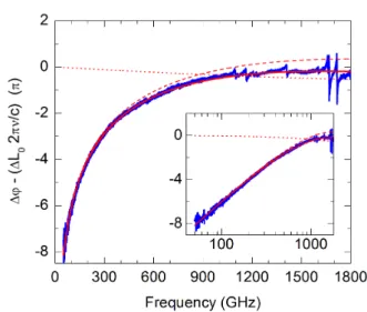
Figure 3.2: Nonlinear contribu- tions of measured phase data and model. ∆ϕ(ν) − ∆L

0

· 2πν/c for the data set with ∆L ≈ - 0.06 mm(blue) and the modeled

∆ϕ

an

(red dashed) and ∆ϕ

_RC

(red dotted). Both modeled contribu- tions add up to ∆ϕ

mod

− ∆L

0

· 2πν/c (red solid). Same data on a logarithmic frequency scale is shown in the inset

3.4 Combination of all contributions

Having determined the main contributions for ∆ϕ(ν) , we derive a model for the overall behavior taking into account the photomixer impedance (Sec. 3.2), antenna contribution (Sec. 3.2) and a constant optical path-length difference ∆L

₀

(Sec.

3.3),

∆ϕ

_mod

(ν) = ∆ϕ

_an

(ν) + ∆ϕ

_RC

(ν) + ∆L

₀

· 2πν

c . (3.6)

Using the values of the lifetime τ

_RC

= R

_A

C = 0.1 ps, the spiral growth rate a = 0.2 and ν

_max

= 1.8 THz, there remain two free parameters ∆L

₀

and the constant offset denoted by ∆ϕ

_an

(ν

_max

) , see Eq. 3.5. This simple model delivers a very accurate description of the experimental data of ∆ϕ

_an

(ν

_max

) , see Fig. 3.2. Considering an additional fit parameter γ = λ/2πr

_ar

, one finds γ = 0.997, indicating that the previous assumption for λ = 2πr

_ar

is quite accurate. ∆ϕ

_an

(ν

_max

) is then found to be 0.26 π .

The non-linear terms ∆ϕ

an

and ∆ϕ

RC

can be compared directly to the measured

∆ϕ(ν) − ∆L

₀

· 2πν/c (see Fig. 3.2). The antenna contribution clearly dominates the behavior since it changes by more than 6 π between 100 GHz and 1 THz. In the end we can define an effective, frequency-dependent optical path-length difference

∆L

_{ef f}

(ν) which is correlated to a corrected phase difference ∆ϕ

_corr

(ν) through

∆L

_{ef f}

(ν) =

_2πν^c

· ∆ϕ

_corr

(ν) . The corrected phase difference is described as the

measured phase difference ∆ϕ(ν) minus the two dominant non-linear terms ∆ϕ

_an

(30)

3 Group delay

and ∆ϕ

RC

:

∆L

_{ef f}

(ν) = c

2πν · ∆ϕ

_corr

(ν) = c

2πν · (∆ϕ(ν) − ∆ϕ

_an

− ∆ϕ

_RC

) (3.7) The result is shown in Fig. 3.3. The frequency-independent offset ∆L

₀

equals the averaged effective optical path-length difference ∆L

_{ef f}

(ν) , whereas all frequency dependence of ∆L

_{ef f}

(ν) and accordingly of ∆ϕ(ν) contains all deviations between

∆ϕ

mod

(ν) and the measured data of ∆ϕ(ν) . Without the large contributions of

∆ϕ

an

and ∆ϕ

RC

, the frequency dependence of ∆L

ef f

(ν) highlights the smaller contributions, i.e., the effective frequency dependence of ∆L

_{T Hz}

. Three main contributions can be identified.

• Standing waves within the Si lenses give rise to a modulation period of about 4.1 GHz, see inset Fig.3.3.

• Standing waves between the Si lenses separated by ∆L

T Hz

≈ 22 cm cause a modulation of 0.7 GHz.

• Resonant absorption features of water vapor.

Whereas the first two are setup specific, the resonant absorption features of water vapor, which can be seen in the main plot of Fig. 3.3, can be compared to literature [38, 39]. The absorption lines are well resolved regardless of the relatively short path in air. As a first estimate, the absorption line at 557 GHz is expected to cause a peak change of about 2 · 10

⁻⁴

of the refractive index of air [39]. For L

T Hz

≈ 22 cm, this corresponds to a change of about 40 µ m, in good agreement with our data. The two other contributions are periodic features, therefore they are better resolved in the Fourier-transformed data, see Section 3.6.

Figure 3.3: Effective optical path- length difference ∆L

_{ef f}

for the data set with ∆L

₀

≈ 0.03 mm, cf.

Eq. 3.7. Inset shows 4.07 GHz and 0.7 GHz modulation on the same data in the range of 650 GHz to 677 GHz. Modulations stem from Si lenses of the photomixers as well as standing waves in the optical path L

T Hz

between the two lenses.

Data measured with 0.1 MHz step size.

24

(31)

3.5 Active region

The design of the antennae was discussed in section 1.3. The center-fed antenna radiates mainly from the so called active region, where the currents flowing in the two spiral arms are in phase, giving rise to a constructive interference of the radiated waves [19, 40]. Following the two spiral arms r

₊

and r

−

= r

₊

· e

^aπ

, where a is the growth rate of the spiral, we consider the radius of the active region r

_ar

to be a spot with r

_ar

= (r

₊

+ r

−

)/2 which is located between the two neighboring arms. The path lengths of the two arms differ by l(r

₊

) − l(r

−

) = l(α + π) − l(α) . Since the antenna is fed in a balanced way, the currents at the minimum radius

±r

_min

are out of phase ( α = 0 ). Constructive interference occurs when the path length difference between the two arms compensates for the initial phase shift of π . The spiral radius is described as

r(α) = r

_min

e

^αa

(3.8) with r

_min

equal to the minimum radius ( ≈ 10 µ m) and a = 0.2 as the spiral growth rate. Using Eq. 3.4, one can find

λ

2 = l(α + π) − l(α) =

√ 1 + α

²

α (r

_ar

(ν) − r

_min

)(e

^aπ

− 1). (3.9) The minimum radius r

_min

is very small compared to the wavelength, therefore can be neglected for further evaluation. With this, the radius of the active region amounts to

r

_ar

= r

+

+ r

−

2 = a

4 √ 1 + a

²

e

^aπ

+ 1

e

^aπ

− 1 · λ (3.10)

using the same expression as before, γ = λ/2πr

_ar

, we find γ = 1.01 , in excel- lent agreement with our experimental results of 0.997. Theoretical studies of the radiated power density as a function of 1/ γ have been reported for different spi- ral antenna with different growth rates [41]. Here, for log-spiral antennae with a growth rate of a ≈ 0.18 ≈ 1/ tan(80

^◦

) , the power density shows a rather broad asymmetric peak at 2πr = λ/2 . It decreases only slowly towards higher values of r. In order to get a first moment, integrating from 2πr = 0.2 λ to 2 λ leads to about 0.9 λ .

3.6 Quasi-time-domain analysis

With the amplitude E

_{T Hz}

and the phase difference ∆ϕ(ν) for a discrete set of

frequency points of a certain measurement, the Fourier series as a function of the

(32)

3 Group delay

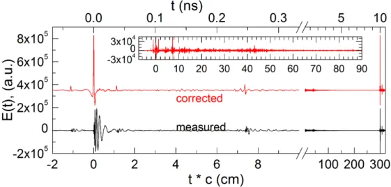
Figure 3.4: Fourier series E(t) of the data ( black ) measured up to 1.8 THz for ∆L u -0.06 mm (data from Fig. (3.3)) and after correction ( red ). Data are offset for clarity.

Scale changes at 10 cm. Measurement with frequency step width of 100 MHz yields a period of T u 300 cm. Inset shows corrected data on a different scale. Feature shifted by 7.36 cm with respect to the main peak is caused by standing waves in the Si lenses, the peak at 43.1 cm corresponds to 2 · L

_{T Hz}

and results from standing waves between the two photomixers.

time

E(t) = X

ν

E

_{T Hz}

(ν) cos(2πνt − ∆ϕ(ν)) (3.11) can be calculated. This approach is known as quasi-time-domain analysis [42].

The Fourier series is equivalent to an interferogram or to the waveform in a time- domain terahertz experiment, where all frequencies are measured simultaneously.

The main peak in the Fourier series is expected at the time t = ∆L/c . The measured data of E(t) (black line in Fig. 3.4) show a strong asymmetry around any peak. In contrast to well-defined peak positions, this is the typical shape of a strongly down-chirped signal, in which the higher frequencies arrive first. This is another visualization of the frequency dependence of the group delay introduced by the antennae. Therefore, as expected, using the corrected phase difference

∆ϕ

_corr

(ν) , see Eq. (3.7), in the Fourier series E

_corr

(t) = X

ν

E

_{T Hz}

(ν) cos(2πνt − ∆ϕ

_corr

(ν)) (3.12) removes the down-chirp and yields a pronounced "pulse" at the expected position (red line in 3.4).

26

(33)

3.7 Group delay and uncertainty of the phase The remaining peak width is caused by the limited bandwidth of the experiment and in particular the strongly decreasing amplitude with increasing frequency, see Fig. 3.4. The corrected data shows in total 5 peaks. Next to the main peak, at ± 1.1 cm (corresponding to a u 27.25 GHz modulation period), a peak occurs due to standing waves in the tapered amplifier. The amplifier is positioned before the fiber splitter, so the same modulation is later present in both fibers to the transmitter and the receiver and thus does not appear in ∆ϕ(ν) , i.e., are only observed in the amplitude. Additionally, a feature shifted by 7.36 cm (u 4.07 GHz modulation period) is visible. This reflects the periodic modulations shown in the inset of Fig. 3.3, which are caused from standing waves within the Si lenses.

The feature at 43.1 cm (u 0.7 GHz modulation period) reflects the standing waves between the two photomixers with 2 · L

_{T Hz}

u 2· 22 cm, Fig. 3.4. The feature at 86 cm is attributed to the first overtone. Using the corrected data clearly facilitates the precise determination of such features in the Fourier series.

3.7 Group delay and uncertainty of the phase

The quantitative understanding of ∆ϕ(ν) allows to further discuss the influences of experimental uncertainties determining the remaining errors of the measured phase difference. In our setup, the two experimental uncertainties contributing to the uncertainty δϕ of the measured phase difference ∆ϕ(ν) are the uncertainties of the optical path-length difference ∆L and the THz frequency ν

δϕ = ∂∆ϕ(ν)

∂ν · δν + 2πν

c · δL. (3.13)

The stability of the optical path-length difference is typically within δL =± 5 µ m, see Ch. 4. The line width of the two tunable lasers determines the line width of the beat signal, which amounts to about 5 MHz. The long term frequency stability was observed to be better than 20 MHz [5]. On the typical timescale of one sample and reference measurement which takes less than 1 h, the frequency stability is better than δν = 5 MHz. The first term of Eq. 3.13 is proportional to the group delay difference ∆t

gr

∝ ∂∆ϕ/∂ν . Starting from Eq. 3.7, we will determine the size of the errors for the different contributions.

∂∆ϕ(ν)

∂ν = ∂∆ϕ

an

∂ν + ∂ ∆ϕ

RC

∂ν + ∂ ∆L

ef f

∂ν · 2πν

c + ∆L

_{ef f}

· 2π

c (3.14)

The last term, ∆L

_{ef f}

·2π/c , dominates for large values of ∆L but can be suppressed

by choosing a small ∆L . For a larger value of ∆L = 1 cm it amounts to 0.2/ GHz.

(34)

3 Group delay

Figure 3.5: Top panel: Phase dif- ference δϕ(ν) for ∆L ≈ -0.06 mm as shown in Fig. 3.1 measured with 100 MHz as frequency step size. Middle panel: Group delay difference ∆t

_gr

compared to the contributions of the photomixer impedance (green) and the an- tenna (black). The blue curve gives a rough estimate of the envelope.

Bottom panel: same data but mul- tiplied by (c/ν)∂ν with ∂ν = 5 MHz for comparison with a change ∂L of the length.

For the data shown in Fig. 3.5 with a ∆L ≈ -60 µ m, this term can be neglected, leaving three relevant contributions.

For the fist two terms we find

∂∆ϕ

_an

∂ν = 2 √ 1 + a

²

a · ( 1 ν − 1

ν

_max

), ∂ ∆ϕ

_RC

∂ν = 4πτ

_RC

1 + (2πντ

_RC

)

²

(3.15) The comparison with the experimental data in Fig. 3.5 shows that these terms can equally be neglected. The contributions ∆ϕ

_an

and ∆ϕ

_RC

dominate the overall behavior of ∆ϕ(ν) but the derivative can be neglected when looking at

^∂∆ϕ_∂ν

. This leaves the third term

^∂∆L_∂ν^{ef f}

·

^2πν_c

, which dominates the behavior of ∂ϕ/∂ν . This is caused in particular by the contributions of the standing waves within the Si lenses and between the two photomixers. To estimate the uncertainty of the length, we roughly describe the envelope of ∂ϕ/∂ν by f(ν) = ±500/ν for ∆L ≈ -0.06 mm and L

_{T Hz}

≈ 22 cm, see bottom panel of Fig. 3.5. In order to compare the effects of frequency uncertainty versus length drift, we consider

∂ϕ · c

2πν = ∂ ∆ϕ

∂ν · c

2πν · ∂ν + ∂L (3.16)

We use the experimental result for the envelope of ±500/ν and ∂ν = 5 MHz to evaluate the first term to 0.12 µ m ·( THz /ν)

²

, which amounts to 3 µ m at 200 GHz or 0.75 µ m at 400 GHz, see middle panel of Fig. 3.5. As stated earlier, the typical length-drift observed in our setup is approximately ± 5 µ m. So for a ∂L = ± 5 µ m, and a path-length difference ∆L smaller than 1 cm, the uncertainty of the

28

(35)

3.7 Group delay and uncertainty of the phase phase for frequencies above 200 GHz is dominated by drifts of the optical path- length difference, in agreement with experimental results discussed in Ref. [5].

Knowing this, monitoring the drifts of the optical path-length difference provides

a possibility for increasing the accuracy of the phase data. A method for correcting

the drift induced changes will be described in the next chapter.

(36)

THz spectroscopy in high magnetic fields

Giant directional dichroism in chiral Ni 3 TeO 6 in