Time Preferences, Conservation and the Role of Groups: Experiments in Thailand

Time Preferences, Conservation and the Role of Groups:

Experiments in Thailand

Inauguraldissertation zur Erlangung des Doktorgrades

der Wirtschafts- und Sozialwissenschaftlichen Fakultät der Universität zu Köln

2017

vorgelegt von

Dipl.-Volksw. Suparee Boonmanunt

aus Ubon Ratchathani (Thailand)

Referent: Professor Dr. Bettina Rockenbach

Korreferent: Professor Dr. Matthias Sutter

Tag der Promotion: 13.07.2017

i The time that I spent writing this thesis has been a valuable experience and a great pleasure. Along the journey, I have benefitted from guidance and support from many people who deserve my sincere gratitude.

I am deeply grateful to Bettina Rockenbach, my supervisor and co-author, for her devoted supervision and kindness throughout these years. She has taught me not only through her lectures, writings, and valuable comments, but also through being an excellent example of an exceptional researcher and a caring supervisor.

I am also indebted to other members of the thesis committee: Oliver Gürtler and Matthias Sutter.

Many thanks to my co-authors, Thomas Lauer and Arne Weiss. Together, we have learned a lot about patience from our experiments. Working together on these projects teaches us to be patient too. Thank you so much for your patience, invaluable contribution, and a wonderful time working together.

I feel very fortunate to have a group of highly supportive friends at the office. Lea Casser, Agne Kajackaite, Uta Schier and Marcin Waligora, thank you so much for a wonderful time both inside and outside the office. I also thank my colleagues at the department of Economics, Stefania Bortolotti, Mark Pigos, Matthias Praxmarer, Anne Schielke, Sebastian Schneiders, Sebastian Tonke, Anna Untertrifaller, Christopher Zeppenfeld, Jarid Zimmerman, Nina Zimmerman and Claudia Zoller for interesting discussions and a friendly working atmosphere.

Many people have made great contribution toward my field work. My gratutide goes to Kaewsan Atibodhi, Kwansuang Atibodhi and Banjong Nasae for introducing me to people of Natithung village. I want to thank Jinda Jittanang, Charoen To-e-tae and committee members of Naithung’s Rizq Savings Group, and Sunisa Pimsen for their generous support. I thank Jintanee Jintranun for the recruitment of research and student assistants. Thank you to the students from the Department of Economics, Walailak University who provided excellent assistance in conducting the lab-in-the-field experiment. I am grateful to the villagers of Naithung for warm welcome and friendship.

For the lab experiments at Kasetsart University, Bangkok, I thank Sombat Ketrat,

Suriya Na Nongkai, Isriya Nitithanprapas, Sucheela Polruang and Decharut Sukkumnoed for

Suwannapoom and Teerawat Thammanut for the assistance in conducting the lab experiment.

My gratitude also goes to Burin Chotechaicharin, Roypimjai Jaimun, Rawadee Jarungrattanapong and Somboon Samakphan for their great assistance in both lab-in-the-field and lab experiments.

Financial support from the Economy and Environment Program for Southeast Asia (EEPSEA) for all experiments is gratefully acknowledged. I am indebted to the German Academic Exchange Service (DAAD) for granting me the full PhD scholarship.

Several friends outside academia have always supported me with their warmth and love. Chanuttha Chitpatanapaibul, Suvaporn Photjananuwat, Prae Pupityastaporn, Atit Sornsongkram, Mary Sysavanh, Patwut Tosen, Kokaew Wongpichet as well as teachers and yogi friends at Ashtanga Yoga Mitte Köln. Thank you so much.

Last but not least, I wholeheartedly thank my mother and father who care more about

my happiness than about my career. Love you.

iii

Contents

Chapter 1: Introduction ... 1

1.1 The scope of the thesis and its findings ... 2

1.2 Contribution of the thesis ... 4

Chapter 2: Time preferences and field conservation decisions: Experiment in a Thai coastal village ... 5

2.1 Introduction ... 5

2.2 The experiments ... 7

Elicitation method of time preferences ... 7

Mangrove planting as a conservation decision ... 9

2.3 Results ... 11

Measures of time preferences ... 11

Time preferences and field conservation decisions ... 12

Time preferences, membership status in savings groups and field conservation decisions ... 14

2.4 Discussion and conclusion ... 14

2.5 Appendix A: Theoretical framework of the time-preference elicitation method . ……….. 16

2.6 Appendix B: Design for time-preference elicitation ... 18

2.7 Appendix C: Implementation of payments ... 20

2.8 Appendix D: Pictures of the mangrove-planting activity ... 21

2.9 Appendix E: Regressions of absence for picking up the experiment earnings on the planting days ... 22

2.10 Appendix F: Parameter estimates of the utility functions ... 23

2.11 Appendix G: Tobit regressions for the whole sample of 180 participants ……… 25

2.12 Appendix H: Time Preferences incorporated in the standard public good model ……… 26

Chapter 3: The persuasive power of patience in groups: A lab-in-the field

experiment in rural Thailand ... 28

3.1 Introduction ... 28

3.2 Related literature ... 29

3.3 Theoretical framework and expected behaviors ... 30

3.4 The experimental design ... 32

Decisions ... 32

Treatments ... 33

Payment ... 35

Procedure ... 35

Measures of (revealed) time preferences ... 36

3.5 Results ... 37

Individual time preferences ... 37

Messages ... 38

Comparison of choices for oneself and for a group ... 39

Effects of other group members’ choices ... 41

3.6 Discussion and conclusion ... 44

3.7 Appendix A: The theoretical framework ... 46

3.8 Appendix B: Design for time-preference elicitation ... 50

3.9 Appendix C: Implementation of payments ... 52

3.10 Appendix D: Parameter estimates of the utility functions ... 53

3.11 Appendix E: The effect of others’ choices and communication on choice shifts ... ……… 56

3.12 Appendix F: Descriptive statistics of direction of choice shifts corresponding to others’ types ... 58

3.13 Appendix G: Instructions ... 60

Chapter 4: Speaking of patience: The role of others’ preferences and communication in groups ... 66

4.1 Introduction ... 66

4.2 Related literature ... 68

4.3 Theoretical framework and hypotheses ... 69

4.4 The experimental design ... 70

Decisions ... 71

v

Experimental procedure ... 73

Measures of (revealed) time preferences ... 74

4.5 Results ... 74

Choices for oneself versus for a group ... 75

Communication ... 76

Effects of others’ preferences and communication ... 77

The role of communication across subject pools ... 81

4.6 Discussion and conclusion ... 82

4.7 Appendix A: The theoretical framework ... 84

4.8 Appendix B: Design for time-preference elicitation ... 88

4.9 Appendix C: Choices and measures of time preferences in M1 and M3 treatments .. ……… 90

4.10 Appendix D: Parameter estimates of the utility functions ... 91

References ... 95

Chapter 1:

Introduction

Intertemporal decisions, which ask us, including people in rural areas in developing countrie, to trade off costs and benefits that incur at different points in time, are omnipresent.

Most of our decisions today have consequences in the future, for example, the decisions to save money, to exercise or to study, etc. We often give in the temptation to choose the option that offers the smaller but sooner benefit rather than choosing the option that offers the larger but later benefit. For instance, we end up spending all salary without saving any cents although we planned to save as we got paid. This phenomenon can be theoretically described by present-biased preferences in the quasi-hyperbolic discounting model (Laibson, 1997).

This model allows individual discount rates to decrease over time, which contradicts the assumption of constant discount rates in the discounted-utility model (e.g. Samuelson, 1937).

The summary article by Frederik, Loewenstein and O’Donoghue (2002) finds that on average individual discount rates decline over time. Individuals, however, have different discount rates across a wide range suggesting heterogeneity of individual time preferences.

In developing countries people in rural areas mostly live nearby natural resources such as fishing grounds, forest, etc. Many of them are classified as poor with regard to their financial situations. Their livelihood therefore depends tremendously on the natural resources. These people are not only the main users but can also be effective guardians of the natural resources. It is therefore important for the success of any conservation program that these local people engage in conservation activities.

A decision to conserve natural resources or not is obviously also an intertemporal

decision. For example, planting a tree requires trading-off short-run (opportunity) costs of

planting and its long-run benefits. Despite the intertemporal nature of conservation the

relationship between individual time preferences and conservation has been just recently

investigated. Previous studies still provide contradictory results. Fehr and Leibbrandt (2011)

report a negative correlation between present-biasedness and conservation among Brazillian

2 find – contrary to Fehr and Leibbrandt – that present-biasedness is unrelated to conservation among Colombian male fishermen, but more patient fishermen with lower discount rates conserve less. Their proxy for conservation behavior is a fisherman-specific fishing impact index, which takes into account fishing instruments, methods and spots.

It is therefore still crucial to study this relationship with a more direct measurement of conservation and a more detailed time-preference elicitation method. This will provide a more complete picture of how time preferences are related to conservation, which might help us to design a more effective conservation program in the field.

Furthermore, it is hard for poor households in developing countries to save regularly because both the market and the state often fail to provide access to credit and adequate protection against income or expenditure shocks (Banerjee and Duflo, 2007). It is also common among poor households that a household head is responsible for making financial decisions for the whole household, such as savings, loan taking or investments in new crops.

It will be very useful to know whether the responsibility for other people can lead to different intertemporal decisions, in particular whether it can decrease present bias.

Previous literature shows in other contexts that decisions on behalf of a group differ from decisions for oneself. Charness, Rigotti and Rustichini (2007) show in the Prisoner’s Dilemma that participants are more aggressive, i.e. strive for the largest payoff when deciding on behalf of a group than when deciding just for themselves. In addition, Sutter (2009) shows in the investment experiment that participants invest more in a lottery to have a higher probability of winning the lottery when deciding on behalf of a group than when deciding just for themselves. In other words, people try to get a higher payoff when they decide on behalf of a group than for themselves. This difference might also happen in an intertemporal context. Studying this phenomenon can give us another tool that can promote patient decisions when they are desirable.

1.1 The scope of the thesis and its findings

The thesis consists of three studies on intertemporal decisions of Thai coastal villagers

and Thai university students. The research methods are lab-in-the-field experiment, field

experiment as well as lab experiment.

Chapter 2 (Time preferences and field conservation decisions: Experiment in a Thai coastal village), joint work with Thomas Lauer, Bettina Rockenbach and Arne Weiss, ¹ investigates the relationship between time preferences and actual conservation decisions in the field. Planting mangroves is a conservation activity pursuing the long-term goal of sustaining the basis for fishing activities. The decision to engage in mangrove planting requires trading-off the short-run costs of planting with its long-run benefits. We report a lab- in-the-field experiment with Thai coastal villagers in which we elicited short- and long-run time preferences prior to a mangrove-planting activity. We show that less present-biased participants plant more mangroves, but conservation is unrelated to villagers’ long-run discounting behavior. Members of savings groups tend to plant more than non-members, suggesting a positive spill-over effect from saving decisions to other intertemporal tasks, like our conservation task.

Chapter 3 (The persuasive power of patience in groups: A lab-in-the-field experiment in rural Thailand), joint work with Thomas Lauer, Bettina Rockenbach and Arne Weiss, compares intertemporal decisions made for oneself and those made on behalf of a group. We conduct a lab-in-the-field experiment with Thai coastal villagers. First, when participants decide for themselves, their choices are on average present-biased. Then participants decide on behalf of a group of three members and prior to this decision they are informed about the choices of their group members in the individual choices. Choices for the group are significantly less present-biased than the individual choices. We show that this result is driven by an asymmetric conformity bias: learning about more patient others has a stronger influence on choices for a group than learning about less patient others.

Chapter 4 (Speaking of patience: The role of others’ preferences and communication

in groups) examines whether decisions for oneself and decisions on behalf of a group in an

intertemporal context are different among Thai university students. Participants decide first

for oneself and then decide on behalf of a group of three members. I find that choices made

for a group are significantly more patient than those made for oneself. This can be explained

by the asymmetric conformity bias toward patience through two mechanisms: other

members’ time preferences and communication between members. First, only more patient

group members are influential for decisions for a group. Second, patient messages are most

persuasive among all types of messages.

4 1.2 Contribution of the thesis

This thesis provides results and new insights that not only contribute to related existing literature but also offer possible policy implications.

Chapter 2 contributes to the recent literature by using a proxy for conservation, number of mangrove seeds planted by each participant, that can measure the concern for conservation by both female and male participants more directly than previous studies. Time preferences are also measured in a more detailed way. The negative relationship between time preferences and conservation that we find suggests that short-term (opportunity) cost can hinder local people’s conservation. A conservation program that can help people to overcome present bias might be able to enhance conservation in the field.

Chapter 3 and chapter 4 add to the literature by not just comparing intertemporal

decisions made for oneself and those made on behalf of a group. But they also explain less

present bias in decisions made on behalf of a group by the asymmetric conformity bias

toward patience. Combining all new insights of this thesis, in order to enhance field

conservation, one might consider letting representatives make conservation decisions on

behalf of a group, e.g. each household head makes decisions for her household or a head of a

savings group or a conservation group decides on conservation activities of the whole group.

Chapter 2:

Time preferences and

field conservation decisions:

Experiment in a Thai coastal village

Joint work with Thomas Lauer, Bettina Rockenbach and Arne Weiss

2.1 Introduction

Planting mangroves in tropical and subtropical tidal areas is a conservation activity that benefits the future environment (e.g., by providing nursery for aquatic animals, helping to prevent soil erosion and reducing carbon dioxide) and sustains the basis for fishing activities. ² The individual decision of the extent of engagement in mangrove planting requires trading-off short-run (opportunity) costs of planting and its long-run benefits. This intertemporal nature of conservation has stimulated research on the role of individual time preferences for conservation decisions. ³ Fehr and Leibbrandt (2011) study the relationship between present-biasedness and conservation behavior of Brazilian male fishermen. Their proxy for present-biasedness is the fishermen’s decision between a smaller amount of consumption goods now (at the beginning of their experiment) and a larger amount of the same goods two hours later (after the experiment). ⁴ The proxy for conservation is the mesh

2

For the benefits of mangroves, see Kathiresan and Bingham, 2001.

3

Conservation decisions also share a public goods character, which has been studied by e.g., Ostrom (1990), Curry,

Price and Price (2008), Burks, Carpenter, Goette and Rustichini (2009) and Poteete, Janssen and Ostrom (2010).

6 size of the fishing net or the hole size of the bottle that is used to catch shrimp. ⁵ Fehr and Leibbrandt (2011) report a negative correlation between present-biasedness and conservation:

the higher the present-biasedness the smaller the mesh or hole size. Torres-Guevara and Schlüter (2016) investigate conservation decisions of Colombian male fishermen. They measure present-biasedness similar to Fehr and Leibbrandt (2011) and additionally measure discount rates by asking fishermen to choose between a smaller amount in one week and a larger amount in two weeks. Their proxy for conservation behavior is a fisherman-specific fishing impact index, which takes into account fishing instruments, methods and spots.

Torres-Guevara and Schlüter find – contrary to Fehr and Leibbrandt – that present-biasedness is unrelated to conservation, but more patient fishermen with lower discount rates conserve less. Torres-Guevara and Schlüter explain the negative influence of patience on conservation with an indirect wealth effect: more patient fishermen have higher savings and therefore more likely invest in more efficient fishing instruments that catch more fish and thus conserve less.

We conduct a lab-in-the-field experiment with Thai fishermen which extends this research in important ways. Firstly, we extend the measurement of time-preferences. While Fehr and Leibbrandt (2011) and Torres-Guevara and Schlüter (2016) measure present- biasedness with one binary decision, we study time preferences in a more continuous way.

Like Torres-Guevara and Schlüter (2016) we also measure both present-biasedness and long- run discounting. Secondly, our experimental setup includes an independent conservation task, mangrove planting, that allows us to directly study participants’ conservation decisions. By counting the number of mangroves planted by each participant we obtain a direct measure of conservation activity, in contrast to e.g. Torres-Guevara and Schlüter’s (2016), who indirectly deduced conservation from a constructed fishing impact index. These novel aspects allow investigating how different degrees of time preferences correlate with actual conservation decisions. Moreover, we can address the inconclusive findings on the role of present- biasedness on conservation. Thirdly, in contrast to the previous studies, our subject pool includes both male and female participants.

Our lab-in-the-field experiment took place in the coastal village of Naithung, Nakhon Si Thammarat Province, Thailand. The village is located on the coastline of the Gulf of Thailand. The major economic activities are related to fisheries. We estimate the time preferences of coastal villagers based on the quasi-hyperbolic discounting model (Laibson,

5

The larger the mesh (hole) size, the easier it is for small fish (shrimp) to escape. Thus, the larger the mesh or hole

size, the higher the concern for conservation.

1997) by using the elicitation method by Andreoni and Sprenger (2012). This allows us to elicit both the long-run discounting of an individual, i.e., how an individual discounts income between two future periods, and the present-biasedness (O’Donoghue and Rabin, 1999), i.e., how an individual weights immediate income relative to income in future periods. In order to examine how elicited individual time preferences relate to conservation decisions, we organize a mangrove-planting activity on the dates participants pick up their experimental earnings. The amount of mangrove seeds a participant voluntarily plants is our proxy for her conservation decision. As this task is simple and not physically demanding, it allows us to observe the decisions of both female and male villagers of a wide range of ages.

The village hosts several savings groups that manage savings funds to help its members financially. In general, members are required to save a constant small amount of money (e.g., around USD 1.5) every month into the fund. After having been a member for some time (e.g., a year), members are eligible for micro loans as well as micro health and life insurance.

We find that less present-biased participants contribute more to the mangrove-planting activity and that planting decisions are unrelated to long-run discounting behavior. This result is robust to adding a control variable that captures membership in savings groups. Thus, our results support the findings of Fehr and Leibbrandt (2011), who also use a rather direct measurement of conservation, and stand in contrast to Torres-Guevara and Schlüter (2016), who used the indirect way of the fisherman-specific index to measure conservation.

Interestingly, members of savings groups plant weakly significantly more seeds than non-members, although membership in savings groups has no significant influence on the elicited present-biasedness and long-run discounting behavior. This suggests that membership in savings groups provides an educational effect that also spills over to our experimental conservation task. This spill-over effect underlines the importance of savings groups for sustainable development.

2.2 The experiments

Elicitation method of time preferences

We elicit time preferences through the convex time budget method (as used by

Andreoni and Sprenger, 2012; Andreoni, Kuhn and Sprenger, 2015; Lührmann, Serra-Garcia

and Winter, 2014). In this method, participants have to allocate a given budget to a sooner

and a later date at different interest rates. There are three time frames: (I) today and two

8 as time frame I and time frame III have the same time span of two weeks, but the sooner payment in time frame I is immediate. The long-run discounting parameter ( 𝛿 ) can be identified by decisions in time frame III since both payments are in the future. The experimental budget is always THB 300 (around USD 9), ⁶ which is the minimum daily wage in Thailand. The intertemporal budget constraint in each decision is therefore 𝑃𝑥 _% + 𝑥 _%'( = 300, where 𝑡 is the sooner period; 𝑘 is the time span; 𝑥 _% is the budget allocated to the sooner date; 𝑥 _%'( is the budget allocated to the later date; and 𝑃 is a gross interest rate. ⁷ There are five gross interest rates for each time frame, from 1.05 to 2.00, which corresponds to interest rates of 5% to 100% for two weeks. ⁸ These are much larger than the market interest rate at commercial banks. ⁹

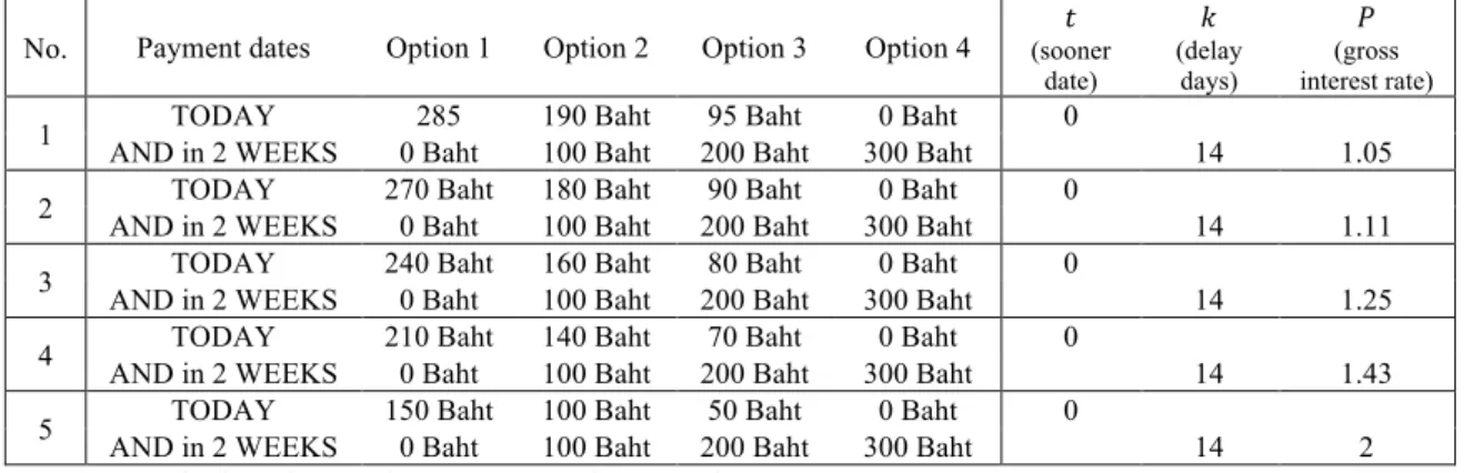
Table 2-1 summarizes all five decisions (rows in the table) for time frame I. The corresponding parameters are shown in the last three columns. The options stay the same in time frame II and time frame III, with only the timing of payments changing. For each decision, participants have to choose one favorite budget allocation out of four options.

Option 4 gives participants the highest total payoff of THB 300, but participants have to wait to get the entire amount at the later date. Option 1 gives participants the whole budget at the sooner date but discounted by the corresponding interest rate. Option 4 is therefore the most patient option, while option 1 is the least patient option. All participants have to go through all 15 decisions, which are presented one at a time.

Table 2-1: Decisions in time frame I (today,+2weeks)

No. Payment dates Option 1 Option 2 Option 3 Option 4 𝑡 (sooner

date)

𝑘 (delay

days)

𝑃 (gross interest rate)

1 TODAY 285 190 Baht 95 Baht 0 Baht 0

AND in 2 WEEKS 0 Baht 100 Baht 200 Baht 300 Baht 14 1.05

2 TODAY 270 Baht 180 Baht 90 Baht 0 Baht 0

AND in 2 WEEKS 0 Baht 100 Baht 200 Baht 300 Baht 14 1.11

3 TODAY 240 Baht 160 Baht 80 Baht 0 Baht 0

AND in 2 WEEKS 0 Baht 100 Baht 200 Baht 300 Baht 14 1.25

4 TODAY 210 Baht 140 Baht 70 Baht 0 Baht 0

AND in 2 WEEKS 0 Baht 100 Baht 200 Baht 300 Baht 14 1.43

5 TODAY 150 Baht 100 Baht 50 Baht 0 Baht 0

AND in 2 WEEKS 0 Baht 100 Baht 200 Baht 300 Baht 14 2

Note: The last three columns are not shown to the participants.

We implement a pen and paper experiment in the field. Each answer sheet is for one decision (a row in Table 2-1). Subjects see four calendars. Each calendar represents each of

6

USD 1 was equal to THB 32.62 when the experiment was conducted. THB stands for Thai Baht.

7

See the full theoretical framework in Appendix A.

8

For more details about standardized daily rate and annual rate of decisions in our experiment see Appendix B.

9

The average deposit interest rate in Thailand in 2014 is around 2.00% (The World Bank, 2016).

10

See complete decisions for all three time frames in Appendix B.

the four options. The calendars show clearly on what dates and how much money subjects will get. Subjects choose one favorite option by circling the number of their favorite calendar.

Figure 2-1 shows an example of an answer sheet for the first decision.

Figure 2-1: Example of an answer sheet

After all decisions are made, one decision is randomly drawn to determine the experimental earnings. With this mechanism, all decisions are relevant for the payoff and income effects can be avoided. The show-up fee is THB 100 (around USD 3). Participants receive an additional THB 100 for answering the post-experimental questionnaire, which is announced after the experiment. It does therefore not influence choices made in the experiment.

The issues that may turn participants reluctant to choose payoffs in the future are (1) a lack of trust that payments will be made in the future and (2) unequal transaction costs across payment dates. We address these concerns, for example, as follows: The researcher who conducted the experiment stayed in the village for two months before the experimental period. We asked the community leaders, who are trustworthy with regard to money issues, to announce the experiments for us. Furthermore, participants received a contract signed by us to guarantee their future payoffs. See Appendix C for more details about the procedure.

Mangrove planting as a conservation decision

The main objective of this study is to examine the correlation between individual time

preferences and conservation decisions. In order to observe actual conservation decisions, we

organize a mangrove-planting activity. ¹¹ We select this activity for the following reasons: (1)

mangrove planting is a simple task that everyone across genders and ages can do; (2) it takes

10 a relatively short amount of time to plant a mangrove seed; (3) another cost of planting is, however, that it is hot and dirty; (4) the villagers know about the benefits of mangroves and how to plant mangrove seeds.

The activity takes place on the days that participants come to pick up their experimental earnings. These dates depend on the random draw in each experimental session, which determines which decision will be paid out. Therefore, there are four planting days. We remind the participants through a phone call one day before their respective payment days to pick up their experimental earnings and inform them about the separate mangrove-planting activity.

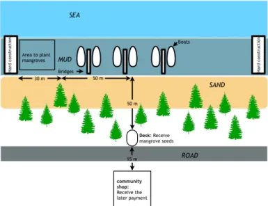
After participants pick up the experimental earnings, they are asked to go to the mangrove desk, which is located 15 meters away. Figure 2-2 illustrates the map of mangrove- planting activity. The payments are timed such that only one participant arrives at the mangrove desk at a time. Once there, participants are asked whether they would plant mangrove at all and if so, how many seeds they would like to plant. The participants receive the mangrove seeds free of charge. Willing planters then take the chosen amount of mangrove seeds to the planting area.

Figure 2-2: Map of mangrove-planting activity

To avoid that participants are influenced by reciprocity toward their experimental

earnings, we tell participants during the phone call and again at the payment desk that the

mangrove planting is a separate activity and that they should feel free not to participate. Our

data soothes any concerns about reciprocity. There is no correlation between planting

decisions and the earning from the time-preference experiment (See Table 2-2). We can also

rule out spill-overs from participants arriving earlier onto the decisions of subsequent participants. Trees block the line of sight between the mangrove desk, where participants make their planting decisions, and the mangrove-planting area. Participants can therefore not see how many mangroves have already been planted by others while they are making their own decisions.

2.3 Results

The lab-in-the-field experiment was conducted on February 21-23, 2015, in school classrooms in Naithung, Thailand. In total, 180 villagers took part in the experiment. One hundred and five participants (58%) were members of savings groups. Seventy-four participants (41%) were female. Ages ranged from 19 to 80 years old, with an average age of about 44 years. The experiment took around 80 minutes. An interview for the post- experimental questionnaire took around 30 minutes. The total average earning was THB 480.42 (around USD 16), which is about 60% higher than the minimum daily wage in Thailand.

Out of the 180 villagers who participated in the time-preference experiment, 33 (18%) did not pick up their experimental earnings. Those who were absent do not differ from participants who came to pick up their experimental earnings in terms of present-biasedness, long-run discounting and earning on the planting day. ¹² To be conservative, we only use the data of the 147 participants who came to pick up their experimental earnings and made a clear choice about their contribution to the planting activity at the site. ¹³

Measures of time preferences

We use reduced-form measures of time preferences in order to avoid making assumptions on the utility function, which would be required if we estimated parameters (see Sutter et al., 2013 for an elaboration of this argument). ¹⁴ Furthermore, this approach also allows us to have measures for all participants.

The measure of present-biasedness is calculated as the difference between the averages of the five choices made for time frame III (+2weeks,+4weeks) and for time frame I (today,+2weeks). Both time frames have the same time span of two weeks, but the sooner

12

See the regression results in Appendix E.

13

The results with all 180 participants are qualitatively similar. See Appendix G for the regression table with all 180

participants.

12 payment date is immediate in time frame I. If a participant is non-biased, then she chooses the same option in both time frames and the measure is consequently zero. ¹⁵ If a participant is present-biased, she is more patient and chooses a higher option for time frame III than for time frame I and the measure is positive. The opposite holds for a future-biased participant.

Measure of present-biasedness = Average choice in time frame III – Average choice in time frame I

For the measure of long-run discounting, we use the average of the five choices made in time frame III (scale 1 – 4), in which both payment dates are in the future so that, by definition, present-biasedness does not apply. The interpretation is along the lines of a discount factor, where higher values mean more patience, so 1 represents the least patient and 4 the most patient level.

Measure of long-run discounting = Average choice in time frame III

We observe variation in present-biasedness: 22.77% of participants are future-biased ¹⁶ , 42.86% are non-biased and 35.37% are present-biased. The participants also differ in their measure of long-run discounting, with the highest fraction (31.97%) at 0, the most patient level.

Time preferences and field conservation decisions

To answer our main research question, we now examine the relationship between experimentally elicited time preferences and our proxy for field conservation decisions, i.e., the number of mangrove seeds planted by each participant. Out of the 147 participants, 28 (19%) do not plant any seeds. The modal choice, taken by 56 participants (38%), is to plant five seeds.

We regress the number of mangrove seeds planted by each participant on the measure of present-biasedness and the measure of long-run discounting. We cluster standard errors on

15

The problem with this measure of present bias is that participants could be present-biased for some decisions and future-biased for others, leading to a bias of 0 on average. In our sample, there are few cases falling into this situation; 9 out of 63 non-biased individuals. Excluding these participants, results remain qualitatively the same. We therefore include them in the analysis.

16

Future bias is also found in previous studies, e.g. Balakrishnan, Haushofer and Jakiela (2016), Giné, Goldberg,

Silverman and Yang (2012), Takeuchi (2011).

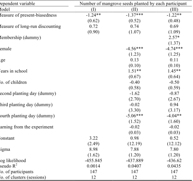
the experimental session (see Table 2-2), as proposed by Fréchette (2012). ¹⁷ We estimate Tobit models censored at zero, since 19% of participants who appeared at the activity decided not to plant. We find that present-biasedness is significantly negatively correlated with the number of mangrove seeds planted by each participant (p = 0.049 in model I). This means that more present-biased participants plant fewer mangrove seeds, which is in line with Fehr and Leibbrandt (2011). This result is robust to controlling for socio-demographic characteristics, planting day, and earnings from the time-preference experiment, ¹⁸ as shown in Table 2-2 model II (p = 0.009).

Table 2-2: Tobit regressions of the number of mangrove seeds planted by each participant Dependent variable Number of mangrove seeds planted by each participant

Model (I) (II) (III)

Measure of present-biasedness -1.24**

(0.62)

-1.37***

(0.52)

-1.22**

(0.48) Measure of long-run discounting 0.72

(0.90)

0.74 (1.07)

0.69 (1.09)

Membership (dummy) 2.57*

(1.37)

Female -4.56***

(1.23)

-4.74***

(1.25)

Age 0.13

(0.10)

0.11 (0.10)

Years in school 1.51**

(0.67)

1.45**

(0.64)

No. of children -0.40

(0.58) -0.50

(0.59)

Second planting day (dummy) -1.62

(2.70)

-0.87 (2.67)

Third planting day (dummy) -0.02

(3.30) 0.94

(3.17)

Fourth planting day (dummy) -5.06***

(1.52)

-4.04**

(1.60)

Earning from the experiment -0.02

(0.03)

-0.02 (0.03)

Constant 3.22

(2.49)

0.98 (12.19)

0.52 (12.12)

/sigma 8.98

(1.62)

7.88 (1.20)

7.80 (1.20)

Log likelihood -455.845 -437.889 -436.62

Pseudo R

0.0014 0.0407 0.0435

No. of participants 147 147 147

No. of clusters (sessions) 12 12 12

Notes: * p < 0.1, ** p < 0.05, *** p < 0.01; Robust standard errors clustered on session level in parentheses. There are 28 left-censored observations at 0 and 119 uncensored observations.

17

Although we randomly assign participants into each session and try to keep everything constant across sections,

14 The regression also shows a positive correlation between long-run discounting and the number of planted seeds, which, however, fails to be statistically significant (p = 0.42 in model I and p = 0.49 in model II). The sign of the coefficient suggests that, if there is any relationship at all, the participants who discount the future less (are more patient) tend to plant more seeds (recall that higher values of our measure of long-run discounting mean higher patience). This stands in contrast to Torres-Guevara and Schlüter (2016), who find fishermen with lower discount rates (higher long-run discounting) to harm the environment significantly more.

Result: More present-biased participants plant fewer mangrove seeds. Long-run discounting seems to be unrelated to conservation decisions.

Time preferences, membership status in savings groups and field conservation decisions

The negative correlation between the measure of present-biasedness and conservation decisions are still significant (p = 0.009) when we add membership of local savings groups as a control variable in the Tobit regression censored at zero (members: n = 95; and non- members: n = 52), as shown in Table 2-2 model (III). Controlling for membership is important because members tend to be less present-biased and less future-oriented, though not statistically significantly so (means of measure of present-biasedness is 0.12 for members vs. 0.25 for non-members, Mann-Whitney rank-sum test: p = 0.14; means of measure of long-run discounting is 2.90 for members vs. 3.04 for non-members, Mann-Whitney rank- sum test: p = 0.44). Interestingly, the model also suggests that members of savings groups plant more seeds than non-members, as the coefficient of the membership dummy is positive and weakly significant (p = 0.063).

The regression also exhibits a strong negative gender and a strong positive education effect. The strong and significant negative effect of being female might be due to a cultural effect. Thai women dislike to be exposed to the sun and try to avoid it as much as possible.

The strong positive and significant effect of education (years in school) is also remarkable.

2.4 Discussion and conclusion

In order to investigate the relationship between time preferences and field conservation

decisions, we elicit the time-preferences of Thai coastal villagers and thereafter observe their

conservation decisions in a mangrove-planting activity. Fehr and Leibbrandt (2011) find that

a less present-biased fisherman fishes in a more sustainable way, while Torres-Guevara and Schlüter (2016) find no relationship between present-biasedness and conservation, as measured by their fishing impact index, which takes instruments, methods and spots into account. Instead, they find a negative influence of patience on conservation, i.e. the more patient (lower discount rate or higher long-run discounting), the less conservation. To provide further evidence, we measure conservation more directly, i.e., by the number of mangrove seeds planted by each participant. We find a significant negative correlation between present- biasedness and field conservation, which is in line with Fehr and Leibbrandt (2011). By contrast, long-run discounting seems to be unrelated to conservation behavior. Hence, it seems that despite not eliciting long-run discounting behavior, Fehr and Leibbrandt (2011) did not leave out an additional important aspect of time preferences for conservation decisions. The results by Fehr and Leibbrandt (2011) and us suggest that more patient individuals, in terms of their present-biasedness, care more about conserving the environment. However, the results by Torres-Guevara and Schlüter (2016) warn us that this may not necessarily translate into a lower overall environmental impact if being more patient also enables fishermen to be more economically productive.

We also find that members of savings groups conserve weakly significantly more than non-members in our experimental conservation task. This result suggests a spill-over effect of savings groups on a real task that requires trading-off short-run costs and long-run benefits.

Our findings suggest that such savings groups could provide double benefits to sustainable

development: helping members to save regularly (Rutherford, 2001) and training them to

resist smaller short-run benefits in exchange for larger future benefits even in pro-social

intertemporal tasks, such as the conservation behavior studied in this chapter.

16 2.5 Appendix A: Theoretical framework of the time-preference

elicitation method

Present-biased time preference can be modeled with a simple functional form as quasi- hyperbolic discounting (Laibson, 1997).

(A2.1) where is the discount function; 𝑘 is time period; is a discount factor; and is a parameter for present-biased preference with . corresponds to the case of standard exponential discounting. The one period discount factor between the present and a future period is , while the one period discount factor between two future periods is . By including present-biased preferences into a standard intertemporal utility function, we get the following total utility function:

(A2.2) Assume a time-separable CRRA utility function ¹⁹ , in which the utility depends on the monetary payoff. In addition, there are only two time periods or dates that an agent has to allocate a given budget to (Andreoni and Sprenger, 2012; Andreoni et al., 2015). The utility function has the following form:

(A2.3) where is the amount allocated to the sooner date, while is the amount allocated to the later date. The parameter 𝛼 captures the curvature of the utility function.

Agents are assumed to maximize their total utility over time subject to the budget constraint,

(A2.4) where is the gross interest rate, is the budget.

Maximizing (3) subject to (4) gives the following conditions:

(A2.5)

where is an indicator for whether Rewriting the equation by substituting 𝑥 _%'( = 𝑌 − 𝑃𝑥 _% (from equation (4)) gives:

19

The CRRA (constant relative risk aversion) utility function:

€

D(k) = 1 βδ

⎧ ⎨

⎩ if if

k = 0 k > 0,

€

D(k)

€

δ

€

β

€

0 ≤ β < 1

€

β = 1

€

βδ

€

δ

€

U

= u(c

) + β δ

^u(c

).

k=1 T

∑

€

U(x

, x

) = x

^α + βδ

^x

α

x ^α

+ δ

^x

α

⎧ ⎨

⎩

if if

t = 0 t > 0,

€

x

€

x

€

Px

+ x

= Y ,

€

P

€

Y

x

x

= (P β

δ

)

1 α−1

,

€

t

€

t = 0.

€

U( x) = x ^α .

(A2.6) This Equation (6) tells us that the higher present bias parameter 𝛽 and/or the higher discount factor 𝛿 leads to the higher fraction of the budget which is allocated to the sooner date 𝑥 _% .

For parameter estimation, take log to equation (5):

(A2.7)

€

x

= Y (P β

δ

⁾

1

α

1 + P(P β

δ

⁾

1

α

.

€

ln x

x

⎛

⎝ ⎜ ⎞

⎠ ⎟ = ln( β ⁾

α − 1 t

+ ln( δ ⁾

α − 1 k + 1

α − 1 ln(P).

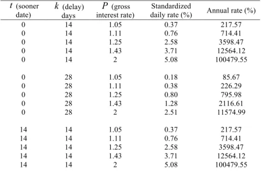
18 2.6 Appendix B: Design for time-preference elicitation

Table 2-3: Design for time-preference elicitation (sooner

date) (delay) days

(gross interest rate)

Standardized

daily rate (%) Annual rate (%)

0 14 1.05 0.37 217.57

0 14 1.11 0.76 714.41

0 14 1.25 2.58 3598.47

0 14 1.43 3.71 12564.12

0 14 2 5.08 100479.55

0 28 1.05 0.18 85.67

0 28 1.11 0.38 226.29

0 28 1.25 0.80 795.98

0 28 1.43 1.28 2116.61

0 28 2 2.51 11574.99

14 14 1.05 0.37 217.57

14 14 1.11 0.76 714.41

14 14 1.25 2.58 3598.47

14 14 1.43 3.71 12564.12

14 14 2 5.08 100479.55

Note: The effective annual interest rate is quarterly compounded.

€

t

€

k

€

P

Table 2-4: Complete decisions

No. Payment dates Option 1 Option 2 Option 3 Option 4 𝑡 (sooner date)

𝑘 (delay) days

𝑃 (gross interest rate)

1 TODAY 285 190 Baht 95 Baht 0 Baht 0

AND in 2 WEEKS 0 Baht 100 Baht 200 Baht 300 Baht 14 1.05

2 TODAY 270 Baht 180 Baht 90 Baht 0 Baht 0

AND in 2 WEEKS 0 Baht 100 Baht 200 Baht 300 Baht 14 1.11

3 TODAY 240 Baht 160 Baht 80 Baht 0 Baht 0

AND in 2 WEEKS 0 Baht 100 Baht 200 Baht 300 Baht 14 1.25

4 TODAY 210 Baht 140 Baht 70 Baht 0 Baht 0

AND in 2 WEEKS 0 Baht 100 Baht 200 Baht 300 Baht 14 1.43

5 TODAY 150 Baht 100 Baht 50 Baht 0 Baht 0

AND in 2 WEEKS 0 Baht 100 Baht 200 Baht 300 Baht 14 2

6 TODAY 285 Baht 190 Baht 95 Baht 0 Baht 0

AND in 4 WEEKS 0 Baht 100 Baht 200 Baht 300 Baht 28 1.05

7 TODAY 270 Baht 180 Baht 90 Baht 0 Baht 0

AND in 4 WEEKS 0 Baht 100 Baht 200 Baht 300 Baht 28 1.11

8 TODAY 240 Baht 160 Baht 80 Baht 0 Baht 0

AND in 4 WEEKS 0 Baht 100 Baht 200 Baht 300 Baht 28 1.25

9 TODAY 210 Baht 140 Baht 70 Baht 0 Baht 0

AND in 4 WEEKS 0 Baht 100 Baht 200 Baht 300 Baht 28 1.43

10 TODAY 150 Baht 100 Baht 50 Baht 0 Baht 0

AND in 4 WEEKS 0 Baht 100 Baht 200 Baht 300 Baht 28 2

11 in 2 WEEKS 285 Baht 190 Baht 95 Baht 0 Baht 14

AND in 4 WEEKS 0 Baht 100 Baht 200 Baht 300 Baht 14 1.05

12 in 2 WEEKS 270 Baht 180 Baht 90 Baht 0 Baht 14

AND in 4 WEEKS 0 Baht 100 Baht 200 Baht 300 Baht 14 1.11

13 in 2 WEEKS 240 Baht 160 Baht 80 Baht 0 Baht 14

AND in 4 WEEKS 0 Baht 100 Baht 200 Baht 300 Baht 14 1.25

14 in 2 WEEKS 210 Baht 140 Baht 70 Baht 0 Baht 14

AND in 4 WEEKS 0 Baht 100 Baht 200 Baht 300 Baht 14 1.43

15 in 2 WEEKS 150 Baht 100 Baht 50 Baht 0 Baht 14

AND in 4 WEEKS 0 Baht 100 Baht 200 Baht 300 Baht 14 2

20 2.7 Appendix C: Implementation of payments

Stay in the field: We were introduced to the community leaders by the NGO officers who had been working in the area for over 10 years. Then, the researcher who conducted the experiment stayed in the village for around two months before the experiment period. During this period, the researcher conducted interviews with various villagers, so she was not a stranger to them. To avoid biases regarding that those participants knew the researcher, she told them that the payoff from the experiment came from a foreign granting organization.

Announcement: The community leaders, who are also the committee members of the savings group, announced the experiment. They are trustworthy with regard to money issues, and assured participants that the researcher will pay as promised.

Contract: Participants received a contract signed by the researcher, stating how much and on what dates they will get their payments. The researcher stressed to them that they could sue her if she does not pay them accordingly to the contract.

Transaction costs: The show-up fee of THB 100 was divided equally and paid in cash on both payment dates to compensate for transaction costs equally across both dates.

Delivery of payments: Participants received the “today” payment in cash after the

experiment. For the “later” payments, participants were asked to pick up the payoff at the

community shop by the pier, a location everyone knows and pass by every day. The

travelling expenses and time to the experiment locations and to the community shop should

be roughly equal for participants.

2.8 Appendix D: Pictures of the mangrove-planting activity

Figure 2-3: Mangrove-planting activity

22 2.9 Appendix E: Regressions of absence for picking up the experiment

earnings on the planting days

OLS regression with standard error clustered on session level. The “Bootstrapped p- value” column shows the p-values from wild cluster bootstrap resamples. All regressions suggest that time preferences and the amount of payoff on the planting day are not significantly different between participants who come and do not come to pick up their experimental earnings.

Table 2-5: Regressions of absence for the planting activity

Dependent Variable Absence (binary)

Model Coefficient Bootstrapped p-

value

Measure of present bias 0.02

(0.05)

0.62 Measure of long-run discounting -0.05

(0.03)

0.21

Earning on the planting day -0.0003

(0.0003)

0.4

Second planting day 0.03

(0.06)

0.67

Third planting day 0.10

(0.07)

0.27

Fourth planting day 0.10

(0.06)

0.18

Constant 0.23*

(0.11)

0.05

No. of participants 180

No. of clusters 12

R

0.0375

Notes: * p < 0.1, ** p < 0.05, *** p < 0.01; Robust standard errors clustered at the

session level in parentheses. "Bootstrapped p-values" columns report bootstrapped p-

values which correct for the small number of clusters following the procedures

describe in Cameron, Gelbach, and Miller (2008) and Cameron and Miller (2015)

2.10 Appendix F: Parameter estimates of the utility functions

The decisions made in the experiment are used to estimate the utility parameters, namely the utility function curvature, α , discounting, δ , and present bias, β . First, we use the ordinary least squares regression based on equation (7) as a linear model. However, there is a problem at the corner solutions that the allocation ratio ln ₅ ⁵

678

is not well defined. To address this issue, the non-linear least squares regression, based on equation (6) as a demand function, is used to estimate the utility parameters.

Nevertheless, for the estimation, subjects who did not alter the choice at all, i.e. always chose the same options across 15 decisions, are dropped out, since no variation in choices make it insufficient for the estimation. So, 55 subjects showed no variation in their choices.

Estimates of parameters Aggregate estimates

The aggregate estimates of parameters from decisions by the NLS regression are more evidence for present bias on the aggregate level. The aggregate estimate of β is 0.86, which is smaller than 1, and the difference is statistically significant (Wald test, p < 0.001). On the other hand, the aggregate estimate of δ is 1.00 and statistically not significantly different from 1 (Wald test, p = 0.11). This suggests again that the longer time span in this experiment does not have an effect on decisions for oneself.

The aggregate estimate of α, which captures the curvature of the utility function, is 0.66 and statistically significantly differs from 1 (Wald test, p < 0.001). This indicates that the utility function is not linear, but concave.

Individual estimates

Figure 2-4 shows the distribution of estimates for β from choices by the NLS regression. While the peak is at 1, we can see that substantial numbers of participants have β estimates smaller than 1, which indicates present-biased preferences. Also, there are smaller numbers of participants whose β estimates are bigger than 1, indicating future-biased preferences. The individual estimates for β differ significantly from 1 (Wilcoxon signed-rank test, p = 0.072).

Figure 2-5 shows the distribution of estimates for individual δ. The values concentrate

well on 1 and they are not significantly different from 1 (Wilcoxon signed-rank test, p =

0.801). This suggests that on average the estimate for individual δ is 1, which means that if

24 Figure 2-4: Estimates for β from choices

Note: Nine subjects are dropped out in this figure, since they have very high Beta.

Figure 2-5: Estimates for δ from choices

Note: Seven subjects are dropped out in this figure. Six subjects have very high Delta and a subject has a highly

negative Delta.

0123Density

0 .5 1 1.5 2

beta_ind

051015Density

0 .5 1 1.5 2

delta_ind

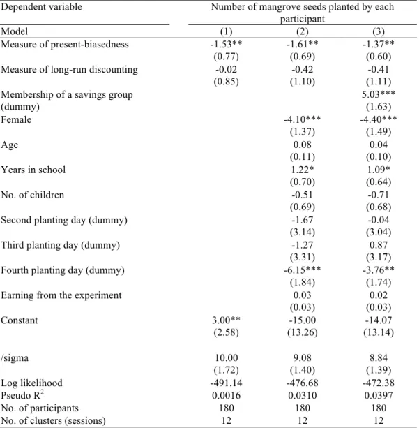
2.11 Appendix G: Tobit regressions for the whole sample of 180 participants

Table 2-6: Tobit regressions of number of mangrove seeds planted by each participant for the whole sample

Dependent variable Number of mangrove seeds planted by each participant

Model (1) (2) (3)

Measure of present-biasedness -1.53**

(0.77)

-1.61**

(0.69)

-1.37**

(0.60) Measure of long-run discounting -0.02

(0.85)

-0.42 (1.10)

-0.41 (1.11) Membership of a savings group

(dummy)

5.03***

(1.63)

Female -4.10***

(1.37)

-4.40***

(1.49)

Age 0.08

(0.11)

0.04 (0.10)

Years in school 1.22*

(0.70)

1.09*

(0.64)

No. of children -0.51

(0.69)

-0.71 (0.68)

Second planting day (dummy) -1.67

(3.14)

-0.04 (3.04)

Third planting day (dummy) -1.27

(3.31)

0.87 (3.17)

Fourth planting day (dummy) -6.15***

(1.84)

-3.76**

(1.74)

Earning from the experiment 0.03

(0.03)

0.02 (0.03)

Constant 3.00**

(2.58)

-15.00 (13.26)

-14.07 (13.14)

/sigma 10.00

(1.72)

9.08 (1.40)

8.84 (1.39)

Log likelihood -491.14 -476.68 -472.38

Pseudo R

0.0016 0.0310 0.0397

No. of participants 180 180 180

No. of clusters (sessions) 12 12 12

Notes: * p < 0.1, ** p < 0.05, *** p < 0.01; Robust standard errors clustered on session level in parentheses

Obs. summary: 61 left-censored observations at decision<=0 119 uncensored observations

0 right-censored observations

26 2.12 Appendix H: Time Preferences incorporated in the standard public

good model

Present-biased preferences can be modeled with a simple functional form of the quasi- hyperbolic discounting or the so-called 𝛽 − 𝛿 model (Laibson, 1997). When we plug it into a standard intertemporal utility function from consumption (𝑥 _% , 𝑥 _%'( ), the total utility function 𝑈 in period 𝑡 takes the following form:

𝑈 _% = 𝑢 𝑥 _% + 𝛽 𝛿 ⁽ 𝑢 𝑥 _%'( ,

<

(=>

(A2.8) where 𝑢(∙) is the utility function from consumption; 𝑡 is the present period; 𝑘 is the time span; captures long-run discounting (a discount factor); and is a parameter for present- biased preference with . corresponds to the case of standard exponential discounting. The one period discount factor between the present and a future period is , while the one period discount factor between two future periods is .

We incorporate time dimension and time preference parameters of the 𝛽 − 𝛿 model to the standard social dilemma situation (adapted from the model in Kocher et al., 2016). This is the utility from the contribution decision in the present period 𝑡 to the public good from which 𝑖 can benefit in the future periods.

𝑢 _% 𝜋 _. = 𝐸 − 𝑐 _. + 𝛽 _. 𝛿 _. ⁽ 𝐺 ∙

<

(=>

. (A2.9)

𝜋 _. is an individual’s monetary payoff, which depends on the public good technology, the relative price of the private good, and on contribution costs to the public good: 𝜋 _. = 𝑓(𝑐 _. , 𝐺 ∙ ) and ^IJ _IL

K

< 0; where 𝐺 is the public good technology; 𝑐 _. ≥ 0 is 𝑖’s contribution to the public good from the available endowment 𝐸 and the rest is for the private consumption.

Assume that every contribution is individually irrational ( ^{IO ∙} _IL

K

< 1), but collectively rational (𝑛 ∙ ^{IO ∙} _IL

K

> 1).

We investigate the relationship between individual contribution to the public good 𝑐 _. and time preference parameters (𝛽 _. , 𝛿 _. ) by looking at the partial derivative of the individual contribution level in present-biased parameter and in the long-run discounting behavior.

The total utility in period 𝑡 from the contribution to the public good:

𝑢 _% 𝜋 _. = 𝐸 − 𝑐 _. + 𝛽 _. 𝛿 _. ⁽ 𝐺 ∙ .

<

(=>

€

δ

€

β

€

0 ≤ β < 1

€

β = 1

€

βδ

€

δ

𝜕𝑢 _% (𝜋 _. )

𝜕𝛽 _. = − 𝜕𝑐 _.

𝜕𝛽 _. + 𝛿 _. ⁽ 𝐺 ∙ + 𝛽 _. 𝛿 _. ⁽ 𝜕𝐺(∙)

𝜕𝑐 _. × 𝜕𝑐 _.

𝜕𝛽 _.

<

(=>

<

(=>

= 0

𝛿 _. ⁽ 𝐺 ∙ + 𝛽 _. 𝛿 _. ⁽ 𝜕𝐺(∙)

𝜕𝑐 _. × 𝜕𝑐 _.

𝜕𝛽 _.

<

(=>

<

(=>

= 𝜕𝑐 _.

𝜕𝛽 _.

𝛿 _. ⁽ 𝐺 ∙ = 𝜕𝑐 _.

𝜕𝛽 _. 1 − 𝛽 _. 𝛿 _. ⁽ 𝜕𝐺(∙)

𝜕𝑐 _.

<

(=>

<

(=>

𝜕𝑐 _.

𝜕𝛽 _. = ^< _(=> 𝛿 _. ⁽ 𝐺(∙) 1 − 𝛽 _. 𝛿 _. ⁽ 𝜕𝐺(∙)

𝜕𝑐 _.

< (=>

With sufficient small number of periods (𝑇) and/or sufficient small long-run discounting parameter 𝛿 _. and/or sufficient small present-biased parameter 𝛽 _. , ^IL

IV

is larger than 0, which indicates that higher present bias (smaller 𝛽 _. ) decrease individual contribution to the public good.

𝜕𝑢 _% (𝜋 _. )

𝜕𝛿 _. = − 𝜕𝑐 _.

𝜕𝛿 _. + 𝛽 _. 𝑘𝛿 _. ^(W> 𝐺 ∙ + 𝛿 _. ⁽ 𝜕𝐺(∙)

𝜕𝑐 _. × 𝜕𝑐 _.

𝜕𝛿 _.

<

(=>

= 0

𝛽 _. 𝑘𝛿 _. ^(W> 𝐺 ∙ + 𝛽 _. 𝛿 _. ⁽ 𝜕𝐺(∙)

𝜕𝑐 _. × 𝜕𝑐 _.

𝜕𝛿 _.

<

(=>

<

(=>

= 𝜕𝑐 _.

𝜕𝛿 _.

𝜕𝑐 _.

𝜕𝛿 _. 1 − 𝛽 _. 𝛿 _. ⁽ 𝜕𝐺(∙)

𝜕𝑐 _.

<

(=>

= 𝛽 _. 𝑘𝛿 _. ^(W> 𝐺 ∙

<

(=>

𝜕𝑐 _.

𝜕𝛿 _. = ^< _(=> 𝑘𝛿 _. ^(W> 𝐺(∙) 1 − 𝛽 _. 𝛿 _. ⁽ 𝜕𝐺(∙)

𝜕𝑐 _.

< (=>

With sufficient small number of periods (𝑇) and/or sufficient small long-run discounting parameter 𝛿 _. and/or sufficient small present-biased parameter 𝛽 _. , _IX ^IL

K

is larger than 0, which indicates that higher long-run discounting (smaller 𝛿 _. ) decrease individual contribution to the public good.

The model thus suggests that as future benefits from the public goods are discounted, 𝑖 contributes less to the public good, the more 𝑖 discounts the future.

Proposition 1: Given constant long-run discounting (𝛿 _. ), higher present bias (smaller

𝛽 _. ) decrease contribution (𝑐 _. ).