The talkative AGN next door

Fakultät Physik – Experimentelle Physik V

The talkative AGN next door

Broad-band spectral variability of the TeV blazar Markarian 501

Dissertation

zur Erlangung des akademischen Grades eines

Doktors der Naturwissenschaften (Dr. rer. nat.)

vorgelegt von

Dipl.-Phys. Marlene Doert

Februar 2013

Contents

1 Introduction 1

2 Astroparticle Physics Briefly 3

2.1 The Messengers . . . . 3

2.1.1 Charged cosmic rays . . . . 4

2.1.2 Cosmic gamma-rays . . . . 5

2.1.3 Neutrinos . . . . 6

2.2 The Processes . . . . 6

2.2.1 Particle acceleration - Fermi I and II . . . . 7

2.2.2 Synchrotron radiation . . . . 7

2.2.3 (Inverse) Compton scattering . . . . 8

2.2.4 γγ-absorption . . . . 8

2.2.5 Photo-hadronic interactions . . . . 9

2.2.6 Electromagnetic cascades . . . . 9

2.3 The Sources . . . . 10

2.3.1 Supernova remnants . . . . 10

2.3.2 Binary systems . . . . 10

2.3.3 Galactic center . . . . 10

2.3.4 Active galaxies . . . . 11

2.3.5 Gamma-ray bursts . . . . 11

2.3.6 Starburst galaxies . . . . 11

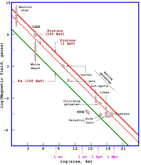
2.3.7 Candidates for CR emission - the Hillas plot . . . . 11

3 Gamma-ray Astronomy with the MAGIC Telescopes 13 3.1 The Imaging Air Cherenkov Technique . . . . 13

3.2 The MAGIC Telescopes . . . . 15

3.2.1 Design/Construction . . . . 15

3.2.2 Operation . . . . 16

3.3 MAGIC Analysis . . . . 17

3.3.1 Analysis goals . . . . 17

3.3.2 Monte Carlo simulations . . . . 17

3.3.3 Data quality selection . . . . 18

3.3.4 Calibration . . . . 18

3.3.5 Image cleaning and characterization . . . . 18

3.3.6 Stereo parameters . . . . 19

3.3.7 Background suppression and energy estimation . . . . 19

i

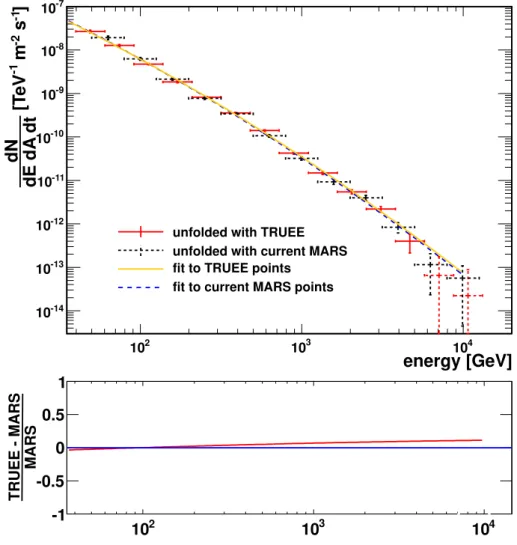
3.3.10 Reconstruction of the energy spectrum . . . . 22

4 TRUEE - Unfolding gamma-ray energy spectra 23 4.1 Unfolding - Definition and Motivation . . . . 23

4.2 Inverse problems . . . . 24

4.3 Unfolding and Regularization . . . . 25

4.3.1 Discretization . . . . 25

4.3.2 Determining the response matrix . . . . 26

4.3.3 Matrix inversion versus unfolding fit . . . . 26

4.3.4 Regularization . . . . 28

4.3.5 Alternative method: Forward Folding . . . . 29

4.4 TRUEE . . . . 29

4.4.1 Parametrization using splines . . . . 30

4.4.2 The response matrix . . . . 30

4.4.3 Choice of observables . . . . 30

4.4.4 Parameter selection . . . . 31

4.4.5 Treatment of background . . . . 32

4.4.6 Acceptance correction . . . . 32

4.4.7 Verification with a posteriori observable distributions . . . . 32

4.4.8 Test mode . . . . 33

4.5 TRUEE Unfolding in MAGIC . . . . 34

4.5.1 Present MAGIC unfolding . . . . 34

4.5.2 Motivation for unfolding with TRUEE . . . . 35

4.5.3 Incorporation of TRUEE in the MAGIC analysis chain . . . . 35

4.6 First application of TRUEE in a MAGIC analysis . . . . 40

4.6.1 Utilized data and Monte Carlo samples . . . . 41

4.6.2 Preparation with made-up: Cuts . . . . 41

4.6.3 Choice of observables . . . . 42

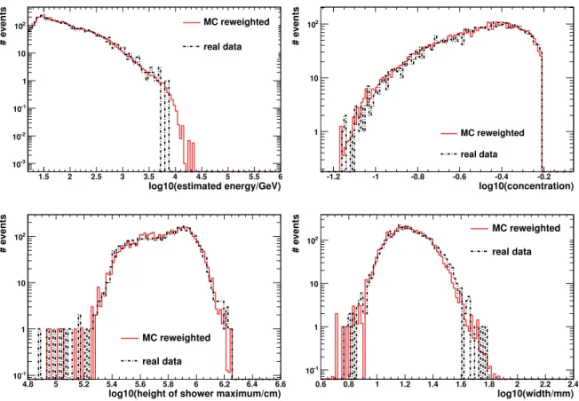
4.6.4 Application on Monte Carlo simulated data . . . . 44

4.6.5 Application on Crab Nebula data . . . . 47

4.6.6 Verification using observable distributions . . . . 49

4.7 Conclusion . . . . 50

5 The Active Galaxy Markarian 501 - a talkative blazar in our neighborhood 51 5.1 Active Galactic Nuclei . . . . 51

5.2 Blazars . . . . 53

5.2.1 Blazar sequence . . . . 54

5.2.2 Acceleration and emission models . . . . 55

5.2.3 Blazars: the secrets they still keep . . . . 56

5.3 Markarian 501 . . . . 57

6 MWL Campaign on Mrk 501 in 2009 59 6.1 Motivation and Introduction . . . . 59

ii

6.2 MAGIC data analysis . . . . 60

6.2.1 Data selection . . . . 60

6.2.2 Off-data sample . . . . 61

6.2.3 Monte Carlo selection and RF training . . . . 61

6.2.4 Flux variability analysis . . . . 63

6.2.5 Spectral analysis . . . . 66

6.3 Multi-instrument data set . . . . 68

6.4 Summary on average state results . . . . 68

6.5 MWL flux variability . . . . 69

6.5.1 Outbursts in the X-ray and VHE band . . . . 72

6.5.2 Variability analysis . . . . 74

6.5.3 MWL correlations . . . . 74

6.6 MWL spectral variability . . . . 76

6.6.1 VHE gamma-rays . . . . 78

6.6.2 X-rays . . . . 78

6.6.3 Evolution of SEDs . . . . 82

6.7 Modeling . . . . 84

6.8 Summary . . . . 88

6.9 Discussion . . . . 89

6.10 Conclusion . . . . 93

7 AGN: Sources of neutrinos and charged cosmic rays? 95 7.1 Motivation and Introduction . . . . 95

7.2 The Process . . . . 96

7.3 The Method . . . . 97

7.4 Application to data . . . . 98

7.4.1 Data selection . . . . 98

7.4.2 Parametrization of the high energy bump . . . . 98

7.4.3 Flux normalization via integration . . . . 98

7.4.4 Resulting neutrino fluxes . . . . 99

7.4.5 How many events could IceCube see? . . . . 99

7.5 Discussion and Conclusion . . . . 100

8 Final Conclusion and Outlook 103

A Cuts for new spectral reconstruction method 105

B MWL analysis of Mrk 501 107

List of Figures I

List of Tables III

Bibliography V

Author’s Publications XIX

iii

Acknowledgment/Danksagung XXIII

iv

Chapter 1

Introduction

Astroparticle physics is a comparably young field of research, which unites scientists from the domain of particle physics and from the area of astronomy and astrophysics. Just after the celebration of its 100 ^th anniversary in the year 2012, astroparticle physics continues to be an active and fast-growing field, which promises not only to provide deeper insights into the most powerful environments within our Universe, but also to deliver results at the interface of searches for new physics in various different fields. Ultimately, this synergy will help us to understand the evolution, constitution and the future of our Universe.

Within astroparticle physics, the field of gamma-ray astronomy can be seen as the natural extension of “conventional” astronomy, which mankind has pursued probably ever since by exploring the night sky with the naked eye or, later on, through the help of telescopes.

In the last century, the accessible part of the electromagnetic spectrum has been expanded beyond visible light by the use of radio telescopes and satellite experiments. Gamma-ray astronomy now allows to probe the very end of the electromagnetic spectrum and can thus give insights into the most energetic phenomena in the Universe. After the technique passed its proof of principle only a few decades ago, the exploration of the gamma-ray sky is now entering a Golden Age, as experiments are at hand which are sensitive enough to allow for deep studies of cosmological objects, such as the black holes sitting at the center of active galaxies.

The work performed in the scope of this thesis has been dedicated to a better under- standing of the phenomenon of active galactic nuclei (AGN). These objects stand out by producing a powerful and highly variable output over the entire electromagnetic spectrum, while being one of the most favored candidates for the sources of the highest energetic cosmic radiation in charged particles. A better understanding of these objects will pave the way for detailed studies of the evolution of the cosmos and the discovery of new fun- damental physics phenomena.

The subject of AGN has been approached via the example of the TeV blazar Markarian 501, which presents itself as the ideal candidate for deep studies of the intrinsic mechanisms at work, by its vicinity and high variability.

The work which is presented in this thesis is anchored in the field of gamma-ray astronomy, as it has been performed within the collaboration of the MAGIC experiment. Still, besides the cooperation with groups exploring the other bands of the electromagnetic spectrum in a multi-wavelength study, the connection to another area of astroparticle physics re- search, namely the field of neutrino astronomy, has been pursued in the context of the multi-messenger approach.

1

The thesis is organized as follows:

Chapter 2 gives a brief overview of the field of astroparticle physics. The different messenger particles are introduced, the relevant basic mechanisms by which they are ac- celerated, produced, deflected or attenuated are outlined and the different types of sources which are currently being studied are briefly discussed.

A preface to the principles of air showers and Cherenkov gamma-ray astronomy is given in Chapter 3, followed by an introduction of the MAGIC experiment. The experimental setup of the two-telescope system as well as the basic analysis procedure are illustrated here.

In Chapter 4, the theme of inverse problems is outlined, followed by an introduction into the method of regularized unfolding. After a brief presentation of the novel unfolding program TRUEE, the incorporation of the program into the standard MAGIC analysis chain is discussed, which has been a major project in the course of this thesis. Sub- sequently, the first application of the new unfolding chain on MAGIC telescope data is presented.

Being one of the major candidates discussed in the preceding chapters, Chapter 5 intro- duces the source class of AGN and blazars in particular, summarizing their observational properties throughout the electromagnetic spectrum. The current state of research and the open questions are outlined. The object Markarian 501, which is subject to two studies which have been performed in the course of this thesis, following quite different approaches, is introduced here.

Chapter 6 presents a multi-instrument campaign on Markarian 501, which has been another major project in the scope of this thesis. At first, the results of an analysis of the corresponding MAGIC data are shown. Subsequently, the multi-instrument data set is discussed, including detailed studies of variability and inter-band correlations, spectral variability and the evolution of the broad-band spectral energy distribution during flaring episodes. The results are discussed in the light of leptonic emission models, based on previ- ous works on this data set, and in the context of similar results seen in other source classes.

Chapter 7 approaches Markarian 501, and the blazar class in general, from a contrary point of view, assuming hadronic interactions and the consequential production of neutri- nos. An estimation for a possible neutrino signal from such processes is pursued, while only simple bolometric considerations are used. The results, which are obtained on the basis of the data set presented in the preceding chapter, are discussed in the context of state-of-the-art neutrino astronomy.

After detailed discussions of results and conclusions are given at the end of the respective

chapters, Chapter 8 concludes the thesis and provides a brief outlook to possible future

activities based on the presented work.

Chapter 2

Astroparticle Physics Briefly

The first step into the field of astroparticle physics was taken by V. Hess in 1912, when he discovered that ionizing radiation, which he called Höhenstrahlung, is reaching us from space [Hes12]. Further findings which were linked to measurements of astroparticles, like the discovery of the muon, the pion and the positron, have had great influence on the development of particle physics. Nowadays, astroparticle physics has emerged to be a vivid, still young, field of research. It has grown to be an advantageous combination of astrophysics and particle physics, from which both “parent” fields substantially profit.

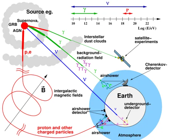
The possible channels to study astrophysical sources have been expanded by very high energy photons, neutrinos and potentially charged particles such as the highest energy protons. These new messengers give access to the most powerful phenomena in our Uni- verse, and will contribute to understanding extreme events such as supernova explosions and gamma-ray bursts, but also the fascinating phenomenon of black holes, their influence on the formation of galaxies and ultimately the formation of the Universe that we know today.

On the other hand, cosmic accelerators can be exploited to study particle physics at energy scales beyond anything possible to establish in man-made machines. Once the sources of the highest energy cosmic rays are found and a reasonable understanding is acquired, they could be promising cosmic laboratories which offer accelerated particles at outstandingly high energies and even “for free”, while of course posing the challenge of an uncontrollable and probably unpredictable particle beam.

For a detailed introduction into the field of astroparticle physics, see for example [FR12]

and [BG06], which served as the basic references for the following sections.

2.1 The Messengers

The messenger particles which are addressed in the context of astroparticle physics, namely the charged cosmic rays, highest energy photons and neutrinos, have very different char- acteristics, which give them distinct advantages (and disadvantages) for studying different aspects of the highest energy phenomena. In the following, a short overview of the particles and their major properties is given.

3

00000000 00000000 0000 11111111 11111111 1111 000000 000000 000 111111 111111 111

B

10 12 14 16 18 20 22

Log (E/eV)

γ P

ν

µ µ

γ

ν

ν

Supernova,

γ γ

ν

p,e

γ γ γ γ

γ γ γ

Interstellar

dust clouds experiments

Cherenkov−

detector background−

satellite−

Earth

detector underground−

detector intergalactic magnetic fields

Atmosphere airshower

airshower

airshower proton and other

charged particles

radiation field GRB

AGN

Source eg.

Figure 2.1: Schematic overview of multi-messenger astrophysics: emission in charged par- ticles (p, e), high energy photons (γ) and neutrinos (ν) is emitted from a particle accelerating source (for a discussion of the sources see section 2.3).

The particles propagate through space where they are perturbed by magnetic fields (p, e), clouds and background radiation (p, e and γ) or not at all (ν), until they are detected in one of the various experiments in the Earth’s orbit, on the surface or underground. The typical energies of the particles are also indicated. Figure: [Dre10] after [Wag04].

2.1.1 Charged cosmic rays

After an incoming flux of charged particles has been found by V. Hess in 1912, the term cosmic rays (CR) was coined by R. A. Millikan in 1925 [MC28]. To distinguish these par- ticles from the very high energy photons, which also contribute to the cosmic radiation (see Sec. 2.1.2), they are nowadays also referred to more precisely as charged cosmic rays.

The population of particles which enter the atmosphere are made up by 98% of light atomic nuclei (at energies > 1 GeV). At these energies, charged leptons contribute only by

≈ 2%, cf. [BG06].

The spectral distribution of cosmic ray particles spans up to 13 orders of magnitude in

energy. Its shape is essentially a power-law, with two spectral breaks at 10 ¹⁵ -10 ¹⁶ eV (the

so-called knee) and at 10 ¹⁸ -10 ¹⁹ eV (the ankle). The corresponding spectral indices are -2.7

2.1 The Messengers 5

before the knee, a steepening to -3.0 above, and a flattening after the ankle, cf. [BG06]. At energies above 4 · 10 ¹⁹ eV, the particles have enough energy to interact with ambient pho- tons of the cosmic microwave background (CMB), see [PW65]. This phenomenon is known as the Greisen-Zatsepin-Kuzmin (GZK) cutoff, which was predicted in 1966 [Gre66,ZK66].

Recent measurements confirm a suppression of the flux at these energies [A ⁺ 08a]. For more details see also [FR12].

Being electrically charged, CR particles interact with interstellar and intergalactic mag- netic fields. Due to multiple deflections in these fields, the particle flux is isotropized and generally no information can be gained about the origin of the particles.

The breaks in the spectrum might be hints to possible limitations of different accelerat- ing mechanisms or populations of sources. Particles which contribute to the flux at the highest energies are likely to stem from outside the Milky Way, as the galactic magnetic fields cannot confine particles with gyroradii corresponding to such energies [Lin63]. The question of the sources of CRs in this energy range is one of the crucial puzzles in the field today. Several source classes (and single sources) beyond our galaxy have been suggested as good candidates for this emission, see e.g. [BS12, TH11, DR10].

Due to the same effect, particles at the highest energies (the so-called sub-GZK particles), are crucial to be studied, as they are less deflected during propagation through space and should point back to their sources. The low particle flux, which governs this energy range, requires elaborate detection techniques in order to acquire the necessary amount of events, such as the Auger experiment, which combines particle detectors and fluorescence telescopes to a 3000 km ² sized hybrid experiment [A ⁺ 08a].

2.1.2 Cosmic gamma-rays

Another part of the cosmic radiation is formed by photons which populate the high en- ergy end of the electromagnetic spectrum, the gamma-rays (E & 1 MeV). Due to their electromagnetic neutrality, gamma-rays are not deflected by magnetic fields during their propagation. Therefore, they can be used to perform source studies, which has led to the new field of gamma-ray astronomy. However, at the highest energies these photons undergo attenuation by interactions with low energy photons, which fill up the Universe.

This background field, which is formed by the accumulation of star light and radiation from dust, is commonly referred to as the Extragalactic Background Light (EBL). Models are at hand which describe the distribution of low energy photons and the resulting atten- uation factors as a function of energy and source distance, see e.g. [SDJS92,KD10,FRV08].

As the EBL has a direct relation to the evolution of the Universe itself, gamma-ray spectra of cosmological sources are used to study the composition and evolution with time and distance of the EBL.

The detection of gamma-ray photons is hindered by the fact that, unlike photons in the optical or the radio regime, they are absorbed by the atmosphere. Satellite missions such as the Energetic Gamma Ray Experiment Telescope (EGRET) [K ⁺ 89] and now the Fermi Gamma-ray Space Telescope (Fermi -GST) [A ⁺ 09c] are used to probe the flux in gamma- rays from outside the Earth’s atmosphere. Due to the limits in detector size, however, combined with steeply decreasing statistics towards higher energies, only the range up to

≈ 300 GeV can be accessed with these instruments. In the regime of very high energies

(E & 50 GeV), the imaging atmospheric Cherenkov technique offers to use the atmosphere

as a detection volume, by observing so-called extensive air-showers which are initiated by the gamma-ray photons. Chapter 3 will give more insight into ground-based gamma-ray astronomy and introduce one of the state-of-the-art experiments in the field, the MAGIC telescopes [A ⁺ 12a].

2.1.3 Neutrinos

The third species of cosmic messenger particles are neutrinos - neutral, very light leptons.

Due to the fact that they interact only via the weak force, neutrinos are able to travel over large distances without being deflected or attenuated. And while photons (and hadrons) might be trapped in central regions of stars or within the sites of particle acceleration and production, neutrinos can easily escape. These characteristics make them ideal messengers in order to probe the center of objects in far distances which are opaque to other kinds of emission.

Neutrinos are produced in hadronic interactions, e.g. in the fusion of atomic nucleii at the center of the sun or as a decay product of particles created in interactions of relativistic hadrons with photon fields or among themselves.

During their propagation in space, neutrinos undergo oscillations between the different fla- vor states (ν _e , ν _µ , ν _τ ). This effect was found as the solution to the solar neutrino problem, which was phrased after a too small flux in ν e was measured from the sun [BD66, GP69].

The confirmation of these oscillations can be seen as the first correction to the standard model of particle physics (SM), as oscillations require neutrinos to have a finite mass, which is not foreseen in the SM.

After studies of astrophysical neutrinos in absorption experiments (e.g. Homestake [C ⁺ 98]

and GALLEX [Vig98]) and scattering experiments (such as (Super-)Kamiokande [F ⁺ 98b]), which utilized detection volumes such as water tanks for their measurement, experiments of a new type have been set up in order to detect cosmic neutrinos at the highest energies.

The steeply decreasing event numbers at very high energies and the small cross-section of the interactions themselves required much larger detector volumes and led to the ex- ploitation of natural water or ice environments, such as a lake (BAIKAL [B ⁺ 97a]), the sea (e.g. ANTARES [A ⁺ 11d]) and the antarctic ice (first AMANDA [A ⁺ 00], currently IceCube [A ⁺ 06a]). The biggest challenge for these experiments is the suppression of a vast background of neutrinos which are induced in interactions of charged CRs in the atmosphere. So far no detection of cosmic very high energy (VHE) neutrinos could be claimed.

2.2 The Processes

In the following, the processes of particle acceleration and interaction which are relevant

for this work are outlined briefly. For a very recent overview and detailed explanations on

the processes introduced below, see for example [FR12] and [BHK12], but also [RL08].

2.2 The Processes 7 2.2.1 Particle acceleration - Fermi I and II

E. Fermi was the first to postulate the idea that CRs might be produced by collisions of particles with magnetized interstellar clouds [Fer54]. This stochastic acceleration involves terms with O(∆v ² ), where ∆v is the differential of the involved velocities, and is therefore also known as second-order Fermi acceleration.

Later on, this principle was applied to shock environments, see [Kry77, ALS77, Bel78a, Bel78b, BO78], which yields a process that is linear in the velocity differential (O(∆v)), and is thus much more efficient. This diffusive shock acceleration is therefore also referred to as first-order Fermi acceleration. Like the stochastic acceleration, this process leads to power-law distributions of the resulting particle spectra. In the non-relativistic case, the spectral index only depends on the shock compression, e.g. the ratio between the plasma velocities upstream and downstream of the shock. In the case that the shock moves at relativistic speed, see e.g. [K ⁺ 00a], it depends on the upstream flow speed, orientation of the magnetic field with respect to the shock and the characteristics of the involved scattering processes. Typically, indices around −2 are realized. Fermi acceleration at relativistic shocks is thought to take place within relativistic jets in astronomical objects.

For a descriptive discussion of the processes see e.g. [FR12] and [BHK12].

2.2.2 Synchrotron radiation

Charged particles which are moving within a magnetic field generally follow a spiral path.

This means that they are constantly deflected or accelerated. In the relativistic case, they will emit synchrotron radiation, which can be understood as the relativistic generalization of cyclotron radiation. This highly polarized radiation can span over a broad spectrum, while the spectral index of the photon distribution is closely related to the distribution of the emitting particles. Discussing the energy distribution of the accelerated particles n(γ), energies are described in terms of the particle Lorentz factor γ , corresponding to

γ = 1

p 1 − β ² , with β = v

c . (2.1)

For a particle distribution

n(γ) = n ₀ γ ^−p , (2.2)

which is characterized by a spectral index p (while n ₀ represents a normalization factor), this results in a synchrotron spectrum which, over a wide range in ν, follows

j(ν) ∝ ν ^{−α sy} , with α _sy = p − 1

2 , (2.3)

combined with a low and a high energy cutoff, cf. [BHK12]. Here, ν denotes the photon frequency, j(ν) is the spectral distribution of the photons and α sy defines the synchrotron spectral index. Naturally, the spectra become more complicated for more detailed particle spectra.

Due to this so-called synchrotron cooling, the radiating particle loses energy, while the particle energy-loss rate strongly depends on the mass (m) of the particle:

dγ dt sy

∝ −m ⁻³ , (2.4)

see [BHK12] for a more detailed expression. This makes electrons radiate much more efficiently than heavier particles, but it also implies that they cool fast and acceleration to the highest energies is problematic. Protons or heavier nuclei radiate less efficiently, but can be accelerated to very high energies more easily.

A part of the produced synchrotron photons may be absorbed again during interac- tions with the relativistic electrons, which leads to an effect known as synchrotron self- absorption. The corresponding absorption probability is dependent on the magnetic field and the photon frequency itself. Consequentially, the regions of such synchrotron radia- tion may be opaque (with an optical depth τ ≥ 1) below a critical frequency ν SSA . For detailed calculations and illustrations of the resulting spectrum see e.g. [BHK12].

2.2.3 (Inverse) Compton scattering

Electrons (and positrons) can undergo Compton scattering processes with photons, which are in the general case described by the Klein-Nishina cross-section, see e.g. [JR76,Hei54].

For small photon energies, the process can be approximated by the constant Thomson cross-section, which describes an elastic scattering in the rest frame of the electron.

Such scattering interactions are thought to occur in astrophysical regions of particle ac- celeration, which are typically filled with relativistic electrons and dense photon fields. In the following, photon energies are denoted in units of the electron rest mass:

≡ hν

m e c ² , (2.5)

while the electron energy is denoted in terms of its Lorentz factor γ .

In the so-called Thomson regime (at low photon energies), the photon’s energy after scat- tering is given, in the rest frame of such an emission region, by

scat ≈ γ ² , (2.6)

while describes the energy of the photon before scattering, cf. [BHK12]. The photon re- ceives a boost in energy from the electron. As the direction of energy transfer is contrary to the commonly known Compton scattering, this process is also referred to as inverse Compton scattering.

In the Klein-Nishina limit, where γ & 1, the cross-section for the process is strongly suppressed. This makes the upscattering of high energy photons much less efficient.

It can be shown that the (inverse) Compton spectrum is characterized by the same spec- tral index α C = α sy , which was obtained for the synchrotron spectrum, if a power-law distribution of electrons and a monoenergetic photon field are assumed [BHK12]. See this reference also for detailed calculations of the cross sections, including also its angular dependence.

2.2.4 γγ-absorption

Photons of different energies 1 and 2 can interact with each other and produce an

electron-positron pair. This is true for high energy gamma-ray photons among themselves

2.2 The Processes 9

and with low energy photons, as long as the relevant energy threshold ₁ ≥ 2

2 (1 − µ) (2.7)

is surpassed. Here, µ = cos(Θ) describes the collision angle, cf. [BHK12]. These processes are important for interactions of high energy gamma-ray photons with photon fields of lower energy, such as e.g. radiation from the surrounding accretion disk in the vicinity of a plasma jet, which will be discussed in chapter 5.

Besides interactions within the sources of the emission themselves, very high energy gamma-rays can interact with photons of the EBL. The corresponding optical depth τ _γγ increases with gamma-ray photon energy and with the distance of the source.

2.2.5 Photo-hadronic interactions

Hadronic particles are thought to be present, for example, in plasma jets (see section 5.1) and can be accelerated to relativistic energies. In these environments, they can interact with present photon fields via a number of different processes.

Protons and heavier nuclei can interact with the ambient photon field to create elec- tron/positron pairs via Bethe-Heitler Pair production [BH34]. However, it is found that photo-hadronic processes are more dominant in the scenarios discussed in the course of this thesis (e.g. relativistic plasma jets). For a thorough treatment on these interactions see e.g. [BHK12].

In so-called photomeson production processes, the interaction of protons or nuclei with the photon field can create mesons, predominantly pions, following four different channels:

the excitation and subsequent decay of resonances, the direct pion production without involved resonances, diffractive scattering and multi-pion production, cf. [BHK12]. In the

∆−approximation, only the largest resonance ∆(1232) is considered for the production of mesons, which leads to branching ratios of the neutral pion π ₀ to the charge pion π ⁺ of 2:1.

As mentioned above, this process leads predominantly to the production of pions, while the decay into other mesons (mainly K and η) contribute by less than 20%, cf. [BHK12].

A neutral pion decays further into two (very high energy) photons, while a charged pion decays into a muon and a neutrino and further into an electron/positron and two more neutrinos. In chapter 7, these interactions will be treated in more detail in the light of the mentioned approximations.

2.2.6 Electromagnetic cascades

In opaque regions, photons are likely to interact with the present photon field via various

processes, producing electrons/positrons, which themselves result again in the production

of photons and so on. In these so called cascades, the photon energy is gradually repro-

cessed towards lower energies. As several different processes are involved and interlinked,

these cascades cannot be described in a trivial way. Connected to the size of the emission

region, the processes can be differentiated into “saturated cascades”, where more photon

interactions take place than photons escape the region, and “non-saturated” cascades,

where the typical escape time is lower. While the former type generally leads to power-

law distributions with spectral indices α γ → 2, the cascades of the latter type tend to

terminate after a few cycles, cf. [BHK12].

2.3 The Sources

In the following, some of the most interesting sources for the production of high energy radiation - gamma-rays and neutrinos, but possibly also charged CR - will be introduced briefly.

2.3.1 Supernova remnants

Within our galaxy, super nova remnants (SNR) make up one of the most interesting source classes for the detection of astroparticles. The most prominent representative is the Crab Nebula, which is the remnant of a super nova that has been observed by Chinese astronomers in 1054. After the core of a massive star collapses because of a depletion in the fusion material, its outer material is ejected into the interstellar medium, producing shocks and excellent sites for particle acceleration. While the core might form a neutron star (possibly a pulsar) or a black hole, the remaining outer shells of the former star are referred to as a SNR. In the case of a rotating neutron star at the center of the object, the remnant is called a pulsar wind nebula (PWN). Typically, SNR exhibit very hard spectra in gamma-rays, which are cutoff only at energies of about 20 TeV. This indicates that the accelerated particles, which are responsible for the emission of gamma-rays, must feature energies up to 10 ¹⁴ or even 10 ¹⁵ eV, cf. [FR12]. SNRs are thought to make a substantial contribution to the observed flux of charged CRs below and possibly also above the knee, see also [Dru12].

2.3.2 Binary systems

Another promising class of sources are binary systems, which contain a compact remainder of a former massive star (either a black hole or a neutron star). These systems are characterized by accretion of matter onto the compact object, which might exhibit outflows of relativistic particles in the form of plasma jets, cf. [FR12] and also chapter 5. Such systems are referred to as micro quasars.

2.3.3 Galactic center

A region which is densely populated, and probably hosts many different classes of promis- ing candidates for high energy emission, is the Galactic center. However, given the large density of emitters, the detection and investigation of single sources is challeng- ing. Within the most prominent feature in this region, Saggitarius (Sgr) A, possibly a super-massive black hole has been identified (Sgr A*), which is also an emitter of VHE gamma-rays [KT12,A ⁺ 04], cf. [FR12].

As a center of mass accumulation, the Galactic center is also a good candidate for searches

for dark matter (DM) annihilation or decay signatures. Gamma-rays could be produced as

a product of these processes. However, the hard spectrum seen from this region suggests

the dominant emission to come from PWN rather than dark matter annihilation/decay,

cf. [FR12].

2.3 The Sources 11 2.3.4 Active galaxies

Beyond our galaxy, radio galaxies, quasars and a large number of different source classes, which are seen in radio, optical, X-ray and higher frequencies, have been summarized as Active Galactic Nuclei (AGN). These objects, which host a super-massive black hole that is fed by surrounding material, are thought to (partly) exhibit highly relativistic particle outflows, which are the sources of VHE gamma-rays and possibly also of the highest energy CRs. The source class of AGN and the subclass of blazars will be introduced in more detail in chapter 5.

2.3.5 Gamma-ray bursts

Spontaneous, very rapid outbursts in gamma-rays have been detected, which subside again after few seconds, but leave a so-called afterglow in optical, radio and X-ray frequencies, which can be visible over weeks. These transient objects have been named gamma-ray bursts (GRB) and are thought to be caused by core-collapse supernovae and/or colliding neutron stars, cf. [BG06]. GRBs constitute one of the most promising source classes for the emission of the highest energy CRs.

2.3.6 Starburst galaxies

Starburst galaxies are a subclass of galaxies, which show no core activity like AGN, but still exhibit TeV gamma-ray emission (for an overview and a recent discussion see e.g. [Ohm12, LT12]). The large abundance of supernova events leads to strong stellar winds within these galaxies, which are thought to be sites for particle acceleration, cf. [FR12].

2.3.7 Candidates for CR emission - the Hillas plot

While supernovae are discussed as the best candidates for the production of charged cosmic rays at intermediate to high energies, the sources for the highest energy CRs are still looked for. In 1984, M. Hillas discussed the properties which give a source class the capability to accelerate particles up to such high energies. The potential of a source depends on the size of the emitting region and the strength of the prevailing magnetic fields (B ), in combination with the charge (Ze) and energy (E) of the particles themselves. In the scope of gradual acceleration models, the size of the accelerating region L has to be much larger than the particle’s Larmor radius

r L ∝ E

ZB , (2.8)

in order to keep particles in the process. Taking into account scattering processes and the relativistic velocity of the scattering centers β, the following condition has to be fulfilled:

BL > 2E

Zβ , (2.9)

where B is given in µG, L in pc and E is quoted in 10 ¹⁵ eV, cf. [Hil84]. In the so-called

Hillas plot (see Figure 2.2), possible candidates for the acceleration of protons and heavier

Figure 2.2: The Hillas plot: overview of candidate sources (or regions within sources) for the emission of the highest energy CR, based on their size and the prevailing magnetic field. Objects below the respective diagonal lines cannot accelerate particles to the given energies. While particular regions in AGN could be responsible for the emission of protons up to ≈ 100 EeV, GRB or neutron stars might be the sources of ultra high energy CRs at around 1 ZeV. For more details, see text. Figure: [Str09], adapted from [Hil84].

nuclei of different energies can be identified.

Currently, AGN jets (or so-called hot spots therein) are still favored, before GRBs, as

emitters of the highest energy cosmic rays, see e.g. [B ⁺ 09a, Der11]. In chapter 5, these

interesting and promising objects will be introduced and discussed in more detail.

Chapter 3

Gamma-ray Astronomy with the MAGIC Telescopes

The gamma-ray spectrum which reaches Earth from a - meanwhile large - number of sources is being explored from MeV energies up to several tens of TeV. However, above

≈ 100 GeV, the steep spectrum does not allow to acquire sufficient statistics with space- bound experiments, which are limited in the size of the detection area. Still, gamma events are absorbed in the Earth’s atmosphere and do not reach the surface. While this does not permit to measure gamma-ray photons directly with ground-based detectors, this fact is being exploited by the imaging air Cherenkov technique. The observation of so-called air showers, which are induced by gamma-ray events, still allows to observe such events with ground-based telescopes and at the same time offers a huge increase in events statistics, as the whole atmosphere is turned into a detection volume. In this chapter, this observation technique will be briefly discussed. Subsequently, the MAGIC telescopes will be introduced, which are a state-of-the-art ground-based gamma-ray imaging facility, and the basic principles of an analysis of MAGIC data will be outlined.

3.1 The Imaging Air Cherenkov Technique

When highly energetic particles (gamma-rays as well as charged CRs) enter the atmo- sphere, they interact with the atmospheric particles and induce a cascade of secondaries.

This cascade increases rapidly, as long as the remaining energy per shower particle is high enough to undergo further interaction. This “cloud” of highly energetic particles is referred to as an extensive air shower. The size and elongation of such a shower is de- pendent on the energy of the primary particle. Gamma induced showers typically show a slim, spindle-shaped structure, while showers which are induced by hadronic particles fea- ture a broader transversal spread and a more heterogeneous composition, as the contained hadronic secondary particles can cause electromagnetic sub-showers at different positions, further away from the shower axis. Typical hadronic and photon-induced cascades, which have been simulated with the Monte Carlo program CORSIKA (see subsection 3.3.2), are shown in Figure 3.1. Compared to gamma-ray showers, hadronic events of this kind are much more abundant (by at least a factor 10 ³ ) and pose a strong background to gamma- ray measurements.

As the particles which form such an air shower are highly energetic and move with a ve- locity that is larger than the speed of light in the surrounding air, they emit Cherenkov

13

Figure 3.1: Monte Carlo simulated air showers: Shown are cascades induced by a gamma particle (left), a proton (middle) and an iron nucleus (right). All particles have been simulated with an energy of 1 TeV, entering the atmosphere perpendicular to the Earth’s surface (zenith angle = 0 ^◦ ) and undergo their first interaction at a height of 30 km. Figure: [Sch13].

radiation. This effect creates a cone of blue to ultra-violet light, which is emitted by the shower in forward direction and can be detected by ground-based telescopes. For a more detailed introduction into the physics of air showers see e.g. [Wee03], but also [FR12]

or [BG06].

After the first detectors which recorded the light emitted by gamma-ray induced air show- ers were built as early as 1953 [GJ53], the idea of an imaging technique was introduced in 1977 [WT77], cf. [FR12]. With the Whipple telescope, the first detection of gamma-rays from a cosmic source has been achieved in 1989 [Wo89], which made the Crab Nebula (a SNR) the first source in the VHE gamma-ray sky. After Whipple and the first stereoscopic imaging air Cherenkov telescope (IACT) array HEGRA (abbrev. for High-Energy-Gamma- Ray Astronomy), currently several Cherenkov telescope systems are in operation, namely the Very Energetic Radiation Imaging Telescope Array System (VERITAS, in Arizona, US) [H ⁺ 06], the High Energy Stereoscopic System (H.E.S.S., in Namibia) [H ⁺ 03] and the Major Atmospheric Gamma-ray Imaging Cherenkov telescopes (MAGIC telescopes, on La Palma de Canarias, Spain) [A ⁺ 12a].

While the next generation of ground-based gamma-ray astronomy instruments is already

being planned, namely the Cherenkov Telescope Array (CTA) project, which will com-

3.2 The MAGIC Telescopes 15

prise of the order of 100 Cherenkov telescopes of different sizes [A ⁺ 11c], the work which is subject to this thesis has been mainly based on measurements obtained with the MAGIC telescope(s).

3.2 The MAGIC Telescopes

Figure 3.2: Photograph of the MAGIC telescopes on the Roque de los Muchachos in La Palma de Canarias [Wag09].

The MAGIC telescopes are a stereoscopic system of two Cherenkov telescopes, which are situated on the Roque de los Muchachos (28.8 ^◦ N, 17.8 ^◦ W, 2,225 m above sea level) in the Canary Island of La Palma, Spain. The telescope has started scientific operation as a stand-alone telescope in 2004 [A ⁺ 08c] and was upgraded to a two-telescope stereo-system in 2009 [A ⁺ 12a].

3.2.1 Design/Construction

The telescopes are characterized by large mirror dishes of 17 m diameter, which are built from aluminum mirrors (while partly also glass mirrors were used for the second telescope dish) and feature a parabolic shape. The single mirrors can be aligned with an active mirror control system. The large mirror dishes increase the amount of light that can be collected with the telescopes, and thus allow also for faint air showers, induced by low energy gamma events, to be recorded. This way, a lower energy threshold of ≈ 50 GeV (in stereo operation) is achieved [A ⁺ 12a].

In order to have a fast-moving telescope, despite its extraordinary size, the telescope frames

have been built from ultra-light carbon-fiber tubes. This allows for fast repositioning of

the telescope, requiring only 20 seconds for a 180 ^◦ turn in azimuth [B ⁺ 09b].

The initial camera of the first telescope (hereafter M1) has been build in a hexagonal shape, of two different types of photo multiplier tubes (PMTs): 397 PMTs with a diameter of 0.1 ^◦ have been placed in the inner part of the camera, surrounded by 180 outer pixels of a diameter of 0.2 ^◦ . The second telescope (hereafter M2) is equipped with a round, ho- mogeneous camera, built from 1039 pixels of 0.1 ^◦ diameter [BT ⁺ 09]. Both cameras have a diameter of 3.5 ^◦ . For calibration purposes, each camera has a so-called calibration box, which supplies short calibration pulses during dedicated calibration runs and in between the data taking runs, to allow for a calibration of the individual pixels later on, see [S ⁺ 02].

In 2012, when the MAGIC system was again upgraded in order to become more homoge- neous, a new M1 camera was installed, which has essentially the same features as the M2 camera.

After conversion of the PMT signals from electric to optical, using vertical cavity laser diodes (VCSELS), and transmission through optical fibers, they are split and fed into the trigger and the read-out system in the counting house.

Different read-out systems were in use for M1. The system which was last used in mono mode and for the first years of the stereo operations was built from flash analog to digital converters (FADCs) [G ⁺ 08]. For M2, a system of domino ring sampler 2 (DRS2) chips was first used. Both systems operated at a sampling rate of 2GSample/s. In the course of the upgrade of the system in 2012, both telescopes are now equipped with DRS4 based read-out systems.

The trigger criterion for an event to be recorded consists of several steps. Each pixel is regulated by a discriminator threshold (the so-called level-zero trigger). The subsequent level-one-trigger requires an X next-neighbor (XNN) criterion to be fulfilled, which means that an event only passes the trigger if a compact group of X pixels passes the discrim- inator. For mono observations, usually a 4NN configuration has been applied, while for stereo observations, 3NN topologies in the single telescopes proved to deliver the best per- formance. In stereo observation mode, an additional stereo trigger “distills” those events, which have been seen in both telescopes [P ⁺ 08]. For a detailed description of the MAGIC stereo system see [A ⁺ 12a].

3.2.2 Operation

During the observation, background events stemming from hadronic showers, the light of

the night sky or from diffusive electrons and gamma-ray particles contaminate the collected

data sample. Although elaborate techniques are used to remove such events, still some

background remains in the measurement. To get a good estimate of the contribution of this

background, off-measurements are required. A practical way to obtain such background

measurements is the so-called Wobble observation mode [Fo94], which permits to observe

the signal region and a background region at the same time. This is achieved by pointing

the telescopes not directly to the source, but to a position in a distance of 0.4 degrees next

to the source. This way, an on-source region and one or several off (source) regions can

be defined in the camera. Alternatively, separate on-source and off-source measurements

are performed and combined later in the course of the analysis.

3.3 MAGIC Analysis 17

3.3 MAGIC Analysis

3.3.1 Analysis goals

The analysis of MAGIC data is generally performed using the standard analysis package MARS [M ⁺ 10b].

Besides the mere detection of a gamma-ray signal from a source, the MAGIC analysis allows also to obtain the distribution of the gamma-ray flux vs. energy, the energy spectrum, the evolution of flux with time, which is referred to as the light curve, and the arrival directions of gamma-ray events in two coordinates, the so-called skymap. While deriving energy spectra is one of the key problems which are addressed in this thesis, and the analysis presented in chapter 6 makes use of both, energy spectra and light curves, no skymaps have been generated in the course of this thesis and will thus not be considered in the following.

3.3.2 Monte Carlo simulations

Owing to the indirect measurement technique, simulations of air shower events and the response of the telescope system are required in order to reconstruct the intrinsic properties of the recorded shower events, such as the type of the incident particle or its energy. These events are simulated following the Monte Carlo (MC) method and are, in the case of MAGIC, generated in three steps: The simulation of the first interaction of the incident particle, the resulting particle cascade and the corresponding Cherenkov light emission are simulated with the air shower simulation program CORSIKA [HKC ⁺ 98]. Subsequently, the program reflector performs the absorption of Cherenkov photons in the atmosphere on their way to the telescope level, the reflection on the telescopes’ mirror surfaces and determines which of the photons reach the camera plane. Details can be found in [Mor02].

Finally, the camera program simulates the response of the PMTs and the electronic system, including the characteristics of the read-out and the trigger. For details see [Bla01].

Following the energy spectral shape which is generally expected from the observed sources,

the underlying spectrum of the incident particles is generated as a power-law distribution,

while the range and the spectral index can be adjusted. Beside the general tuning of

the telescope parameters for the MC, in order to resemble the features of the system

as closely as possible, several parameters have to be adjusted based on the observational

circumstances under which the corresponding data have been taken. Generally, simulations

are generated for several combinations of these parameters, from which the best matching

ones are subsequently chosen for a particular analysis. Alternatively, dedicated simulations

can be generated, which are specifically “tailored” to the data set at hand, see [DH12,

Doe09]. Among the crucial parameters is the range of the covered zenith angles, which is

defined as the angle between the telescope’s pointing position and the zenith position in

the sky. Closely connected to this observation angle is the maximum impact parameter,

which defines the furthest distance from the telescope (system) up to which showers are

produced. The impact parameter itself is measured as the distance between the shower

axis and the telescopes, projected to the ground. Another important parameter which has

to be chosen carefully based on the data sample is the point spread function (PSF) of the

optical system. According to the image defects introduced by the mirrors, this effect is

also simulated in the Monte Carlo. The PSF is defined as a Gaussian spread in the x − y plane of the camera.

3.3.3 Data quality selection

Prior to the actual data analysis, the data sample has to be selected according to several quality criteria, to ensure that technical defects as well as bad weather conditions do not corrupt a reliable analysis result. The general criteria for this quality selection comprise a tolerably stable trigger rate and a not too high direct current (DC) of the signal. The latter would indicate too much light from the night sky, which enters the measurement as noise. Regarding the weather condition, the cloudiness is constantly measured by a pyrometer and should not exceed a given limit. Furthermore, the starguider evaluates the night sky and monitors the number of identified stars. A too low number is also a good indication for poor view and thus bad data quality. For an exemplary choice of values for the parameters see subsection 6.2.1.

3.3.4 Calibration

Based on the calibration runs, which are taken before each data run and interlaced during the normal data-taking procedure, conversion factors (from signal amplitude to number of photo electrons (phe)) are determined for each pixel. PMTs for which the signal amplitude or the arrival time has been reconstructed wrongly are interpolated, cf. [A ⁺ 08c]. This step is performed with the program callisto or, since the upgrade of the telescope system in 2012, with sorcerer. This is performed for both, real data and MC.

3.3.5 Image cleaning and characterization

Subsequent to the calibration, a cleaning procedure is applied, which allows to remove all pixels from the camera image, that do not belong to the image of the shower. To achieve this, two cleaning levels are defined: The higher threshold (typically 6-10 phe) specifies so-called core pixels. A lower threshold is applied (in general about 3-5 phe), which leaves pixels with a content above this level in the image, if they are adjacent to a core pixel.

After this procedure, only the image of the shower remains, which is typically of an elliptical shape (but can look more complicated for hadronic showers and showers of higher energy in general). Subsequently, these shower images are characterized by a number of parameters, so-called image parameters [Hil85]. Among these are the parameters width and length, which describe the semiaxes of an ellipse given by the root mean square (RMS) of the 2-dimensional light distribution (see left panel of Figure 3.3). In this context, the parameter α describes the angle between the major axis of the ellipse and the connecting line between the center of gravity of the ellipse and the defined source position in the camera (see also Figure 3.3). Further parameters describe other properties of the image, e.g. the light content of the shower (size), the concentration of the light distribution (conc) and the number of islands, which is defined as the number of discontiguous light patches.

These two tasks are performed using the program star, which is also applied to simulated

and real data.

3.3 MAGIC Analysis 19

Figure 3.3: Schematic views of the definition of image parameters in the camera plane.

Left panel: Basic image parameters proposed by M. Hillas [Hil85]. Figure from [A ⁺ 08c]. Right panel: Reconstruction of the source position using the Disp method [L ⁺ 01,DS ⁺ 05]. Figure from [Maz07].

3.3.6 Stereo parameters

In the case of stereo observations, the program superstar merges the data from the two telescope pipelines and allows to determine the impact parameter (see subsection 3.3.2) and the maximum height of the shower for each event. These parameters are obtained based on the stereoscopic information and can improve the energy estimation and the suppression of the background [Feg97], see also [A ⁺ 12a].

3.3.7 Background suppression and energy estimation

The sought-for gamma-ray events are dominated by a huge background of hadronically- induced shower events by about three to four orders of magnitude. However, as outlined before, development and shape of the showers are different for hadronic and pure elec- tromagnetic showers. In the process of gamma-hadron (γ/h) separation, the data sample is filtered in order to remove a large fraction of these hadronic background events. To do this, the statistical learning method Random Forest (RF) [Bre01] is trained on Monte Carlo generated gamma events and off-measurements which are likely to include only a very small fraction of gamma-ray induced events. This is done within the program osteria (mono) or coach (stereo). Based on the RF, a new parameter, the hadronness, is created, which describes the probability for an event to be of hadronic origin. Applying the trained RFs, the program melibea subsequently assigns a hadronness value to each event, which can be used later on to remove probable hadron events from the sample by the application of a cut in this parameter. Additional constraints on other parameters, e.g. discarding images with small size, can help to remove events which have a low probability to be correctly classified as gamma or hadron.

While some of the image parameters are well correlated with the true energy of an event,

e.g. the size, a new parameter, the estimated energy, is built as a combination of some

of the available parameters in order to achieve the best possible correlation with the true energy. This new parameter is generally also obtained via RF training on MC (gamma) events and applied to the data during the execution of melibea. It is used as a basis for several subsequent applications, like the reconstruction of the energy spectrum.

3.3.8 Source detection

To derive a signal, events expected to originate from the signal region need to be identified and separated from the remaining background. In the mono analysis, the parameter α offers very good separation power, as gamma-ray events which stem from the source are expected to be pointing towards the source position in the camera. Randomly distributed background events, however, are supposed to produce a flat distribution in α.

Based on this principle, the on- and off-source samples can be determined. In the case of Wobble observations, the parameter α is determined at least twice for each event: Once as α _on with respect to the source position in the camera, and once as α _off , with respect to the anti-source position, which defines the background region (see Figure 3.4). In the case of more than one background region, several α _off can be defined. An (energy dependent) cut in each α, which conserves only events with small α values, produces the on and off event samples.

In the case of on-source observations, α is determined with respect to the camera center.

In this case, off events have to be obtained from a separate data sample.

Figure 3.4: Illustration of the definition of α in the case of Wobble mode observations.

Events below a certain value in α _on , which is defined with respect to the source position in the camera, constitute the on-source sample, while events with small values in α _off , which is defined with respect to the anti-source, belong to the off sample. Figure: [Maz07].

In the mono data analysis, another approach can be followed, alternatively to the α-

analysis. Using the Disp method [L ⁺ 01, DS ⁺ 05], an estimated source position can be

derived. A new parameter θ ² is introduced, where θ describes the distance in the tele-

3.3 MAGIC Analysis 21

scope camera between the expected source position and the reconstructed source position for each event (see right panel in Figure 3.3). This way, signal and background regions can be defined via cuts in θ ² .

In the case of a stereo analysis, an improved version of the Disp-θ ² method is applied:

Based on the stereo image, the crossing point of the two shower axes and the two points which were estimated as the source position using Disp for each telescope are combined to a weighted average, which defines the final reconstructed source position (see Figure 3.5).

This is again used for the calculation of θ.

Figure 3.5: Schematic view of the improved Disp method for stereo observations: The open square defines the crossing point of the two shower axes, the open circles describe the (Disp) reconstructed source positions for the individual telescopes.

The filled circle represents the weighted average of these three points, while the star denotes the true source position. The open triangle indicates the second solution for the single Disp reconstruction for one of the telescopes.

Figure: [A ⁺ 12a].

With the events from the source direction in the on sample and a good estimation of the background contribution from the events in the off region, the actual signal can be derived as the number of excess events N exc :

N _exc = N _on − N _off . (3.1)

The significance of this result can be obtained according to the formula by Li and Ma [LM83], and is quoted in terms of standard deviations σ. Throughout the community, a source is agreed on to be detected when the canonical limit of 5 σ is reached.

As outlined above, a source detection is possible based on the data distribution in α or θ ² .

Furthermore, this defines the on-source sample and the respective excess for further ap-

plications. The calculation of α or θ ² is performed within the MARS software package by

odie (detection), fluxlc (light curve and preliminary spectrum) and made-up (preparation

for spectral reconstruction with TRUEE, see chapter 4).

3.3.9 Reconstruction of the light curve

Based on melibea files, where each event features all image parameters plus an estimated energy and a hadronness, the program fluxlc allows to calculate the excess events, following one of the approaches described above. The necessary cuts in α/θ ² and the hadronness can be set by hand or be automatically optimized by the program, in a way that user-defined efficiency values are met. Here, efficiency means the fraction of true gamma events which survive the cut, which is obviously evaluated based on MC events. A high efficiency is desirable in order to obtain good statistics in the final sample, but generally a trade-off between efficiency and accuracy has to be found, while the latter is a measure for the purity of the final sample with respect to contamination by hadrons.

Based on the MC event sample, fluxlc also determines the so-called collection area (or effective area) A _eff of the measurement, which represents the acceptance of the measure- ment process (given by the area within which events are collected, folded with the cut efficiency of the analysis) as a function of energy (and the incident angular distribution).

Subsequently, the integral flux within a chosen energy range can be given as F (E _min < E < E _max ) = N _exc

A eff · T eff

, (3.2)

where T _eff is the effective on-source time of the considered time span. A light curve is defined as the evolution of the integral flux of the source versus time.

3.3.10 Reconstruction of the energy spectrum

Following the standard unfolding procedure offered by the MARS package, the first step towards the reconstruction of the spectrum can also be performed with fluxlc. In the same way as for the determination of the light curve, the program can set cuts in hadronness and α or θ ² in order to obtain a sample of (mostly) γ events which are likely to stem from the source. For a preliminary spectrum, the differential flux, which is given as

dF (E)

dE = 1

A _eff T _eff · dN

dE , (3.3)

is presented in a histogram with respect to the estimated energy. With the migration matrix, which gives the correlation between the estimated energy and the true energy as derived from the MC by fluxlc, this “preliminary spectrum” is converted into the actual spectrum, using the unfolding tool combunfold.

An alternative method has been implemented in the course of this thesis, making use of the novel unfolding program TRUEE for the first time in gamma-ray astronomy [M ⁺ 13].

The two spectral reconstruction procedures are presented in detail in chapter 4.

Chapter 4

TRUEE - Unfolding gamma-ray energy spectra

4.1 Unfolding - Definition and Motivation

In the course of the analysis and interpretation of data, accomplishing the leap from a set of observable quantities to the actually sought quantity is one of the most challenging tasks. In Cherenkov astronomy, one of the quantities which are looked for is the energy distribution of the gamma particles emitted by the investigated source. What can be col- lected by the instruments are images of the Cherenkov light distribution of the induced air showers. Image parameters like the light content or the shape of the image constitute the set of observables which yield information about the intrinsic properties of the recorded event. The correlation between the intrinsic event properties and the induced response in the instrument can be gained from MC simulations, which describe the air shower de- velopment and the detection process of the telescope. However, the true energy of each gamma-ray event cannot be determined unambiguously. Every detection process suffers from a finite resolution in the collected parameters. Due to this fact, a clear conversion from the observables back to the energy is not possible. As an example, events of a certain energy can be registered in different bins of an observable distribution. Likewise, one bin of the distribution of an observable can be filled with events of different energies. Thus, the so-called migration of events between bins has to be regarded. Additionally, the detection process is characterized by a limited acceptance. The events which are seen and detected by an instrument only account for a fraction of the particles which actually enter the atmosphere. Hence, the relation between generated and seen events also has to be derived from MC simulations and incorporated in the reconstruction of the true distribution of the gamma particle energy.

The whole process of obtaining the true distribution in a sought quantity on the basis of measured distributions in observable parameters is called deconvolution or unfolding. It includes the transformation from the space of observables to the space of sought quantities (possibly more than just one), the consideration of migration effects stemming from finite resolution and the limited acceptance of the detection process.

This problem could also be paraphrased as “finding the cause of a known effect”. This more descriptive term points to the fact that problems of this kind are summarized as the class of so-called inverse problems, or more maliciously ill-posed problems.

23