Translating Climate Science into Policy Making in the Water Sector for the Vu
Gia- Thu Bon River Basin
A DOCTORATE DISSERTATION SUBMITTED IN FULFILLMENT OF THE REQUIREMENTS FOR THE DEGREE OF DOCTOR OF
ENGINEERING
Prepared by: Tra Van Tran
Dissertation Committee:
Supervisor: Univ.-Prof. Dr. habil. Nguyen Xuan Thinh Supervisor: apl. Prof. Dr.-Ing. Stefan Greiving
Examiner: Univ.-Prof. Dr.-Ing. Dietwald Gruehn
Dortmund, March 2018
Printed with the support of the German Academic Exchange Service
i
ACKNOWLEDGEMENT
With great pleasure, I would like to acknowledge the roles of several individuals and organizations who were instrumental to the completion of my Ph.D. research. Without them, the research would have never seen the light of day.
Firstly, I would like to express my sincere appreciation to my supervisor Prof. Dr.
Nguyen Xuan Thinh, you have been a great mentor to me. I would like to thank you for supervising my research and your support during my entire research stay at RIM.
I am forever grateful.
I further wish to express my deep sense of gratitude towards my second supervisor, Prof. Dr. Stefan Greiving. I thank you for your valuable input towards my research and all the time and support you have given me for this research that made it possible.
I am grateful towards Prof. Dr. Dietwald Gruehn- Chairperson of the Ph.D. Committee at the Faculty of Spatial Planning, TU Dortmund University who accepted to be the chairperson for my exam committee. Your support during the submission of my thesis and your time during the oral examination made the publication of my results possible.
My deepest appreciation belongs to my family including my father, my mother, and my sister for their support, patience, and understanding throughout the duration of my study.
I would like to further acknowledge Dr. Nguyen Xuan Hien- Director and Mr. Khuong Van Hai at the Center for Marine Hydro-Meterological Research and the research members at the Center for their valuable technical input and assistance.
I am deeply grateful to Associate Prof. Dr. Nguyen Van Thang- Director General, Associate Prof. Dr. Huynh Thi Lan Huong- Deputy Director General, Dr. Mai Van Khiem- Deputy Director General, Mr. Nguyen Van Dai, and Mr. Ha Truong Minh, at the Viet Nam Institute of Meteorology, Hydrology and Climate Change for their supporting role in climate change General Circulation Models, and the development of the hydrological model package.
I would like to recognize the important roles of Associate Prof. Dr. Tran Hong Thai- Deputy Director General of the Viet Nam National Hydro- Meteorological Services,
ii
and Mr. Dinh Phung Bao- director of the Central Regional Hydro- Meteorological Center for authorizing the use of hydrological and meteorological data.
I am thankful for the support received from Mr. Luu Duc Dung, Secretary to the
“National Scientific Program on Natural Resources, Environment and Climate Change” standing office, and Mr. Nguyen Ngoc Han at the Viet Nam Institute for Fishery and Economic Planning” for their supporting role in the remote sensing aspect in my research.
I would also like to acknowledge the support I received from both staff members and fellow Ph.D. students at RIM Department at the Faculty of Spatial Planning, TU Dortmund University especially Mustafa, Haniyeh, Matthias, Jacob, Florian, Van and Kiet. It has been a great three years and a great pleasure for me to be completing my research with such a great team.
I further acknowledge the World Climate Research Program’s Working Group on Coupled Modelling, which is responsible for CMIP, and I thank the climate modeling groups for producing and making their model output available.
Finally, the work would not materialize without the financial support from the DAAD NaWaM Program, and the German Federal Ministry of Education and Research (BMBF).
iii
ABSTRACT
Vu Gia- Thu Bon River Basin, located in the Central Coastal Zone of Viet Nam faces water shortage problems. This is expected to be further exacerbated in the future as a result of climate change. Previous attempts in addressing water shortage in the area followed a traditional top-down, predict-then-act approach. In such an approach, General Circulation Model outputs simulating future climate conditions are downscaled then adaptation measures proposed. This approach could produce optimal adaptation solution under an intended future. However, given the uncertainties related to GCMs, the approach fails to provide satisfactory information for adaptation measures. This study utilizes a combined top-down and bottom-up climate change impact assessment instead. A MIKE BASIN water balance model is used to analyze the water system response in the Vu Gia- Thu Bon River Basin under different rainfall and temperature ranges. Problematic conditions were then identified.
Outputs from 25 GCMs were used to map the vulnerability space of the water system onto possible future climate conditions. A more detailed analysis of the system is thus performed only on problematic conditions suggesting both by the MIKE BASIN model and the GCM outputs. An analysis of the effects of current land use policy was performed to assist in the understanding of the changes in land policy and its effect on water usage. This was done through analyzing satellite images between the years 2011 and 2016 during the land use master plan period of 2011-2020. The results obtained in the study suggest that at a minimum, 66.36 km2 of agricultural area would be facing water challenges in the future. Under more severe climate change conditions, up to 87.77 km2 of crops would be facing water shortages. Overall, there is a water deficit of between approximately 11 million and 21 million m3 of water for agricultural production. To meet the demand, the study proposes two lines of action, namely conserve/reduce use of water, and production of additional water.
Conserving/reducing water usage could be achieved through changing crop types, irrigation practice, and introducing water efficient technologies. On the other hand, production of additional water includes the construction of more water reservoirs as well as to look into options such as seawater desalination.
iv
v
TABLE OF CONTENTS
Acknowledgement ... i
Abstract ... iii
Table of Contents ... v
List of Figures ... ix
List of Tables ... 12
List of Abbreviations ... 14
1 Introduction ... 15
1.1 Background ... 15
1.2 Research Questions and Objectives ... 16
1.2.1 Research questions ... 17
1.2.2 Research objectives ... 17
1.3 Structure of the Report ... 18
2 Theoretical Basis ... 21
2.1 Climate Change Background ... 21
2.1.1 Climate and weather ... 21
2.1.2 Causes of climate change ... 22
2.1.3 Climate Change Modeling and Projections ... 25
2.2 Water Shortages and Climate Change ... 29
2.3 Hydrologic modeling ... 30
2.3.1 Process- driven modelling ... 31
2.3.2 Data- driven modelling ... 31
2.3.3 Conceptual hydrological models ... 32
2.4 Climate Change Impact Assessment Approaches ... 35
2.4.1 Top-down climate change assessment ... 35
vi
2.4.2 Bottom-up climate change assessment ... 37
2.4.3 Combination of top-down and bottom-up approaches ... 39
3 Study Area and Selection Justification ... 45
3.1 Overview of Study Area ... 45
3.2 Climate Variability and Extreme Weather Events ... 48
3.3 Previous Relevant Research in the Area ... 49
3.4 Research Gap and Justification ... 54
3.5 Data ... 56
3.5.1 Hydrological and meteorological data ... 56
3.5.2 General circulation model outputs ... 58
3.5.3 Socio-economic data ... 58
3.5.4 Satellite image data ... 59
4 Methodology ... 61
4.1 Identification of Climate Hazard and Threshold ... 62
4.2 System Models ... 64
4.2.1 River basin ... 64
4.2.2 Rainfall-runoff model ... 65
4.2.3 Water demand model ... 71
4.2.4 Reservoir model ... 77
4.3 Climate Risk Discoveries ... 79
4.4 Tailoring Climate Information to Assist Decision Making ... 80
4.5 Current Status and Effects of Land Use Policies ... 82
5 Results and Discussions ... 91
5.1 Climate Hazards and Thresholds... 91
5.2 System Models ... 94
5.2.1 Rainfall-runoff model ... 94
vii
5.2.2 Water demand model ... 97
5.2.3 Reservoir model ... 102
5.3 Climate Risks Discoveries ... 103
5.3.1 Baseline results without upstream reservoir ... 103
5.3.2 Baseline results with upstream reservoir ... 104
5.3.3 Climate vulnerability space... 105
5.4 Tailoring Climate Information to Assist Decision Making ... 112
5.4.1 GCMs consensus ... 112
5.4.2 Key cases ... 115
5.5 Current Status and Effects of Land Use Policies ... 118
5.5.1 Classification results ... 118
5.5.2 Land cover change results ... 125
5.6 Adaptation Policy Proposal ... 134
6 Conclusions ... 139
6.1 Fulfilling Research Objectives... 139
6.2 Limitations of the Research ... 143
6.3 Outlook ... 144
References ... 147
Appendices ... 159
Appendix A: List of CMIP5 models used ... 159
Appendix B: SWSI values for drought years ... 160
viii
ix
LIST OF FIGURES
Figure 2-1: Main drivers of climate change (IPCC, 2007a) ... 23
Figure 2-2: Schematic of a GCM grid (IPCC, 2013b) ... 26
Figure 2-3: Runoff processes (US Army Corps of Engineers, 2000) ... 33
Figure 2-4: Top- down approach (Dessai and Hulme, 2004) ... 36
Figure 2-5: Bottom-up approach (Dessai and Hulme, 2004) ... 38
Figure 2-6: Scenario-neutral conceptual framework (Prudhomme et al., 2010) ... 39
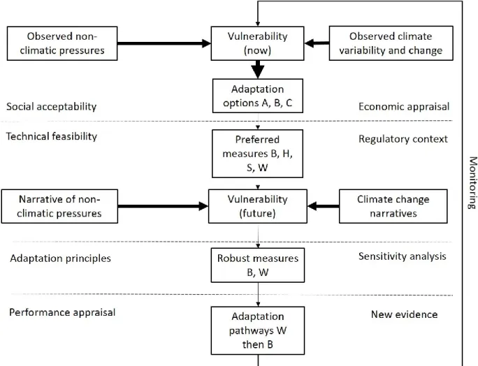
Figure 2-7: Conceptual framework used by Wilby and Dessai (2010) ... 40
Figure 2-8: Framework from Bhave et al. (2014) ... 41
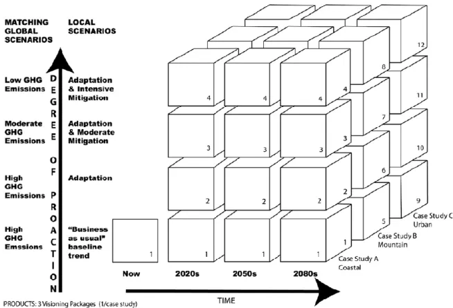
Figure 2-9: Future Visioning Process (Shaw et al., 2009; Sheppard et al., 2011) .... 42
Figure 2-10: The Decision Scaling Framework (Brown et al., 2012) ... 43
Figure 3-1: Location of the study area ... 46
Figure 3-2: Topography of the study area ... 47
Figure 3-3: Average monthly rainfall and evaporation (data source: IMHEN) ... 49
Figure 3-4: Uncertainties in a top-down approach (Wilby and Dessai, 2010) ... 55
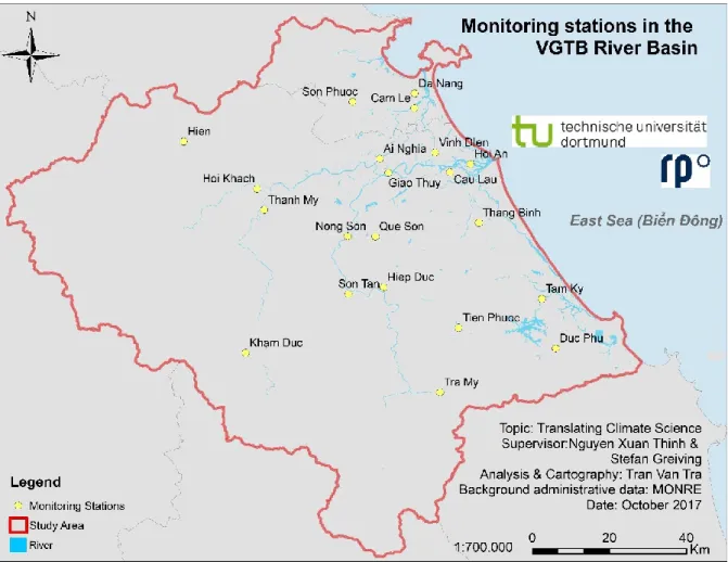
Figure 3-5: Monitoring stations in the Vu Gia- Thu Bon River Basin ... 57
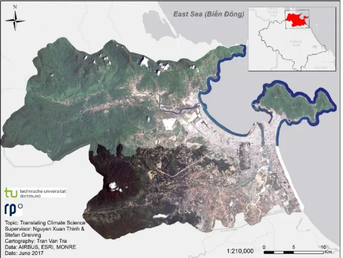
Figure 3-6: High Resolution SPOT image for Da Nang City ... 59
Figure 4-1: Overall Workflow of the research ... 62
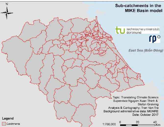
Figure 4-2: MIKE BASIN sub-basin delineation ... 65
Figure 4-3: MIKE NAM processes and parameters ... 66
Figure 4-4: Location of Nong Son and Thanh My catchments ... 70
Figure 4-5: Irrigation zones in the MIKE BASIN model ... 73
Figure 4-6: Schematic of important reservoir inputs ... 78
Figure 4-7: Visualization of bi-linear interpolation ... 81
Figure 4-8: Hierarchy classification scheme for land cover mapping ... 86
x
Figure 4-9: Confusion matrix post classification ... 87
Figure 4-10: Ground reference points for accuracy assessment ... 88
Figure 5-1: SWSI of 1998 in comparison with other drought years ... 93
Figure 5-2: Runoff at Nong Son gauge following the calibration process ... 94
Figure 5-3: Runoff at Nong Son gauge following the validation process ... 94
Figure 5-4: Runoff at Thanh My gauge following the calibration process ... 95
Figure 5-5: Runoff at Thanh My gauge following the validation process ... 95
Figure 5-6: MIKE BASIN model fully developed ... 102
Figure 5-7: Water supply reliability without upstream reservoirs (baseline period) 103 Figure 5-8: Water supply reliability with upstream reservoirs (baseline period) ... 104
Figure 5-9: Reliability of node IRR_VG07 ... 106
Figure 5-10: Reliability of node IRR_VG09 ... 106
Figure 5-11: Reliability of node IRR_VG12 ... 107
Figure 5-12: Reliability of node IRR_VG13 ... 108
Figure 5-13: Reliability of node IRR_TB09 ... 109
Figure 5-14: Reliability of node IRR_TB13 ... 109
Figure 5-15: Reliability of node IRR_TB15 ... 110
Figure 5-16: Reliability of node IRR_TB21 ... 111
Figure 5-17: Reliability of node IRR_VG23 ... 111
Figure 5-18: VGTB land cover in 2011 using supervised classification ... 118
Figure 5-19: VGTB land cover in 2016 using supervised classification ... 119
Figure 5-20: VGTB land cover in 2011 using index-based approach ... 120
Figure 5-21: VGTB land cover in 2016 using index based approach ... 121
Figure 5-22: Example of empty-land covered with vegetation ... 122
Figure 5-23: Comparison of Landsat 8 and SPOT 7 Images ... 124
Figure 5-24: Paddy rice area converted in between 2011 and 2016 ... 127
xi
Figure 5-25: Conversion of agricultural area into built-up area ... 128
Figure 5-26: Conversion of agricultural land into water bodies ... 131
Figure 5-27: Conversion of agricultural area into vegetation ... 132
Figure 5-28: Conversion of agricultural area into empty land ... 133
12
LIST OF TABLES
Table 3-1: Landsat satellite images used for the study ... 60
Table 4-1: Model parameters in MIKE NAM ... 66
Table 4-2: Weight of precipitation data used in Nong Son and Thanh My precipitation calculation... 70
Table 4-3: MIKE BASIN node corresponding to domestic water users ... 72
Table 4-4: Irrigation nodes with corresponding irrigation area, precipitation, and meteorological station data ... 76
Table 4-5: Land planning changes in Quang Nam and Da Nang until 2020 ... 83
Table 4-6: Description of land cover class classification ... 84
Table 5-1: Drought and water shortage years from literature ... 91
Table 5-2: SWSI value in year 1998 for Nong Son and Thanh My catchments ... 92
Table 5-3: MIKE NAM corresponding NASH-Sutcliffe value ... 96
Table 5-4: Calibrated MIKE NAM parameters ... 96
Table 5-5: Industrial water demand and corresponding node in MIKE BASIN ... 98
Table 5-6: Domestic water demand in the study area (calculated based on Vietnam Ministry of Construction (2006)) ... 99
Table 5-7: Domestic and industrial water demand (calculated based on Vietnam Ministry of Construction (2006)) ... 100
Table 5-8: Agricultural water demand under baseline condition (m3/s) ... 100
Table 5-9: Agricultural area at risks of water shortage ... 112
Table 5-10: Climate future for time period 2016-2035 (all scenarios) ... 113
Table 5-11: Climate future for time period 2046-2065 (all scenarios) ... 114
Table 5-12: Climate future for time period 2080-2099 (all scenarios) ... 114
Table 5-13: Maximum consensus case of GCM outputs... 116
Table 5-14: Best-case scenario of GCM outputs ... 116
13
Table 5-15: Worst-case scenario of GCM outputs ... 117
Table 5-16: Accuracy assessment of land cover classification using supervised classification ... 119
Table 5-17: Producer's and User's accuracy (supervised classification) ... 120
Table 5-18: Accuracy assessment of land cover classification using index based approach ... 121
Table 5-19: Producer's and User's accuracy of land cover classification (index method) ... 122
Table 5-20: Comparing land cover results with land use data from MONRE (units: km2) ... 123
Table 5-21: Land cover change matrix between 2011 and 2016 (units: km2) ... 125
Table 5-22: Land planning changes in Quang Nam and Da Nang until 2020 ... 126
Table 5-23: Conversion of agricultural land ... 128
Table 5-24: Average monthly income per capita in Quang Nam Province ... 129
Table 5-25: Population (inhabitants) and birth rate in the VGTB River Basin ... 130
Table 5-26: Gross output and contribution of agriculture and industry in the VGTB River Basin ... 130
14
LIST OF ABBREVIATIONS
CDO Climate Data Operators
CH4 Methane
CMPI5 Coupled Model Intercomparison Project Phase 5 CO2 Carbon Dioxide
DPSIR Driving forces, Pressures, States, Impacts, Responses DONRE Department of Natural Resources and Environment DEM Digital Elevation Model
DHI Danish Hydraulic Institute
GHG Greenhouse Gas
GIS Geographic Information System
GCM General Circulation Model/ Global Circulation Model LWR Long wave radiation
MONRE Ministry of Natural Resources and Environment
IMHEN Viet Nam Institute of Meteorology, Hydrology and Climate Change IPCC Intergovernmental Panel on Climate Change
NDBI Normalized Difference Built-up Index NDVI Normalized Difference Vegetation Index NDWI Normalized Difference Water Index NHMS National Hydro-Meteorological Service NO2 Nitrous dioxide
RCHM Regional Center for Hydrology and Meteorology RCM Regional Climate Model
RCP Representative Concentration Pathways SSP Shared Socioeconomic Pathways
SWR Short wave radiation
SWSI Surface Water Supply Index SO2 Sulfur Dioxide
UTM Universal Transverse Mercator VGTB Vu Gia- Thu Bon
15
1 INTRODUCTION
The motivation of the study is the realization that a traditional top-down climate change impact assessment have limitations in assisting adaptation policies both globally and in the VGTB River Basin. The first chapter of the report briefly states the problems related to climate change impact assessment and to illustrate the importance of a new approach. Research questions and research objectives are subsequently presented along with the structure of the report.
1.1 Background
Vu Gia- Thu Bon (VGTB) River Basin, located in the Central Coastal zone of Viet Nam, currently faces water shortages. Rainfall in the river basin is temporally variable with a distinct rainy season and a dry season. The rainy season, which begins in September and last until December, contributes approximately 70% to the total annual precipitation. On the other hand, the dry season spans the other 8 months within the year and contributes only 30% to total annual precipitation. Prolonged dry conditions with limited rainfall creates a huge challenge in water supply in the river basin.
As water resources will be the principal medium climate change impacts are felt (García, L.E. et al., 2014), the challenges of water management in the VGTB River Basin is likely to be exacerbated in the future. Temperature and rainfall changes could reduce water availability in the river basin. Increase temperature could lead to increase evapotranspiration and increase air moisture holding capacity, i.e. more water losses and less rain. On the other hand, decrease rainfall directly reduces runoff in the river basin. The effects could be seen in an overall drier condition with a reduction in water availability. Other extreme weather events such as droughts, and heat waves are then expected to increase in both frequency and intensity (García, L.E. et al., 2014; IPCC, 2012, 2013a).
There have been extensive studies into ways climate change impact the water systems in general and in the VGTB River Basin in particular. An increased understanding to recent date is the inertia of greenhouse gas (GHG) emissions in the past will likely accelerate climate change in the future. Hence, adaptation measures to climate change have gained increasing importance (Bhave et al., 2014). In order to
16
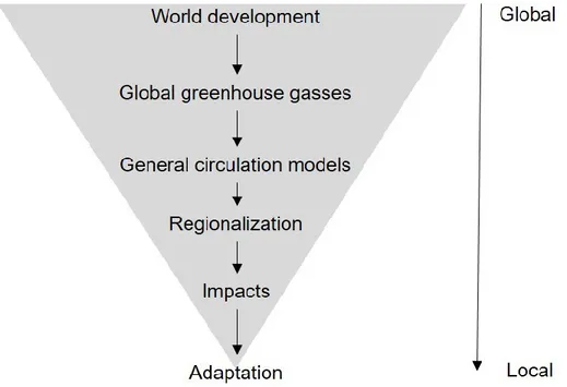
address the problem of climate change, traditionally a predict-then-act scheme is applied. Within this approach, future climate state is projected through downscaling outputs from climate models such as General Circulation Models (GCMs). The response of the system given the projected future climate state is consequently determined using hydrological models. The corresponding impacts to water resource are then evaluated and adaptation options determined (Brown et al., 2012).
And while this approach produce optimal results for the intended future, its usability remains relatively limited in terms of decision support and policy design due to the uncertainties of climate change (Stéphane Hallegatte et al., 2012; Brown et al., 2012).
Uncertainties in climate projection often come in the form of various climate change scenarios (e.g. RCPs) (IPCC, 2007a, 2013a) and socioeconomic scenarios (Shared Socioeconomic Pathways- SSP) (O’Neill et al., 2014; van Ruijven et al., 2014).
Variability from different projections can be large and to plan for one projection could strictly be contradictory to the other (Brown, 2011). Furthermore, the process of downscaling outputs from GCMs entails large uncertainties. This creates a gap in translating climate information into adaptation policy (Dilling and Lemos, 2011).
Additionally, the importance of land cover on water usage has been well established (Calijuri et al., 2015). Climate change affects the amount of water available while land cover change has an impact on the amount of water demanded. For this reason, there is also the need to provide land cover change information when addressing climate change impacts. This additional source of information would further benefit the adaptation process.
For the above mentioned reasons, this study seeks to adopt a different approach with less reliance on the use of GCMs and to omit the use of GCMs downscaling in climate change adaptation for the VGTB River Basin. Furthermore, the use of local information of land cover information is included. The result of the study includes better-tailored climate change information and providing policy makers with a list of proposed policies for climate change adaptation.
1.2 Research Questions and Objectives
The starting point that drives the motivation for the research is the knowledge that climate change will have an impact on the water system in the VGTB River Basin.
17
Although studies have focused on studying the impacts, a number of problem exists.
Firstly, the reliability of climate change impacts predictions in the VGTB River Basin has not been fully assessed. Projections and predictions into the future carry a certain level of uncertainty, yet this level of uncertainty has not been fully explored and communicated in previous researches. Secondly, there is a difference between the knowledge of climate change impacts and the response to these impacts in an active way. Since the reliability of the various predictions on climate change impacts in the VGTB has not yet been fully explored, would it be possible to propose adaptation measures in the light of this uncertainty?
1.2.1 Research questions
In this context, the main challenge of the research is the uncertainties related to climate change in the VGTB River Basin. A specific list of research questions were asked prior to conducting the research. These include:
1. What is the status of water shortage in the VGTB River Basin?
2. How will climate change impact rainfall and temperature in the VGTB River Basin?
3. How will the status of water shortage change in the future as climate changes?
4. How does land use policy affect water usage in the VGTB River Basin?
5. What are adaptation policies to climate change for the VGTB River Basin?
To be able to answer the aforementioned questions, it is desirable to set up a list of objectives of research in which key findings would provide information and addresses the motivation of research.
1.2.2 Research objectives
The overall objective of the research is to be able to translate climate change information into adaptation policies for the VGTB River Basin. As part of the process, the gap between the understanding of climate change impacts and the development of adaptation measures and strategies would need to be overcome.
Climate information may be readily available yet the information has to be made useful to decision makers. Scientific impact analysis and planning pursue different goals when put into the context of climate change. The former adopts reductionist approach to find evidence by considering the essence of a cause-and-effect chain, the latter
18
approach focuses on generating integrated solutions that cover all issues addressed.
Hence, a better method of translating and/or utilizing science of climate change to the understanding of policy/ decision makers that bridges the gap between producers and users of knowledge needs to be sought for.
Specific objectives in the pursuant of the overall objectives include:
1. To develop a hydrological model to further understand the response of the river basin in different climate states
2. To identify the range of possible changes in temperature and rainfall in the VGTB River Basin using GCMs and the response of the system to those changes
3. To determine the potential effects of land use policy in the VGTB River Basin 4. To be able to utilize the best available information on climate change in the
future to provide adaptation measures for policy makers
1.3 Structure of the Report
The report consists of 6 chapters. The first chapter introduces the topic and the structure of the report. Chapter 2 provides background theoretical basis that is useful in the study. Chapter 3 introduces the study area, the available data used in the study, and the justification for the study area selection. Chapter 4 introduces the methodology used. Chapter 5 discusses the results obtained and proposed adaptation measures based on the results. Chapter 6 provides conclusions and recommendations.
In chapter 2, conceptual basis in the context of climate change, hydrological modelling, and three climate change impact assessment approaches are provided.
The chapter covers concepts that would be required to understand the research gap provided in the subsequent chapter 3.
Chapter 3 provides a detailed introduction into the research area of VGTB River Basin. Justification of the study area selection is provided together with previous relevant researches. Through the identification of past research efforts, research gap was identified. This research gap provides the foundation of the research questions and research objectives.
19
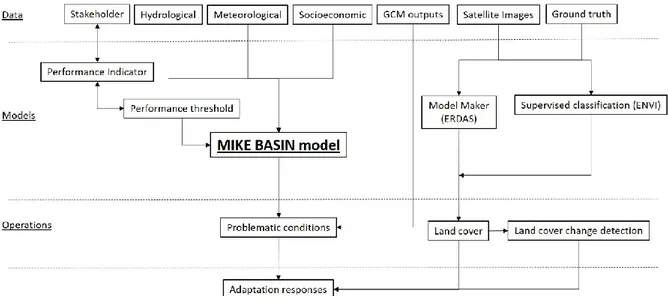
In order to fill the research gap, chapter 4 outlines the methods used in the study. The methodology consists of 5 parts. In the first part, the identification of climate hazards and threshold is described. This is performed using inputs from stakeholders and relevant experts, and analyzing the climate conditions of the VGTB River Basin. The second part describes the system model in use. In this case, the MIKE BASIN model is utilized. Various sub models are used namely the river basin model, the rainfall- runoff model, the water demand model, and the reservoir model. The fourth part establishes the method to discover climate risks. Climate variables, in particular temperature and precipitation are parametrically varied to simulate changing conditions in the river basin. Vulnerable climate space is then determined. In addition, output from General Circulation Models are utilized to map future temperature and precipitation conditions onto the vulnerability space identified earlier. The fourth component includes tailoring the information provided earlier to assist decision- making, i.e. combining the vulnerability space with possible future climate conditions in an easily understandable way. Lastly, the assessment of current land use policy is performed to provide further useful information for adaptation measures.
Chapter 5 presents and discusses the results obtained by using the methods proposed in chapter 4. The results are presented according to the components within chapter 4. Additionally, adaptation strategies are provided based on the results obtained from the analysis
Finally, chapter 6 refers back to the research objectives in chapter 1. Chapter 6 also discusses the shortcomings of the research and how this could be improved in the future. Other recommendations and future work are then presented.
21
2 THEORETICAL BASIS
Since the report deals with climate change impact assessment methods, this chapter provides an outline of the fundamental knowledge related to climate change. The cause of climate change and ways to predict climate change are further explained.
Water shortage in the context of climate change is also discussed. In addition, hydrological modelling is introduced as a tool to study the impacts of climate change on water systems.
2.1 Climate Change Background
Earth’s climate system has radically changed in the past. Over the last 700,000 years, glacial periods have occurred on average every 100,000 years due to the oscillation of both warmer and colder periods (García, L.E. et al., 2014). Historical records of changes in the past reveal the high sensitivity of the climate system to relatively small changes in the atmosphere. This includes heat retention and atmospheric circulation, such as a shift in the concentration of greenhouse gasses (GHG) both due to human- induced activities and natural sources (IPCC, 2013a).
Yet the topic of climate change is becoming more important in public policy agendas around the world in recent decades (Dilling and Lemos, 2011). One important aspect of climate change now is the speed of change has been accelerated by human activities through the increase of GHG in general and carbon dioxide in particular. The evidence of human influence on climate change has increased since the Fourth Assessment Report (IPCC, 2007b). In fact, it is now virtually certain that human influence has been the dominant cause of warming since the mid-20th century (IPCC, 2013a). Unprecedented levels of carbon dioxide (CO2), methane (CH4) and nitrous oxide (N2O) within the last 800,000 years have been reached. Levels of carbon dioxide in the atmosphere today as compared to levels before the industrial-time have increased by 40% (IPCC, 2013a).
2.1.1 Climate and weather
In discussing climate change, the distinction between climate and weather has to be made. Weather describes the atmospheric condition at a certain location and time
22
with indicators of temperature, pressure, humidity, wind and other parameters.
Weather also includes the presence of cloud, precipitation and phenomenon such as thunderstorms, dust storms, tornados and the like. Climate on the other hand describes the mean and variability of variables such as temperature, precipitation and wind over a longer period ranging from months to thousands and millions of years.
According to the World Meteorological Organization, a standard period of 30 years is used to determine the average value for climate (climate cycle). A broader definition of climate would further include associated statistics such as frequency, magnitude, persistence, trends (IPCC, 2013a).
Climate change, hence, refers to a change in the state of the climate that can be identified by changes in the mean and/or variability of its properties and that persists for an extended period. The key aspects of changes in mean and/or variability for an extended period of time is highly crucial. Without these two components, it is less likely to attribute changes to changes in climate but rather to the normal fluctuation of weather. Therefore, discussions of climate change have to bare this in mind.
2.1.2 Causes of climate change
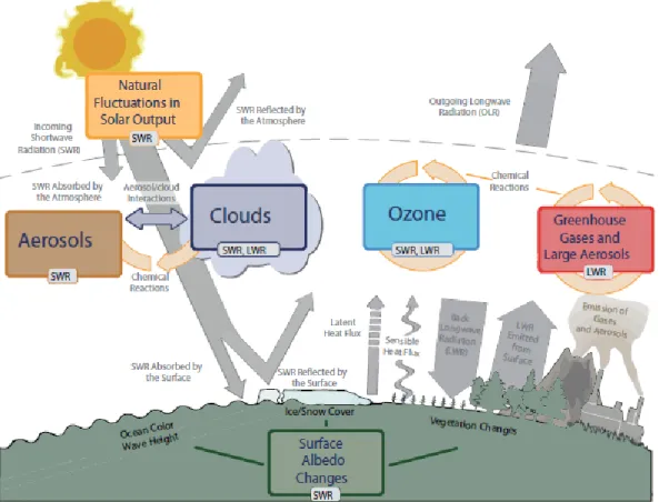
The Earth receives most of its energy from the Sun in the form of solar radiation. Solar radiation from the Sun, characterized by short wave length and high energy, drive the Earth’s climate system. Solar radiation provides heat to the Earth’s surface and atmosphere to sustain life. Roughly half of the solar radiation in the form of shortwave radiation (SWR) is absorbed by the Earth’s surface and stored as heat. The other half of SWR is either reflected back into space or absorbed by the atmosphere. The outgoing radiation from Earth in the form of longwave radiation (LWR, or infrared radiation) is mostly absorbed by certain atmospheric constituents such as water vapor (H2O), carbon dioxide (CO2), methane (CH4), nitrous oxide (N2O) and other gasses, which are categorized as greenhouse gasses (GHGs), and cloud in the atmosphere.
The downward directed component of the LWR adds heat to the lower layers of the atmosphere and to the Earth’s surface causing the greenhouse effect. The dominant energy loss of the infrared radiation from the Earth is from higher layers of the troposphere. The Sun provides its energy to the Earth primary in the tropics and subtropics; this energy is then partially redistributed to the middle and higher latitudes
23
by atmospheric and oceanic transport process. The overall process of incoming and outgoing radiation is depicted in Figure 2-1.
Figure 2-1: Main drivers of climate change (IPCC, 2007a)
As a result, changes in the global energy budget would come from either changes in the net incoming solar radiation or changes in the outgoing longwave radiation. Net incoming solar radiation changes comes from the changes in the Sun’s output energy or the Earth’s albedo. Changes in outgoing LWR can be a result of changes in the temperature of the Earth’s surface or atmosphere, or changes in the emission efficiency of LWR from either the atmosphere or the Earth’s surface. For the atmosphere, these changes in the emission efficiency are due predominantly to changes in cloud cover and cloud properties, GHGs and in aerosols concentrations.
The Earth’s energy budget is normally in equilibrium.
The influence of different aerosols on reflectivity of the Earth’s atmosphere can be highly variable. Some aerosols increase atmospheric reflectivity while others are strong absorbers and modify SWR. Aerosol can also indirectly affect cloud albedo since some aerosols serve as cloud condensation nuclei or ice nuclei. Therefore, changes in aerosol types and distribution in the atmosphere can ultimately lead to
24
changes in cloud albedo. Clouds play an important role in climate. Clouds can either increase albedo, thereby cooling the planet or increase warming through infrared radiative transfer. Depending on the physical properties of cloud such as level of occurrence, vertical extent, water path and effective cloud particle size, the net radiative effect of a cloud could be either cooling or warming. Human activities directly influence the greenhouse effect by emitting GHGs such as CO2, CH4, N2O and CFCs into the atmosphere. In addition, GHGs in the form of pollutants such as CO, volatile organic compounds (VOC), nitrogen oxides (NOx) and Sulphur dioxide (SO2) produced by human activities also have an indirect effect on the greenhouse effect by altering, through atmospheric chemical reactions, the abundance of important gases to the amount of outgoing LWR such as CH4 and ozone (O3), and/or by acting as precursors of secondary aerosols.
The impacts of human activities is not limited to changing atmospheric concentration of gasses and aerosols. Human activities further change land surface. Conversion of forest to cultivated land causes an imbalance in the energy and water budget of the planet through changing the characteristics of the vegetation, color, seasonal growth and carbon content. By clearing a forest for other use, carbon storage in vegetation is released back into the atmosphere. By clearing a vegetated land, the reflectivity of Earth’s surface, rates of evapotranspiration and long wave emissions changes.
The term radiative forcing (RF) refers to the measure of the net change in the energy balance in response to an external perturbation. The formation of radiative forcing is a direct result from changes in the atmosphere, land, ocean, biosphere and cryosphere both naturally and anthropogenically. These changes in the climate can include changes in the solar irradiance and changes in atmospheric trace gas and aerosol concentrations. However, the concept of RF does not include the interactions between anthropogenic aerosols and clouds. Therefore, to include the rapid response in the climate system, effective radiative forcing (ERF) is introduced. ERF is “the change in net downward flux at the top of the atmosphere after allowing for atmospheric temperatures, water vapor, clouds and land albedo to adjust, but with either sea surface temperature and sea ice cover unchanged of with global mean surface temperature unchanged” (IPCC, 2013a).
25
Once forcing is applied to the climate system, a system of complex feedback is triggered and determines the eventual response of the climate system. Feedback mechanisms in the climate system can be classified either as positive or negative. A positive feedback further amplifies the effects of the changes due to the forcing while a negative feedback has a diminishing effect. For example, an increase in surface temperature increases the amount of water vapor in the atmosphere; given that water vapor is an important GHG, an increase in water vapor would then further increases surface temperature and leads to further warming. Hence, surface temperature creates a positive feedback in reference to water vapor increase. Likewise, an increase in surface temperature or sea temperature causes ice caps to melt exposing darker and more absorbing surface beneath. While ice caps are more reflective surfaces, the removal of ice caps would then decrease the albedo leading to additional warming. Example of a negative feedback is the increased outgoing LWR as surface temperature increases (referred to as blackbody radiation feedback). It is important to note that the timescale in which different types of feedback operates can highly vary from hours through to decades and even centuries (IPCC, 2013a).
In short, the Earth has a natural mechanism of retaining energy and heat from solar radiation to support life. Since life on Earth is a highly dynamic system, the amount of energy and heat stored may fluctuate through time. However, given that the system on Earth is always in a dynamic equilibrium, the amount of energy and heat stored is also in a dynamic equilibrium. Human activities have released into the atmosphere an increased amount of GHG that increases the Earth’s ability to retain heat. A complex feedback system on Earth is then triggered leading to even further warming, causing the climate on Earth to change.
2.1.3 Climate Change Modeling and Projections
With the study of climate change, there are methods to predict the changes in climate variables such as temperature and rainfall due to changes in GHG concentrations and human activities. One approach that has been widely accepted in the past is the use of General Circulation Models (GCMs). This section introduces the core concept of GCMs and downscaling.
26 General circulation models
GCMs are numerical models that simulate the physical processes in the atmosphere, ocean, cryosphere and land surface in response to an increase in GHG emissions.
While there are a broad range of models which are also capable of determining the climate response, only GCMs have the potential to provide geographically and physically consistent estimates of regional climate change which are required in impact analysis (IPCC Data Distribution Center, 2013).
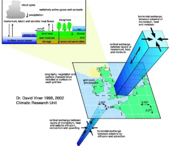
GCMs depict the climate using a three dimensional grid over the globe. A GCM typically has a horizontal resolution between 250km and 600km, 10 to 20 vertical layers in the atmosphere and sometimes as many as 30 layers in the oceans (IPCC Data Distribution Center, 2013). As a result, GCMs have relatively coarse resolution.
A schematic of a GCM grid is shown in Figure 2-2.
Figure 2-2: Schematic of a GCM grid (IPCC, 2013b)
Many physical processes, such as those related to clouds occur at smaller scales and cannot be properly modelled using GCMs. Instead, their known properties must be
27
averaged over the larger scale in a technique called parameterization. This is one source of uncertainty in GCM-based simulations of future climate.
Other uncertainties related to GCM simulations include the simulation of feedback mechanisms. For example, the uncertainties in modelling the feedback between water vapor and warming, clouds and radiation, ocean circulation and ice and snow albedo.
For this reason, GCMs may simulate different response to the same forcing, due to the way certain processes and feedbacks are modelled.
Downscaling
Despite the improvement of computing power in recent years, the horizontal resolution of GCMs are still too coarse to capture the effects of local climate change effects.
Most GCMs have resolutions up to a few hundred kilometers while climate change impacts are normally felt and dealt with at the more local and regional scale. For this reason, significant progress has been made in applying downscaling techniques to obtain local climate change projections at finer resolution, this includes dynamic downscaling through the use of regional climate model and statistical downscaling.
The use of Regional Climate Model (RCM) is one widely used method to add detail to climate projections. The use of regional climate model is sometimes referred to as
“dynamic downscaling” with a typical grid for climate change projection around 50 km, however, fine resolution up to 5km have been applied (IPCC, 2007a).
The regional climate model approach improves the resolution of climate projections through simulating at a sub GCM grid. In this approach, the RCM model is nested within the GCM grid and uses output from GCMs simulations to provide initial and driving lateral meteorological boundary conditions without accounting for the feedback from the RCM to the GCM. Therefore, the strategy in using RCM would be to first use the global model to simulate the response of global circulation to large scale forcing then use RCM to account for sub-GCM grid scale forcing and enhance the simulation of atmospheric circulations and climatic variables at fine spatial scales (IPCC, 2001).
Dynamic downscaling relies on driving Regional Climate Models (RCM) using outputs obtained from GCMs. RCM have higher spatial resolution and can then hence, represent climate variables at the local scale of interest (Tofiq and Guven, 2014).
Examples of highly successful researches in the past using the dynamical
28
downscaling approach includes Maraun et al. (2010); Xue et al. (2014) and Castro et al. (2005).
There are two main theoretical limitation of RCMs including the effects of systematic errors in the driving fields provided by the global model and the lack of two-way interaction between regional and global climate. RCMs can also be computational demanding depending on the domain size and resolution hence limiting the ability to perform multi-model run. And finally, the temporal frequency of GCM fields (6 hours or higher) can mismatch that required by RCM, hence, careful consideration is needed when nesting RCM into GCM grids (IPCC, 2001).
Another approach in downscaling GCMs is through statistical downscaling. Statistical downscaling is based on the view that regional climate is influenced by large-scale climatic states and regional/local physiographic features (topography, land use, etc.).
From this view point, statistical downscaling is mainly a two-step process including firstly develop a meaningful statistical relationship between climate variables at the local scale and the large scale predictors and then applying such a relationship to the output of GCM models to simulate local climate characteristics (IPCC, 2001).
The statistical downscaling approach seeks to establish a statistical relationship between large-scale variables such as atmospheric pressures and a local variable such as wind speed at a particular site of interest. Statistical downscaling facilitates the rapid development of multiple, low cost, single-site scenarios of daily surface water variables under current and future regional climate forcing (Tofiq and Guven, 2014). A number of studies were also successfully conducted by using statistical downscaling and different GCM scenarios to predict the runoff based on precipitation and rainfall-runoff models (Yonggang et al., 2013; Chen et al., 2012; Scmidli et al., 2007).
A statistical downscaling approach has both advantages and disadvantages. The main advantage of a statistical downscaling method is computational efficiency. Since the majority of statistical downscaling model are able to produce results faster than regional climate models, a range of output from different GCM models could potentially be applied instead of using just one projection. The main disadvantage of a statistical downscaling method lies in the fundamental viewpoint of the method. In other words, a relationship between large-scale climatic state and regional
29
physiographic feature does not necessarily hold true in the future under different forcing conditions.
2.2 Water Shortages and Climate Change
Climate change in both the context of natural variability and due to human activities can lead to changes in extreme weather and climate events. Extreme precipitation events leading to severe flooding or extreme dry spells leading to drought conditions can be excellent examples. By definition, an extreme weather event is “one that is rare at a particular place and/or time of the year” (IPCC, 2013a). Due to the misconception of weather and climate, there can be false classification of extreme events. At present, single extreme event is unlikely to be attributed to anthropogenic influence. Only when a pattern of extreme weather persists for at least some time, for instance a season or several months, then the event itself can be identified as an extreme event. For example, drought or heavy rainfall over a season long. Important factors contributing to an extreme event includes duration and intensity, especially in the case of drought and water shortage (IPCC, 2012).
In the context of climate change, there still exist high uncertainties in observing trends of drought on a global scale (IPCC, 2012). Evidence summarized in the Fourth Assessment Report (AR4) of the Intergovernmental Panel on Climate Change have shown that very dry areas have more than doubled in extent since 1970 globally. The assessment was made using the Palmer Drought Severity Index and based largely on the study by Dai et al. (2004). The results showed high sensitivity to changes in temperature rather than precipitation (IPCC, 2012).
Another study simulating soil moisture with an observation land surface model by Sheffield and Wood (2008) have determined that the trends in drought duration, intensity and severity being predominantly decreasing worldwide in the time period between 1950-2000. However, the study provided strong regional variation including strong increases in some regions. The study then concluded that the overall trend is moistening over the considered period with a switch starting from the 1970s to a drying trend, especially in the high northern latitudes.
Other regional studies have also arrive at a similar result that are consistent with the conclusion from Sheffield and Wood (2008), i.e. there is no widespread increase in
30
drought trends globally as stated by Dai et al. (2004). A more recent study by Dai (2011) extended the record and found a widespread in drought based on PDSI values for the time period of 1950-2008 and output from soil moisture land surface model for the period of 1948-2004. For this reason, there are still large uncertainties in assessing global drought trends.
However, from the range of evidence, the AR4 concluded that it is more likely than not the increase of drought in the late 20th century is partially or substantially due to anthropogenic activities. Instrumental observations over the past 157 years show that temperature at the surface has risen globally. The increase is highly variable from region to region, yet globally occurred in two phases beginning from 1910 to the 1940s (Mishra and Singh, 2010). Consequently, drought extremes could also be expected to increase within the line of temperature. Additionally, a detection study identifying anthropogenic fingerprint in a global PDSI data set showed high significance (IPCC, 2012).
The more recent Fifth Assessment Report (AR5) agreed with AR4 that anthropogenic influence has contributed to the increased risk of drought in the second half of the 20th century. However, AR5 no longer supports the claim of increasing hydrological drought trends since the 1970s supported by AR4. In addition, due to the low confidence in observed large scale trends in dryness and variability of drought, there is now low confidence in the attribution of changes in drought over global land since the mid-20th century to human influence (IPCC, 2013a).
Given the range of different results, it can be seen that uncertainty exists on the overall water shortage and drought conditions due to climate change globally. Nonetheless, it has now been commonly accepted that droughts in the future pose a serious threat to human systems, especially in the case of agricultural production. Therefore, there is a large research demand into the possible impact of droughts and water shortage in the future to assist developing adaptation measures.
2.3 Hydrologic modeling
To assess the extent of water shortages in reality, different methods have been applied. This includes the use of hydrologic models. The objective of these models is to simulate the relationship between various variable within a river basin to produce
31
outputs such as river flow from rainfall. Many of these models utilize advanced mathematical techniques and attempt to mimic the natural processes that occur within a basin level. However, there is still no consensus about the processes that occur in the natural system, therefore, this uncertainty has been represented by a many number of different models.
Three modeling approaches have generally been used in the development of hydrologic modeling. This includes a data-driven, a process-driven, and a conceptual model.
2.3.1 Process- driven modelling
Process-driven modeling is based on an understanding of the individual processes that occur within a basin. While in theory, the ability to use the processes to obtain outputs such as river flow and water level from rainfall should result in a wide range of applicability, this has not been the case in practice. This is because not all of the relevant processes that occur are fully understood, and some of the processes are not able to be represented mathematically. As Blöschl, G. and Sivapalan M. (1995) suggested, processes that are important at one scale may be irrelevant at another scale. Thus, the complexity embedded within a process-driven model may be superfluous. As a result, process-driven models often contain an excessive number of parameters. Consequently, an extensive amount of data is required in the development of process-driven models (Sivapalan, 2003).
2.3.2 Data- driven modelling
Data-driven modeling is concerned with the overall behavior of the system at a larger scale (Littlewood et al., 2003). The selection and interaction of the relevant components of the model are dependent on an analysis of data obtained from the catchment, rather than from the processes that occur (Sivapalan, 2003). These data- driven models have been used with moderate success in predicting rainfall-runoff behavior (Chiew, F.H.S and Siriwardena, L., 2005). More importantly, data-driven models do not usually require as much data to develop as process-driven models, and are typically parametrically parsimonious (Littlewood et al., 2003). In other words, they use fewer parameters without a loss in accuracy.
32
2.3.3 Conceptual hydrological models
In practice, the extreme idealized states of either data-driven or process-driven models are not often used, and an assimilation of the two approaches is adopted.
This is mainly because process-driven models have to use data-driven procedures to establish the plausibility of the physical processes that occur. On the other hand, most data-driven models assume a form of underlying relationship which is the principle underlying process-driven models. Therefore, a combination of the two is usually used instead. These combination models based on both data-driven and process-driven models are termed conceptual models.
While the equations and the solution procedures may vary depending on the model used, all hydrological models have the following common components (US Army Corps of Engineers, 2000):
State variables represent the state of a system at a particular time and location.
Parameters which are numerical measures of the properties of the real world system. They control the relationship of the system input to system output.
Parameters can have physical significance or may be purely empirical.
Boundary conditions of the system input which forces the system to change
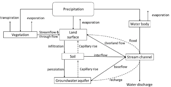
Initial conditions which are values of the output given before computation Conceptual hydrological models describe how a basin responds to a precipitation event and flows of water from upper stream. The general hydrologic processes represented by models is shown in Figure 2-3. The processes illustrated begin with precipitation. In the simple conceptualization shown, the precipitation can fall on the watershed’s vegetation, land surface, and water bodies (streams and lakes).
33
Figure 2-3: Runoff processes (US Army Corps of Engineers, 2000)
In the natural hydrologic system, much of the precipitation water returns to the atmosphere in the form of evaporation from vegetation, land surfaces, and water bodies and through transpiration from vegetation. During a storm, the amount of evaporation and transpiration is small.
Further precipitation on vegetation could avoid interception and fall through the leaves or run down stems, branches and trunks and reach land surface. At the land surface, water may pond, and depending on the soil type, ground cover, antecedent soil moisture and other watershed properties, a portion may infiltrate. This infiltrated water is stored temporarily in the upper, partially saturated layers of soil. From there, it rises to the surface again by capillary action, moves horizontally as interflow just beneath the surface, or it percolates vertically to the groundwater aquifer. The interflow eventually moves into the stream channel. Water in the aquifer moves slowly, but eventually, some returns to the channels as baseflow.
Water that does not pond or infiltrate moves by overland flow to a stream channel.
The stream channel is the combination point for the overland flow, the precipitation that falls directly on water bodies in the watershed, and the interflow and baseflow.
Thus, resultant streamflow is the total watershed outflow.
Conceptual hydrologic models mimics this natural cycle and to an extent simplify these processes into mathematical formulations. Hydrologic models could further incorporate other components of the hydrologic system that are beyond the natural