Towards Adjusting Mobile Devices To User's Behaviour

Towards Adjusting Mobile Devices to User’s Behaviour

Peter Fricke

, Felix Jungermann

, Katharina Morik

, Nico Piatkowski

, Olaf Spinczyk

, Marco Stolpe

, and Jochen Streicher

1

Technical University of Dortmund, Artificial Intelligence Group Baroper Strasse 301, Dortmund, Germany

{fricke,jungermann,morik,piatkowski,stolpe}@ls8.cs.tu-dortmund.de, http://www-ai.cs.tu-dortmund.de

2

Technical University of Dortmund, Embedded System Software Group Otto-Hahn-Strasse 16, Dortmund, Germany {olaf.spinczyk,jochen.streicher}@tu-dortmund.de,

http://ess.cs.uni-dortmund.de

Abstract. Mobile devices are a special class of resource-constrained em- bedded devices. Computing power, memory, the available energy, and network bandwidth are often severely limited. These constrained re- sources require extensive optimization of a mobile system compared to larger systems. Any needless operation has to be avoided. Time- consuming operations have to be started early on. For instance, load- ing files ideally starts before the user wants to access the file. So-called prefetching strategies optimize system’s operation. Our goal is to ad- just such strategies on the basis of logged system data. Optimization is then achieved by predicting an application’s behavior based on facts learned from earlier runs on the same system. In this paper, we ana- lyze system-calls on operating system level and compare two paradigms, namely server-based and device-based learning. The results could be used to optimize the runtime behaviour of mobile devices.

Keywords: Mining system calls, ubiquitous knowledge discovery

1 Introduction

Users demand mobile devices to have long battery life, short application startup

time, and low latencies. Mobile devices are constrained in computing power,

memory, energy, and network connectivity. This conflict between user expecta-

tions and resource constraints can be reduced, if we tailor a mobile device such

that it uses its capacities carefully for exactly the user’s needs, i.e., the services,

that the user wants to use. Predicting the user’s behavior given previous be-

havior is a machine learning task. For example, based on the learning of most

often used file path components, a system may avoid unnecessary probing of files and could intelligently prefetch files. Prefetching those files, which soon will be accessed by the system, leads to a grouping of multiple scattered I/O requests to a batched one and, accordingly, conservation of energy.

The resource restrictions of mobile devices motivate the application of ma- chine learning for predicting user behavior. At the same time, machine learning dissipates resources. There are four critical resource constraints:

– Data gathering: logging user actions uses processing capacity.

– Data storage: the training and test data as well as the learned model use memory.

– Communication: if training and testing is performed on a central server, sending data and the resulting model uses the communication network.

– Response time: the prediction of usage, i.e., the model application, has to happen in short real-time.

The dilemma of saving resources at the device through learning which, in turn, uses up resources, can be solved in several ways. Here, we set aside the prob- lem of data gathering and its prerequisites on behalf of operation systems for embedded systems [15] [24] [3]. This is an important issue in its own right. Re- garding the other restrictions, especially the restriction of memory, leads us to two alternatives.

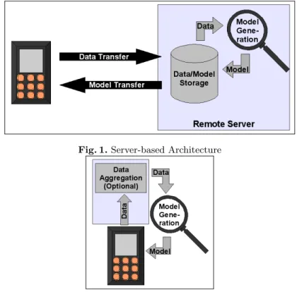
Server-based learning: The learning of usage profiles from data is performed on a server and only the resulting model is communicated back to the de- vice. Learning is less restricted in runtime and memory consumption. Just the learned model must obey the runtime and communication restrictions.

Hence, a complex learning method is applicable. Figure 1 shows this alter- native.

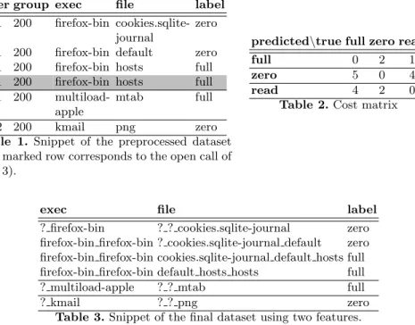
Device-based learning: The learning of usage profiles on the device is severely restricted in complexity. It does not need any communication but requires training data to be stored. Data streaming algorithms come into play in two alternative ways. First, descriptive algorithms incrementally build-up a com- pact way to store data. They do not classify or predict anything. Hence, in addition, simple methods are needed that learn from the aggregated compact data. Second, simple online algorithms predict usage behavior in realtime.

The latter option might only be possible if specialized hardware is used, e.g., General Purpose GPUs. Figure 2 shows this alternative.

In this paper, we want to investigate the two alternatives using logged sys-

tem calls. Server-based learning is exemplified by predicting file-access patterns

in order to enhance prefetching. It is an open question whether structural models

are demanded for the prediction of user behavior on the basis of system calls,

or simpler models such as Naive Bayes suffice. Should the sequential nature of

system calls be taken into account by the algorithm? Or is it sufficient to en-

code the sequences into the features? Or should features as well as algorithm be

capable of explicitly utilizing sequences? In order to address these questions, we

Fig. 1. Server-based Architecture

Fig. 2. Device-based Architecture

investigate the use of two extremes: Conditional Random Fields (CRF) – which use sequential information – and Naive Bayes (NB) – which ignores sequential dependencies among the labels. In particular, we inspect their memory consump- tion and runtime, both, for training and applying the learned function. Section 2 presents the study of server-based learning for ubiquitous devices. We derive the learning task from the need of enhancing prefetching strategies, describe the log data used, and present the learning results together with resource consumptions of NB and CRF.

Device-based learning is exemplified by recognizing applications from system

calls in order to prevent fraud. We apply the data streaming algorithm Hierar-

chical Heavy Hitters (HHH) yielding a compact data structure for storage. Using

these, the simple kNN method classifies systems calls. In particular, we investi-

gate how much HHH compress data. Section 3 presents the study of device-based

learning using a streaming algorithm for storing compact data. We conclude in

Section 4 by indicating related and future work.

2 Server-based Learning

We present the first case-study, where log data is stored and analyzed on a server. The acquisition is described in Section 2.2 and the data itself in Section 2.3. Learning aims at predicting file access in order to prefetch files (see Section 2.1). The learning methods NB and CRF are introduced shortly in Section 2.4 and Section 2.5, respectively. The results are shown in Section 2.6.

2.1 File-access pattern prediction

A prediction of file-access patterns is of major importance for the performance and resource consumption of system software. For example, the Linux operating system uses a large “buffer cache” memory for disk blocks. If a requested disk block is already stored in the cache (cache hit ), the operating system can deliver it to the application much faster and with less energy consumption than oth- erwise (cache miss). In order to manage the cache the operating system has to implement two strategies, block replacement and prefetching. The block replace- ment strategy is consulted upon a cache miss: a new block has to be inserted into the cache. If the cache is already full, the strategy has to decide which block has to be replaced. The most effective victim is the one with the longest forward distance, i.e. the block with the maximum difference between now and the time of the next access. This requires to know or guess the future sequence of cache access. The prefetching strategy proactively loads blocks from disk into the cache, even if they have not been requested by an application, yet. This of- ten pays off, because reading a bigger amount of blocks at once is more efficient than multiple read operations. However, prefetching should only be performed if a block will be needed in the near future. For both strategies, block replacement and prefetching, a good prediction of future application behavior is crucial.

Linux and other operating systems still use simple heuristic implementations of the buffer cache management strategies. For instance, the prefetching code in Linux [2] continuously monitors read operations. As long as a file is accessed sequentially the read ahead is increased. Certain upper and lower bounds restrict the risk of mispredictions. This heuristics has two flaws:

– No prefetching is performed before the first read operation on a specific file, e.g., after “open”, or even earlier.

– The strategy is based on assumptions on typical disk performance and buffer cache sizes, in general. However, these assumptions might turn out to be wrong in certain application areas or for certain users.

Prefetching based on machine learning avoids both problems. Prefetching can

already be performed when a file is opened. It only depends on the prediction

that the file will be read. The prediction is based on empirical data and not on

mere assumptions. If the usage data change, the model changes, as well.

2.2 System Call Data Acquisition

Logging system calls in the Linux kernel does not only require instrumentation, but also a mechanism to transport the collected data out of the kernel space.

Since the kernel’s own memory pages cannot be swapped out of the main mem- ory, kernel memory is usually kept as small as possible. Therefore, data transport has to happen frequently and should thus be efficient.

A convenient tool for this purpose is SystemTap [8], which allows the use of an event-action language for kernel instrumentation. The most important language element is the probe, which consists of two parts: The first part describes events of interest, like system calls, in a declarative manner. The second part is a corresponding handler, which is written in a C-like typesafe language. When at least one of the specified events of a probe occurs, the handler is executed.

The handlers usually write collected data into an in-kernel buffer, but they may also preprocess or accumulate data first. Depending on the type of an event, the handler has access to context information, like function parameters and return values. Global kernel data, like the current thread ID, is always accessible.

SystemTap provides a compiler, which translates the probe definitions into a loadable kernel extension module. As soon as the module is loaded, it instruments all associated points in the kernel machine code with calls to corresponding probe handlers. After that, Systemtap’s runtime system constantly moves the generated data from kernel to user space.

Data Acquisition on Android-based Devices Our mobile system call data source was an HTC Desire smartphone, which is based on the mobile operating system Android.

Although Android has a Java-based application layer, the layers below con- tain all essential parts of an embedded Linux system. Besides the kernel itself, there are also all standard libraries and tools that are required to run SystemTap.

However, the kernel included in a device vendor’s standard installation usually has several features disabled that are essential for using SystemTap, e.g., support for instrumentation.

To build a SystemTap-enabled kernel, we used Cyanogenmod

, an Android- based software distribution, which exists in various device-specifically customized variants. The original Android sources contain only a generic Linux kernel, which does not necessarily support all the hardware components of a specific device.

SystemTap’s workflow for embedded devices is designed to perform as much work as possible on an external, more powerful machine (the host), leaving only necessary parts on the mobile device (the target). The probe definitions are compiled on the host, which contains most of the SystemTap software, as well as the debug information for the target’s kernel. The target contains merely the runtime and, of course, the compiled instrumentation modules.

3

We used Cyanogenmod 7.0.0, which is based on Android 2.3.3. The kernel release was

2.6.32.28. Cyanogenmod can be downloaded from http://www.cyanogenmod.com/

The average amount of log data per day was only 11 MiB in size. Thus, we could store the entire log file on the device’s internal flash drive. In order to preserve the user’s privacy, it is planned to encrypt the log data in future experiments. The instrumentation did not have any user-observable impact on performance and responsiveness during typical operation (e.g., phoning, writing text messages, playing audio files, and browsing the web).

2.3 System Call Data for Access Prediction

We logged streams of system calls of type FILE on a desktop system as well as an Android-based mobile phone. System calls consist of various typical sub- sequences, each starting with an open- and terminating with a close-call, like those shown in Figure 3 and 4. We collapsed such sub-sequences to one obser- vation and assign the class label

– full, if the opened file was read from the first seek (if any) to the end, – read, if the opened file was randomly accessed and

– zero, if the opened file was not read after all.

1,open,1812,179,178,201,200,firefox,/etc/hosts,524288,438,7 : 361, full 2,read,1812,179,178,201,200,firefox,/etc/hosts,4096,361

3,read,1812,179,178,201,200,firefox,/etc/hosts,4096,0 4,close,1812,179,178,201,200,firefox,/etc/hosts

Fig. 3. A sequence of system calls to read a file. The data layout is: timestamp, syscall, thread-id, process-id, parent, user, group, exec, file, parameters (optional) : read bytes, label (optional)

1,open,14,14,1,25,100,gconfd-2,/path/to/gconf.xml.new,65,384,47 : 0, zero 2,llseek,14,14,1,25,100,gconfd-2,/path/to/gconf.xml.new,1,0,96

3,write,14,14,1,25,100,gconfd-2,/path/to/gconf.xml.new,697 4,close,14,14,1,25,100,gconfd-2,47

Fig. 4. A sequence of system calls to write some blocks to a file. The data layout is the same as for Figure 3.

We propose the following generalization of obtained filenames. If a file is regular, we remove anything except the filename extension. Directory names are replaced by ”DIR”, except for paths starting with ”/tmp” – those are replaced by

”TEMP”. Any other filenames are replaced by ”OTHER”. This generalization of

filenames yields good results in our experiments. Volatile information like thread- id, process-id, parent-id and system-call parameters is dropped, and consecutive observations are compound to one sequence if they belong to the same process.

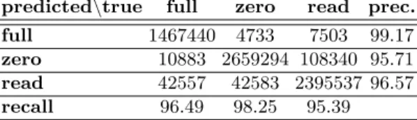
The resulting dataset consists of 673887 observations for the desktop log data and 18257 for the Android log data. These are aggregated into 80661 and 3328 sequences, respectively. A snippet

is shown in Table 1.

user group exec file label 201 200 firefox-bin cookies.sqlite-

journal

zero 201 200 firefox-bin default zero 201 200 firefox-bin hosts full 201 200 firefox-bin hosts full 201 200 multiload-

apple

mtab full

102 200 kmail png zero

Table 1. Snippet of the preprocessed dataset (the marked row corresponds to the open call of Fig. 3).

predicted\true full zero read

full 0 2 1

zero 5 0 4

read 4 2 0

Table 2. Cost matrix

exec file label

? firefox-bin ? ? cookies.sqlite-journal zero firefox-bin firefox-bin ? cookies.sqlite-journal default zero firefox-bin firefox-bin cookies.sqlite-journal default hosts full firefox-bin firefox-bin default hosts hosts full

? multiload-apple ? ? mtab full

? kmail ? ? png zero

Table 3. Snippet of the final dataset using two features.

We used two feature sets for the given task. The first encodes information about sequencing as features, resulting in 24 features, namely f

, f

, f

, f

/f

, f

/f

, f

/f

/f

, with f ∈ {user, group, exec, f ile}. The second feature set simply uses two features exec

/exec

and f ile

/f ile

/f ile

as its only features – an excerpt of the dataset using these two features is shown in Table 3.

Errors in predicting the types of access result in different degrees of fail- ure. Predicting a partial caching of a file, if just the rights of a file have to be changed, is not as problematic as predicting a partial read if the file is to be read completely. Hence, we define a cost-matrix (see Table 2) for the evaluation of our approach. For further research the values used in this matrix might have

4

The final dataset is available at:

http://www-ai.cs.tu-dortmund.de/PUBDOWNLOAD/MUSE2010

to be readjusted based on results of concrete experiments on mobile devices or simulators.

2.4 Naive Bayes Classifier

The Naive Bayes classifier (cf. [11]) assigns labels y ∈ Y to examples x ∈ X . Each example is a vector of m attributes written here as x

, where i = 1...m.

The probability of a label given an example is according to the Bayes Theorem:

p(Y |x

, x

, ..., x

) = p(Y )p (x

, x

, ..., x

|Y )

p (x

, x

, ..., x

) (1) Domingos and Pazzani [7] rewrite eq. (1) and define the Simple Bayes Classifier (SBC):

p(Y |x

, x

, ..., x

) = p(Y ) p (x

, x

, ..., x

)

n

Y

j=1

p (x

|Y ) (2)

The classifier delivers the most probable class Y for a given example x = x

. . . x

:

arg max

Y

p(Y |x

, x

, ..., x

) = p(Y ) p (x

, x

, ..., x

)

m

Y

j=1

p (x

|Y ) (3)

The term p (x

, x

, ..., x

) can be neglected in eq. (3) because it is a constant for every class y ∈ Y . The decision for the most probable class y for a given example x just depends on p(Y ) and p (x

|Y ) for i = 1 . . . m. These probabilities can be calculated after one run on the training data. So, the training runtime is O(n), where n is the number of examples in the training set. The number of probabilities to be stored during training are |Y| + ( P

i=1

|X

| ∗ |Y|), where

|Y| is the number of classes and |X

| is the number of different values of the ith attribute. The storage requirements for the trained model are O(mn).

It has often been shown that SBC or NBC perform quite well for many data mining tasks [7, 12, 9].

2.5 Linear-chain Conditional Random Fields

Linear-chain Conditional Random Fields, introduced by Lafferty et al. [14], can be understood as discriminative, sequential version of Naive Bayes Classifiers.

The conditional probability for an actual sequence of labels y

, y

, ..., y

, given a

sequence of observations x

, x

, ..., x

is modeled as an exponential family. The

underlying assumption is that a class label at the current timestep t just depends

on the label of its direct ancestor, given the observation sequence. Dependency

among the observations is not explicitly represented, which allows the use of

rich, overlapping features. Equation 4 shows the model formulation of linear- chain CRF

p

(Y = y|X = x) = 1 Z (x)

T

Y

t=1

exp X

k

λ

f

(y

, y

, x)

!

(4)

with the observation-sequence dependent normalization factor

Z (x) = X

y T

Y

t=1

exp X

k

λ

f

(y

, y

, x)

!

(5)

The sufficient statistics or feature functions f

are most often binary indicator functions which evaluate to 1 only for a single combination of class label(s) and attribute value. The parameters λ

can be regarded as weights or scores for this feature functions. In linear-chain CRF, each attribute value usually gets |Y|+|Y|

parameters, that is one score per state-attribute pair as well as one score for ev- ery transition-attribute triple, which results in a total of P

i=1

|X

| |Y| + |Y|

model parameters, where |Y| is the number of classes, m is the number of at- tributes and |X

| is the number of different values of the ith attribute. Notice that the feature functions explicitly depend on the whole observation-sequence rather than on the attributes at time t. Hence, it is possible and common to involve attributes of preceding as well as following observations from the current sequence into the computation of the total score exp ( P

k

λ

f

(y

, y

, x)) for the transition from y

to y

given x.

The parameters are usually estimated by the maximum-likelihood method, i.e., maximizing the conditional likelihood (Eq. 6) by quasi-Newton [16], [21], [17] or stochastic gradient methods [27], [19], [20].

L (λ) =

N

Y

i=1

p

(Y = y

|X = x

) (6)

The actual class prediction for an unlabeled observation-sequence is done by the Viterbi algorithm known from Hidden Markov Models [23], [18].

Although CRF in general allow to model arbitrary dependencies between the class labels, efficient exact inference can solely be done for linear-chain CRF.

This is no problem here, because they match the sequential structure of our system-call data, presented in section 2.3.

2.6 Results of Server-based Prediction

Tables 4 to 9 are showing the results on the desktop dataset and Tables 10

to 15 for Android, respectively. Comparing the prediction quality of the simple

NB models and the more complex CRF models, surprisingly, the CRF are only

slightly better when using the two best features. CRF outperforms NB when

using all features. These two findings indicate that the sequence information is

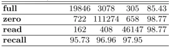
not as important as we expected. Neither encoding the sequence into features nor applying an algorithm which is made for sequential information outperforms a simple model. The Tables show that precision, recall, accuracy, and misclas- sification cost are quite homogeneous for CRF, but vary for NB. In particular, the precision of predicting “read” and the recall of class “zero” differs from the numbers for the other classes, respectively. This makes CRF more reliable. The results on the Android log data resemble those on the desktop log except for the precision on label ”full”. This might be caused by the lower number of recorded system calls as well as different label proportions.

Inspecting resource consumption, we stored models of the two methods for both feature sets and for various numbers of examples to show the practical storage needs of the methods. Table 16 presents the model sizes of the naive Bayes classifier on both feature sets and for various example set sizes. We used the popular open source data mining tool RapidMiner

for these experiments.

Table 16 also shows the model sizes of CRF on both feature sets and various example set sizes.

We used the open source CRF implementation CRF++

with L

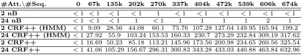
-regularization, σ = 1 and L-BFGS optimizer in all CRF experiments. Obviously, the storage needs for a model produced by a NB classifier are lower than those for a CRF model. This is the price to be paid for more reliable prediction quality. CRF don’t scale-up well. Considering training time, the picture becomes worse. Table 17 shows the training time of linear-chain or HMM-like CRF consuming orders of magnitude more time than NB.

3 Device-based Learning

In this section, we present the second case-study, where streams of log data are processed in order to store patterns of system use. The goal is to aggregate the streaming system data. A simple learning method might then use the aggregated data. The method of Hierarchical Heavy Hitters (HHH) is defined in Section 3.1.

The log data are shown in Section 3.2. For the comparison of different sets of HHH, we present a distance measure that allows for clustering or classifying sets of HHH. In addition to the quality of our HHH application, its resource consumption is presented in Section 3.3.

3.1 Hierarchical Heavy Hitters

The heavy hitter problem consists of finding all frequent elements and their fre- quency values in a data set. According to Cormode [4], given a (multi)set S of size N and a threshold 0 < φ < 1, an element e is a heavy hitter if its fre- quency f (e) in S is not smaller than bφNc. The set of heavy hitters is then HH = {e|f (e) ≥ bφN c}.

5

RapidMiner is available at: http://www.rapidminer.com

6

CRF++ is available at: http://crfpp.sourceforge.net/

predicted\true full zero read prec.

full 1427467 19409 3427 98.43

zero 12541 2469821 40258 97.91 read 80872 217380 2467695 89.22 recall 93.86 91.25 98.26

Table 4. Result of Naive Bayes Classifier on the best two features, 10x10-fold cross-validated, accu- racy: 94.45 ± 0.0, missclassification costs: 0.152 ± 0.01

full zero read prec.

1426858 21562 22717 96.99 15392 2371009 97566 95.45 78630 314039 2391097 85.89 93.82 87.60 95.21

Table 5. Result of Naive Bayes Classifier on all 24 features, 10x10-fold cross-validated, accu- racy: 91.84 ± 0.0, missclassifica- tion costs: 0.218 ± 0.02

predicted\true full zero read prec.

full 1446242 7123 29051 97.56

zero 19452 2639097 133007 94.54 read 55186 60390 2349322 95.31 recall 95.09 97.51 93.55

Table 6. Result of HMM-like CRF on the best two features, 10x10-fold cross-validated, accuracy:

95.49 ± 0.0, missclassification costs: 0.150 ± 0.0

full zero read prec.

1450147 8335 25629 97.71 14563 2639724 126403 94.93 56170 58551 2359348 95.36 95.35 97.53 93.95

Table 7. Result of HMM-like CRF on all 24 features, 10x10-fold cross-validated, accuracy: 95.70 ± 0.0, missclassification costs: 0.143

± 0.0 predicted\true full zero read prec.

full 1467440 4733 7503 99.17

zero 10883 2659294 108340 95.71 read 42557 42583 2395537 96.57 recall 96.49 98.25 95.39

Table 8. Result of linear-chain CRF on the best two features, 10x10-fold cross-validated, accuracy:

96.79 ± 0.0, missclassification costs: 0.112 ± 0.0

full zero read prec.

1468095 4117 5022 99.38 10306 2662966 107859 95.75 42479 39527 2398499 96.69 96.53 98.39 95.51

Table 9. Result of linear-chain CRF on all 24 features, 10x10-fold cross-validated, accuracy: 96.89 ± 0.0, missclassification costs: 0.110

± 0.0

If the elements in S originate from a hierarchical domain D, one can state the following problem [4]:

Definition 1 (HHH Problem). Given a (multi)set S of size N with elements e from a hierarchical domain D of height h, a threshold φ ∈ (0, 1) and an error parameter ∈ (0, φ), the Hierarchical Heavy Hitter Problem is that of identifying prefixes P ∈ D, and estimates f

of their associated frequencies, on the first N consecutive elements S

of S to satisfy the following conditions:

– accuracy: f

− εN ≤ f

≤ f

, where f

is the true frequency of p in S

. – coverage: all prefixes q 6∈ P satisfy φN > P

f (e) : (e q)∧(6 ∃p ∈ P : e p) .

Here, e p means that element e is generalizable to p (or e = p). For the

extended multi-dimensional heavy hitter problem introduced in [5], elements can

predicted\true full zero read prec.

full 20322 3027 123 86.57

zero 290 108919 463 99.31

read 108 2794 46524 94.12

recall 98.07 94.92 98.75

Table 10. Result of Naive Bayes Classifier on best two features, 10x10-fold cross-validated, accuracy:

96.27 ± 0.03, missclassification costs: 0.08 ± 0.0

full zero read prec.

20041 2937 106 86.81 546 109364 610 98.95 133 2439 46394 94.74 96.72 95.31 98.48

Table 11. Result of Naive Bayes Classifier on all 24 features, 10x10-fold cross-validated, accu- racy: 96.29 ± 0.05, missclassifica- tion costs: 0.09 ± 0.0

predicted\true full zero read prec.

full 19846 3078 305 85.43

zero 722 111274 658 98.77

read 162 408 46147 98.77

recall 95.73 96.96 97.95

Table 12. Result of HMM-like CRF on the best two features, 10x10-fold cross-validated, accuracy:

97.07 ± 0.0, missclassification costs: 0.077 ± 0.0

full zero read prec.

20279 2745 53 87.87 344 111890 320 99.41 107 125 46737 99.50 97.82 97.49 99.20

Table 13. Result of HMM-like CRF on all 24 features, 10x10-fold cross-validated, accuracy: 97.97 ± 0.0, missclassification costs: 0.050

± 0.0 predicted\true full zero read prec.

full 20145 2994 246 86.14

zero 481 111572 313 99.29

read 104 194 46551 99.36

recall 97.17 97.22 98.81

Table 14. Result of linear-chain CRF on the best two features, 10x10-fold cross-validated, accuracy:

97.62 ± 0.0, missclassification costs: 0.058 ± 0.0

full zero read prec.

20337 2710 71 87.97 173 111813 233 99.63 220 237 46806 99.03 98.10 97.43 99.35

Table 15. Result of linear-chain CRF on all 24 features, 10x10-fold cross-validated, accuracy: 98.00 ± 0.0, missclassification costs: 0.047

± 0.0

be multi-dimensional d-tuples of hierarchical values that originate from d differ- ent hierarchical domains with depth h

, i = 1, . . . , d. There exist two variants of algorithms for the calculation of multi-dimensional HHHs: Full Ancestry and Partial Ancestry, which we have both implemented. For a detailed description of these algorithms, see [6].

3.2 System Call Data for HHH

The kernel of current Linux operating systems offers about 320 different types

of system calls to developers. Having gathered all system calls made by several

applications, we observed that about 99% of all calls belonged to one of the 54

different call types shown in Tab. 18. The functional categorization of system

#Att.\#Seq. 0 67k 135k 202k 270k 337k 404k 472k 539k 606k 674k

2 nB 244 248 251 253 256 255 256 257 257 256 256

24 nB 548 561 571 577 582 585 588 590 590 585 585 2 CRF++ (HMM) 5 247 366 458 490 512 569 592 614 634 649 24 CRF++ (HMM) 12 615 878 1102 1170 1216 1367 1420 1463 1521 1551 2 CRF++ 6 523 776 978 1043 1089 1213 1260 1299 1345 1378 24 CRF++ 19 1339 1914 2415 2559 2652 2988 3095 3184 3303 3365

Table 16. Storage needs (in kB) of the naive Bayes (nB), the HMM-like CRF (CRF++

(HMM)) and the linear-chain CRF (CRF++) classifier model produced by RapidMiner on different numbers of sequences and attributes.

#Att.\#Seq. 0 67k 135k 202k 270k 337k 404k 472k 539k 606k 674k 2 nB <1 <1 <1 <1 1 <1 <1 <1 <1 <1 <1 24 nB <1 <1 <1 1 <1 1 1 1 1 2 1 2 CRF++ (HMM) <1 9.09 28.56 44.08 60.1 75.76 107.28 127.04 149.95 165.94 199.2 24 CRF++ (HMM)<1 27.92 55.9 103.24 153.53 160.33 230.7 273.29 232.84 309.19 317.62 2 CRF++ <1 16.69 50.23 85.18 113.21 145.96 173.56 200.98 234.65 260.56 325.54 24 CRF++ <1 41.06 105.29 156.67 296.31 300.83 343.28 433.03 440.88 463.84 632.96

Table 17. Training time (in seconds) of the naive Bayes (nB), the HMM-like CRF (CRF++ (HMM)) and the linear-chain CRF (CRF++) classifier model produced by RapidMiner on different numbers of sequences and attributes.

FILE COMM PROC INFO DEV

open recvmsg mmap2 access ioctl

read recv munmap getdents

write send brk getdents64

lseek sendmsg clone clock gettime llseek sendfile fork gettimeofday

writev sendto vfork time

fcntl rt sigaction mprotect uname fcntl64 pipe unshare poll

dup pipe2 execve fstat

dup2 socket futex fstat64

dup3 accept nanosleep lstat

close accept4 lstat64

stat stat64 inotify init inotify init1 readlink select

Table 18. We focus on 54 system call types which are functionally categorized into five groups. FILE: file system operations, COMM: communication, PROC: process and memory management, INFO: informative calls, DEV: operations on devices.

calls into five groups is due to [22]. We focus on those calls only, since the

remaining 266 call types are contained in only 1% of the data and therefore can’t be frequent.

HHHs can handle values that have a hierarchical structure. We have utilized this expressive power by representing system calls as tuples of up to three hier- archical feature values originating from corresponding taxonomies: system call types, file paths and call sequences.

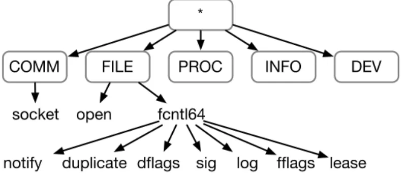
The groups introduced in Tab. 18 form the top level of the taxonomy for the system call types (see Fig. 5). The socket call is a child of group COMM and FILE is the parent of calls like open and fcntl64. Subtypes of system calls can be defined by considering the possible values of their parameters. For example, the fcntl64 call which operates on file descriptors has fd, cmd and arg as its parameters. We have divided the 16 different nominal values of the cmd parameter into seven groups — notify, dflags, duplicate, sig, lock, fflags and lease — that have become the children of the fcntl64 system call in our taxonomy (see Fig. 5). One may further divide fcntl64 calls of subtype fflags by the values F SETFL and F GETFL of the arg parameter. In the same way, we defined parents and children for each of the 54 call types and their parameters.

*

COMM FILE PROC INFO DEV

socket open fcntl64 duplicate dflags

notify sig log fflags lease

Fig. 5. Parts of the taxonomy we defined for the hierarchical variable system call type.

Albeit the taxonomy we present here already yields promising results in our experiments, we consider it to be an open research question how to find a cate- gorization of system calls that fits a given learning task.

The hierarchical variable file path is defined whenever a system call accesses a file system path. Its hierarchy comes naturally along with the given file path hierarchy of the file system. The call sequence variable expresses the temporal order of calls within a process. The directly preceding call is the highest, less recent calls are at deeper levels of the hierarchy. The information which is kept in a sequence are the names of the system calls.

Collected data We have implemented a parser that reads log files and trans-

lates them into hierarchical value tupels according to the three taxonomies

Application Version Function Firefox 3.0.15 Webbrowser

top 3.2.7 Display of running processes Rhythmbox 0.12.0 Audio player

Geyes 2.26.1 Eyes following mouse pointer

NEdit 5.5 Text editor

Vinagre 2.26.1 Remote control XEmacs 21.4.21 Text editor

Kate 3.2.2 Text editor

xterm 241 Terminal emulator

Tomboy 0.14.0 Editor for notes Epiphany 2.26.1 Webbrowser

Table 19. List of applications for which system calls were logged.

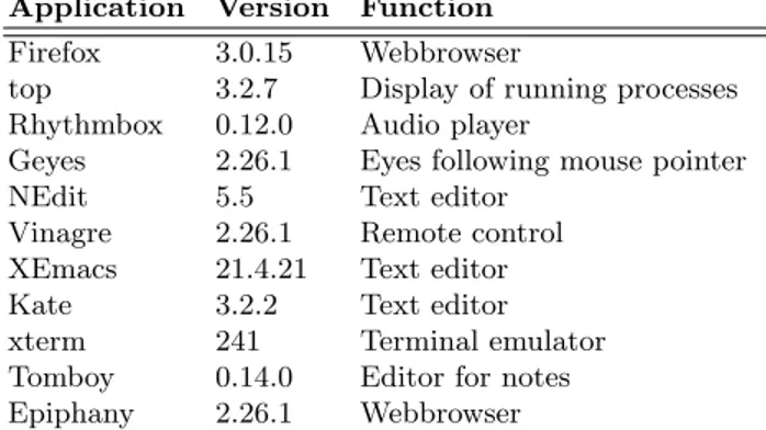
We collected system call data from eleven applications (like Firefox, Epiphany, NEdit, XEmacs) shown in Tab. 19 under Ubuntu Linux (kernel 2.6.26, 32 bit).

For each application, we logged five times five minutes and five times ten minutes of system calls if they belonged to one of the 54 types shown in Tab. 18, resulting in a whole of 110 log files comprising about 23 million of lines (1.8 GB).

3.3 Resulting Aggregation through Hierarchical Heavy Hitters We have implemented the Full Ancestry and Partial Ancestry variants of the HHH algorithm mentioned in Section 3.1. The code was integrated into the RapidMiner data mining tool.

Regarding run-time, all experiments were done on a machine with Intel Core 2 Duo E6300 processor with 2 GHz and 2 GB main memory.

Since we want to aggregate system call data on devices that are severely limited in processing power and available memory, measuring the resource usage of our algorithms was of paramount importance. Table 20 shows the run-time and memory consumption of the Full Ancestry and Partial Ancestry algorithms using only the system call type hierarchy, the system call type and file path hierarchy, or the system call type, file path, and call sequence hierarchy. Minimum, maximum and averages were calculated over a sample of the ten gathered log files for each of the eleven application by taking only the first log file for each application into account.

Memory consumption and run-time increase with the dimensionality of the elements, while at the same time approximation quality decreases. Quality is measured as similarity to the exact solution. Full Ancestry has a higher ap- proximation quality in general. The results correspond to observations made by Cormode and are probably due to the fact that Partial Ancestry outputs bigger HHH sets, which was the case in our experiments, too. Note that approximation

7

The code and all data which was used in the experiments is available at

http://www-ai.cs.uni-dortmund.de/SOFTWARE/HHHPlugin/.

Memory Run-time Similarity

Min Max Avg Min Max Avg Avg Dev

T 19 151 111 16 219 79 0.997 0.006

FA TP 25 9,971 5,988 31 922 472 0.994 0.003

TPS 736 73,403 48,820 78 14,422 6,569 0.987 0.008

T 7 105 70 15 219 74 0.985 0.010

PA TP 7 4,671 2,837 31 5,109 2,328 0.957 0.017

TPS 141 18,058 10,547 78 150,781 74,342 0.921 0.026 Table 20. Memory consumption (number of stored tupels), run-time (milliseconds) and similarity to exact solution of the Full Ancestry (FA) and Partial Ancestry (PA) algorithms (ε = 0.0005, φ = 0.002). Minimum (Min), maximum (Max) and average (Avg) values were calculated over measurements for the first log file of all eleven ap- plications with varying dimensionality of the element tupels (T = system call type hierarchy, P = file path hierarchy, S = call sequence hierarchy).

quality can always be increased by changing parameter ε to a smaller value at the expense of a longer run-time. Figure 6 shows the behaviour of our algorithms on the biggest log file (application Rhythmbox) for three dimensions with vary- ing ε and constant φ. Memory consumption and quality decrease with increasing ε, while the run-time increases. So the most important trade-off involved here is weighting memory consumption against approximation quality — the run-time is only linearly affected by parameter ε. Again, Full Ancestry shows a better approximation quality in general.

Even for three-dimensional elements, memory consumption is quite low re- garding the number of stored tuples. The largest number of tuples (73,403), only equates to a few hundred kilobytes in main memory! The longest run-time of 150,781 ms for Partial Ancestry in three dimensions relates to the size of the biggest log file (application Rhythmbox).

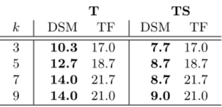
Classification results For the 110 log files of all applications, we determined the HHHs, resulting in sets of frequent tupels of hierarchical values. Interpreting each HHH set as an example of application behaviour, we wanted to answer the question if the profiles could be separated by a classifier. So we estimated the expected classification performance by a leave-one-out validation for kNN.

Therefore, we needed to define a distance measure for the profiles determined by HHH algorithms. The data structures of HHH algorithms contain a small subset of prefixes of stream elements.

The estimated frequencies f

are calculated from such data structure by the output method and compared to φ, thereby generating a HHH set. The similarity measure DSM operates not on the HHH sets, but directly on the internal data structures D

, D

of two HHH algorithms:

sim(D

, D

) = P

p∈P1∩P2

contrib

(p)

|P

∪ P

| .