Estimating Fisheries Reference Points from Catch and Resilience

Estimating Fisheries Reference Points from Catch and Resilience

Rainer Froese, GEOMAR Helmholtz Centre for Ocean Research Kiel, Düsternbrooker Weg 20, 24105 Kiel, Germany, rfroese@geomar.de , +494316004579, Fax +494316001699, corresponding author

Nazli Demirel, Institute of Marine Sciences and Management, Istanbul University, 34134, Istanbul, Turkey, ndemirel@istanbul.edu.tr

Gianpaolo Coro, Istituto di Scienza e Tecnologie dell’Informazione “A. Faedo”, Consiglio Nazionale delle Ricerche (CNR), via Moruzzi 1, 56124 Pisa, Italy. gianpaolo.coro@isti.cnr.it

Kristin M. Kleisner, National Oceanographic and Atmospheric Administration, Northeast Fisheries Science Center, 166 Water St., Woods Hole, MA 02543, kristin.kleisner@noaa.gov

Henning Winker, South African National Biodiversity Institute, Kirstenbosch Research Centre, Claremont 7735, South Africa and Centre for Statistics in Ecology, Environment and Conservation (SEEC),

Department of Statistical Sciences, University of Cape Town, Private Bag X3,Rondebosch 7700, South Africa, henning.winker@gmail.com

Running Title: Reference points from catch & resilience

Alternative title: Monte-Carlo analysis of catch data for data-limited stocks 1

2 3 4 5 6 7 8 9 10 11 12 13 14 15 16 17 18 19 20

Abstract

This study presents a Monte Carlo method (CMSY) for estimating fisheries reference points from catch, resilience, and qualitative stock status information on data-limited stocks. It also presents a Bayesian state-space implementation of the Schaefer production model (BSM), fitted to catch and biomass or catch per unit of effort (CPUE) data. Special emphasis was given to derive informative priors for productivity, unexploited stock size, catchability, and biomass from population dynamics theory. Both models gave good predictions of the maximum intrinsic rate of population increase r, unexploited stock size k and maximum sustainable yield MSY when validated against simulated data with known parameter values. CMSY provided, in addition, reasonable predictions of relative biomass and exploitation rate.

Both models were evaluated against 128 real stocks, where estimates of biomass were available from full stock assessments. BSM estimates of r, k, and MSY were used as benchmarks for the respective CMSY estimates and were not significantly different in 76% of the stocks. A similar test against 28 data-limited stocks, where CPUE instead of biomass was available, showed that BSM and CMSY estimates of r, k, and MSY were not significantly different in 89% of the stocks. Both CMSY and BSM combine the production model with a simple stock-recruitment model, accounting for reduced recruitment at severely depleted stock sizes.

Keywords: Monte Carlo method, Bayesian state-space model, surplus production model, stock- recruitment relationship, data-limited stock assessment, biomass dynamic model

21 22 23 24 25 26 27 28 29 30 31 32 33 34 35 36 37 38 39 40 41 42 43

Contents 1 Introduction

2 Material and methods

2.1 General description of method

2.2 Selection of real stocks and generation of simulated stocks 2.3 CMSY analysis

2.3.1 Determining the boundaries of the r-k space 2.3.2 Setting prior biomass ranges

2.3.3 Finding viable r-k pairs

2.3.4 Finding the most probable values of r, k, MSY and predicted biomass 2.4 Bayesian Schaefer analysis

2.4.1 Transforming r-k bounds into informative priors 2.4.2 Determining a prior for catchability

2.4.3 Implementation of the Bayesian Schaefer model 3 Results

3.1 Results for selecting priors with default rules for r, k, q, and biomass 3.2 Results for simulated stocks with catch and biomass

3.3 Results for fully-assessed stocks

3.4 Results for simulated stocks with catch and CPUE 3.5 Results for data-limited stocks

44 45 46 47 48 49 50 51 52 53 54 55 56 57 58 59 60 61 62 63

4 Discussion

4.1 Diversity of examined stocks 4.2 Priors for r, k, and biomass

4.2.1 How useful was resilience from FishBase for determining prior ranges of r?

4.2.2 Other options for obtaining prior ranges for r

4.2.3 Using maximum catch for obtaining prior ranges for k

4.2.4 Is the use of known stock status as prior for biomass circular logic?

4.2.5 Data requirements of CMSY compared to other methods 4.3 Interpretation of the Schaefer equilibrium curve

4.4 Pragmatic combination of surplus production with recruitment 4.5 Performance of the Bayesian Schaefer model

4.6 Understanding the CMSY triangle 4.7 Performance of CMSY

4.8 Using CMSY for management of data-limited stocks 5 Conclusions

6 Acknowledgements 7 References

64 65 66 67 68 69 70 71 72 73 74 75 76 77 78 79 80 81

1 Introduction

Most commercially exploited fish stocks in the world lack formal fisheries reference points (Froese et al.

2012, Zhou et al. 2012) and thus, the degree of exploitation and the status of the stocks are largely unknown. However, legislation in New Zealand (MFNZ 2008), Australia (DAFF 2007), the U.S. (MSA 2007), and recently also in the European Union (CFP 2013) requires management of all exploited stocks, including those with limited data. Several methods for the assessment of data-limited stocks have been developed (e.g., MacCall 2009; Cope and Punt 2009; Dick and MacCall 2011; Punt et al., 2011; Thorson et al., 2012; Carruthers et al., 2014) and recent reviews of these methods (ICES 2014; Rosenberg et al.

2014) have found the Catch-MSY method of Martell and Froese (2013) to be a promising approach. This study revisits the Catch-MSY method, addresses its shortcomings, namely the biased estimation of unexploited stock size and productivity, and adds estimation of biomass and exploitation rate. It also addresses a general shortcoming of production models, namely the overestimation of productivity at very low stock sizes (Schnute and Richards 2002; ICES 2014). The predictions of the new method (CMSY) are validated against 48 simulated stocks and evaluated against 159 fully or partly assessed real stocks.

2 Material and methods

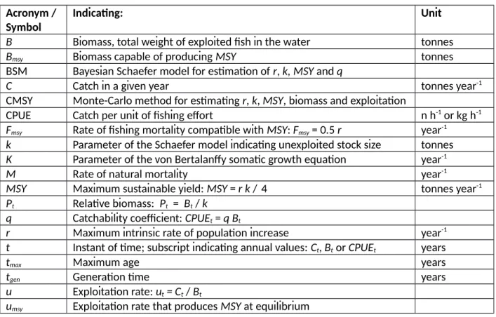
All data files, the R-code of the methods and the figures, a Supplement with detailed presentation of the methods, default rules for priors, and results for 48 simulated and 159 real stocks, and a short text on how to use CMSY are available online for download from http://oceanrep.geomar.de/33076/. For convenience, the acronyms and symbols used in this study are summarized in Table 1.

[Table 1 near here]

2.1 General description of method

A time series of catches can be viewed as a sequence of yields produced by the available biomass with a given productivity. If two of the three variables, yield, biomass, and productivity, are known, then the 82

83 84 85 86 87 88 89 90 91 92 93 94 95

96 97 98 99 100 101

102 103 104

third can be estimated. Typical production models, such as the one by Schaefer (1954), use time series of catch and abundance to estimate productivity. Instead, the CMSY method presented in this study uses catch and productivity to estimate biomass, providing substantial advancement on the Catch-MSY method of Martell and Froese (2013), which focuses on the estimation of maximum sustainable yield (MSY). CMSY estimates biomass, exploitation rate, MSY, and related fisheries reference points from catch data and resilience of the species. Probable ranges for the maximum intrinsic rate of population increase (r) and for unexploited population size or carrying capacity (k) are filtered with a Monte Carlo approach to detect ‘viable’ r-k pairs. A parameter pair is considered ‘viable’ if the corresponding biomass

trajectories calculated with a production model are compatible with the observed catches in the sense that predicted biomass does not become negative, and is compatible with prior estimates of relative biomass ranges for the beginning and the end of the respective time series. Under these conditions, a plot of viable r-k pairs typically results in a triangular-shaped cloud in log-space (Figure 1). The Catch- MSY algorithm (Martell and Froese 2013) was designed to select the most probable r-k pair as the geometric mean of this distribution. CMSY differs from the Catch-MSY method by searching for the most probable r not in the center but rather in the tip-region of the triangle. This is based on the underlying principle that defines r as the maximum rate of increase for the examined population, which should be found among the highest viable r values. In other words, a given time series of catches could be explained by a wide range of large stock sizes and low productivity, or by a narrow range of small stock sizes and high productivity, such as in the tip of the triangle (Figure 1). Since r is defined as maximum net productivity (Schaefer 1954; Ricker 1975), the tip of the triangle is where it should be found.

[Figure 1 near here]

For verification, the predictions of the CMSY method are compared against simulated data where the

“true” values of parameters and biomass data are known. For evaluation against real world fisheries, the predictions of the CMSY method are compared against corresponding parameters and abundance 105

106 107 108 109 110 111 112 113 114 115 116 117 118 119 120 121 122 123 124 125 126 127 128

estimates derived from fully or partly assessed stocks, where biomass or catch-per-unit-effort (CPUE) data are available in addition to catch data. For this purpose, a Bayesian state-space implementation of the Schaefer model (BSM) is developed, where r, k and MSY are predicted from catch and abundance data. The basics biomass dynamics are governed by Equation 1:

B_t+1=B_t+r

(

)

where Bt+1 is the exploited biomass in the subsequent year t+1, Bt is the current biomass, and Ct is the catch in year t.

To account for depensation or reduced recruitment at severely depleted stock sizes, such as predicted by all common stock-recruitment functions (Beverton and Holt 1957; Ricker 1975; Barrowman and Myers 2000), a linear decline of surplus production, which is a function of recruitment, somatic growth and natural mortality (Schnute and Richards 2002), is incorporated if biomass falls below ¼ k (Equation 2).

B_t+1=B_t+4B_t

k r

(

)

The term 4 Bt/k assumes a linear decline of recruitment below half of the biomass that is capable of producing MSY.

The BSM was implemented as a Bayesian state-space estimation model (Meyer and Millar 1999; Millar and Meyer 1999), which allowed accounting for variability in both population dynamics (process error) and measurement and sampling (observation error) (Thorson et al. 2014)

The parameters estimated by CMSY and BSM relate to standard fisheries reference points such that MSY

= r k / 4, the fishing mortality corresponding to MSY is Fmsy = 0.5 r, the biomass corresponding to MSY is Bmsy = 0.5 k (Schafer 1954; Ricker 1975), and the biomass below which recruitment may be compromised is half of Bmsy (Carruthers et al. 2014; Froese et al. 2015; Haddon et al. 2012).

129 130 131 132

133

134 135 136 137 138 139

140

141 142 143 144 145 146 147 148 149

2.2 Selection of real stocks and generation of simulated stocks

Altogether 128 fully assessed stocks with biomass data, 28 data-limited stocks with CPUE data, and three stocks with less than 9 years of abundance data were used for the evaluation of the CMSY method. Catch and biomass data were extracted from stock assessment documents that were available online or were provided by the respective assessment bodies for the Pacific, North and South Atlantic, the

Mediterranean and the Black Sea (see online Supplement for details). In addition to the real stocks, forty-eight simulated stocks with catch and abundance data were created. The goal was to create a range of biomass scenarios, including strongly as well as lightly depleted stocks, with monotone stable or monotone changing (i.e., steadily decreasing or increasing) or with alternating biomass trajectories (see online Supplement for details).

2.3 CMSY analysis

2.3.1 Determining the boundaries of the r-k space

In order to determine prior r ranges for the species under assessment, the proxies for resilience of the species as provided in FishBase (Froese et al. 2000; Froese and Pauly 2015) were translated into the r- ranges shown in Table 2.

[Table 2 near here]

Next, a prior range for k was derived based on three assumptions. First, unexploited stock size k is larger than the largest catch in the time series, because it is highly unlikely that a fishery finds and catches, in a single year, all individuals of a previously unexploited stock (Vasconcellos and Cochrane 2005; Martell and Froese 2013). Thus, maximum catch in the time series was used to inform the lower bound of k.

Second, the maximum sustainable catch expressed as a fraction of the available biomass (Fmsy) depends on the productivity of the stock. This relationship was accounted for by dividing maximum catch by the upper and lower bound of r and using these values as the benchmarks for the lower and upper bounds 150

151 152 153 154 155 156 157 158 159

160 161 162 163 164 165 166 167 168 169 170 171 172

of k. Third, maximum catch will constitute a larger fraction of k in substantially depleted rather than lightly depleted stocks. These considerations are summarized in Equations 3 and 4. Suitable ranges for the catch/productivity ratios were determined empirically with simulated data where the true value of k was known.

k_low=max(C)

r_{hi gh} , k_high=4max ⁡(C)

r_low ⁽³⁾

where klow and khigh are the lower and upper bounds of the prior range of k, max(C) is the maximum catch in the time series, rlow is the lower bound of the range of r values that the CMSY method will explore, and rhigh is the upper bound of that range.

k_low=2max(C)

r_high , k_high=12max ⁡(C)

r_low ⁽⁴⁾

where variables and parameters are as defined in Equation 3.

Equation 3 was applied to stocks with low prior biomass at the end of the time series and Equation 4 was applied to stocks with high biomass. To reduce the influence of extreme catches, catch data were smoothed by a three-year moving average.

2.3.2 Setting prior biomass ranges

In order to provide prior estimates of relative biomass at the beginning and end of the time series, and optionally also in an intermediate year, one of the possible three broad biomass ranges shown in Table 3 was chosen, depending on the assumed depletion level. This was done automatically by default rules described in the online Supplement. Obvious wrong priors resulting from the default rules, such as setting initial biomass to medium when instead the stock was still lightly exploited or already severely depleted at the beginning of the time series, were noted and subsequently adjusted manually. Thus, the results of this study refer to a scenario where managers are assumed to not have made gross errors in 173

174 175 176

177

178 179 180

181

182 183 184 185 186 187 188 189 190 191 192 193

setting broad prior biomass ranges. For example, experts attending the ICES WKLIFE IV and V workshops in Lisbon in October 2014 and 2015 were able to describe stock-status and exploitation histories for some of the North Atlantic stocks, which were then translated into the corresponding relative biomass ranges given in Table 2 (ICES 2014, 2015).

[Table 3 near here]

2.3.3 Finding viable r-k pairs

For the detection of viable r-k pairs, a random r-k pair is selected from within the prior ranges for r and k.

Then, a starting biomass is selected from the prior biomass range for the first year and Equation 1 or 2 is used to calculate the predicted biomass in subsequent years. An r-k pair is discarded if any of the following conditions applies:

1. The predicted biomass is smaller than 0.01 k (the stock crashes);

2. The predicted biomass falls outside the prior biomass range of the intermediate year;

3. The predicted biomass falls outside the prior biomass range of the final year;

If none of these conditions apply, then the r-k pair and the trajectory of predicted biomass are

considered viable and are stored for analysis. For the purpose of this study, this process was applied to 10,000 – 200,000 random r-k pairs, 11-21 start-biomass values, and 3-6 random error patterns for each r-k-start-biomass combination. In order to speed up processing, the search for viable r-k pairs is terminated once more then 1,000 pairs are found. For triangles with a thin tip an additional search is conducted in the tip region.

2.3.4 Finding the most probable values of r, k, MSY and predicted biomass

CMSY seeks the most probable r-k pair near the tip of the triangle of viable pairs (Figure 1). For this purpose, all viable r-values are assigned to 25-100 bins of equal width in log-space. The 75^th percentile of the mid-values of occupied bins is taken as the most probable estimate of r. This procedure gives equal 194

195 196 197 198 199 200 201 202 203 204 205 206 207 208 209 210 211 212 213 214 215 216

weight to all occupied bins and reduces the bias caused by the triangular (instead of ellipsoid) shape of the cloud of viable r-k pairs (compare cloud of probable r-k pairs estimated by BSM in Fig. 1).

Approximate 95% confidence limits of the most probable r are obtained as 51.25^th and 98.75^th percentiles of the mid-values of occupied bins, respectively.

The most probable value of k is determined from a linear regression fitted to log(k) as a function of log(r), for r-k pairs where r is larger than median of mid-values of occupied bins, with log(4 MSY) as intercept and with a fixed slope of -1, based on the rearranged Schaefer model shown in Equation 5.

Note that all r-k pairs on this line have the same intercept and thus give the same value of MSY.

MSY=r k

4 →log(k)=log(4MSY)+(−1)log(r) ₍₅₎ Approximate 95% confidence limits of k are obtained by adding the standard deviation of the residuals of the regression line to the predicted k value at the lower confidence limit of r, and subtracting it from the k-value predicted for the upper confidence limit of r. MSY and its 95% confidence limits are obtained as geometric mean of the MSY values calculated for each of the r-k pairs where r is larger than the median.

Viable biomass trajectories were restricted to those associated with an r-k pair that fell within the confidence limits of the CMSY estimates of r and k. The median of the predicted biomass values for each year was used as the most probable biomass and the 2.5^th and 97.5^th percentiles were used as indicators of the range that contained 95% of the biomass predictions.

2.4 Bayesian Schaefer analysis

2.4.1 Transforming r-k bounds into informative priors

For BSM, the uniform r-ranges shown in Table 2 were translated into prior densities with a central value.

An examination of the density of the viable r-values resulting from CMSY analysis of simulated data was performed using a ²-test against several standard distributions. The results confirmed that r is log- 217

218 219 220 221 222 223 224

225 226 227 228 229 230 231 232 233 234 235

236 237 238 239

normally distributed and suggested that the mean of the r-ranges Table 2 provided a reasonable central value. The height of the density function was inversely related to the width of the r-range, best fit by an inverse range factor (irf) (Equation 6). The standard deviation of r in log-space was then described by a uniform distribution between 0.001 irf and 0.02 irf.

irf= 3

(r_high−r_low) ⁽⁶⁾

where irf is an inverse range factor used in determining the prior density of r for BSM, and rhigh and rlow

indicate the prior r range as defined in Table 2.

The uniform k-ranges used by CMSY (Equations 3 and 4) were translated into a prior density function by assuming that k was log-normally distributed and that the mean of the k-ranges provided a reasonable central value. The standard deviation of the normal distribution in log-space was assumed to be a quarter of the distance between the central value and the lower bound of the k-range (McAllister et al.

2001).

2.4.2 Determining a prior for catchability

Data-limited stocks have, by definition, no estimation of biomass but may have, at least for some years, an estimation of stock abundance as CPUE in units of numbers per hour of fishing or as a biomass index derived from survey catches. Such an abundance index is related to stock biomass by a catchability coefficient q (Equation 7).

CPUE_t=q B_t

(7)

where CPUEt is mean catch per unit effort in year t, Bt is available biomass in year t, and q is the catchability coefficient. The basic dynamics of the corresponding Schaefer production model for abundance as CPUE can therefore be expressed in the form of Equation 8.

240 241 242 243

244

245 246 247 248 249 250 251 252 253 254 255 256 257 258 259 260 261

CPUE_t+1=CPUE_t+r

(

)

where variables and parameters are as defined in Equation 1 and 7. Priors for q were derived from the Schaefer equilibrium equation for catch (Equation 9).

Y=r B(1−B

k) ₍₉₎

where Y is the equilibrium yield for any given biomass B, and other parameters are as defined in Equation 1.

Setting B/k = 0.5, B = CPUE/q and Y = catch gives q = 0.5 r CPUE / Catch for MSY-level catch and biomass.

Setting B/k = 0.25 for half MSY-level biomass gives q = 0.75 r CPUE / Catch. Suitable multipliers for low and high biomass and prior r ranges were derived empirically from simulated data. For stocks with high recent prior biomass, priors for q were derived as shown in Equation 10 and Equation 11.

q_low=0.25r_pgmCPUE_mean

C_mean ⁽¹⁰⁾

where qlow is the lower prior for the catchability coefficient for stocks with high recent biomass, rpgm is the geometric mean of the prior range for r, CPUEmean is the mean of catch-per-unit-effort over the last 5 or 10 years, and Cmean is the mean catch over the same period.

q_{hi gh}=0.5r_highCPUE_mean

C_mean ⁽¹¹⁾

where qhigh is the upper prior for the catchability coefficient for stocks with high recent biomass, rhigh is the upper prior range for r, and all other variables are as defined in Equation 10 .

For stocks with low recent prior biomass, the multipliers were changed from 0.25 to 0.5 for qlow and from 0.5 to 1.0 for qhigh. Mean catch and CPUE were taken over the last 5 years for species with medium and 262

263 264

265

266 267 268 269 270 271

272

273 274 275

276

277 278 279 280

high resilience or over the last 10 years for species with low or very low resilience. For the Bayesian implementation of the Schaefer model, the q-range was translated into a prior density function by assuming that q was log-normally distributed and that the mean of the log q-range provided a

reasonable central value, with a standard deviation assumed to be a quarter of the distance between the central value and qlow (McAllister et al. 2001). The implementation of BSM for CPUE data used the same settings as applied to observed or simulated biomass (see below). If less than 9 years of CPUE data were available, the Schaefer model was not fit. Instead, CPUE was plotted on a second Y-axis in the plot of biomass predicted by CMSY (see example in Figure 6).

2.4.3 Implementation of the Bayesian Schaefer model

The state-space model implementation of the BSM (Miller and Meyer 1999) for catch and biomass and for catch and CPUE are included in the CMSY R-code, which is available as part of the online Supplement.

The JAGS software (Plummer 2003) was used for sampling the probability distributions of the parameters with the Markov chain Monte Carlo method. To facilitate mixing of the Gibbs samples, annual biomass was expressed relative to the unexploited biomass with Pt = Bt / k (Meyers and Miller 1999). Basic parameter settings included three sampling chains with a chain length of 60,000 steps each and with a burn-in phase of 30,000 steps. For the analysis of output, only every 10^th value was used to reduce autocorrelation. All posterior parameter estimates were assumed to be approximately log-normally distributed, with the median used as the central value and 95% confidence intervals approximated by the 2.5^th and 97.5^th percentiles to find values at which test statistics attain less than 0.05 significance (Gelmann et al. 1995; McAllister et al. 2001; Owen 2013).

281 282 283 284 285 286 287 288 289 290 291 292 293 294 295 296 297 298 299 300

3 Results

3.1 Results for selecting priors with default rules for r, k, q, and biomass

To determine the prior ranges for r, resilience categories (Very low, Low, Medium, High) at the species level were used from www.fishbase.org for fishes and were selected manually for the four stocks of invertebrates. These categories, combined with catch data and prior biomass ranges, led to the detection of viable r-k pairs in 140 of 159 stocks (88%). In 19 stocks the resilience category was changed manually to an adjacent lower or upper category in order to find viable r-k pairs. In about half of these cases (9 of 19), the change was to an upper resilience category, i.e., there was no apparent bias in the default rules towards lower or higher categories.

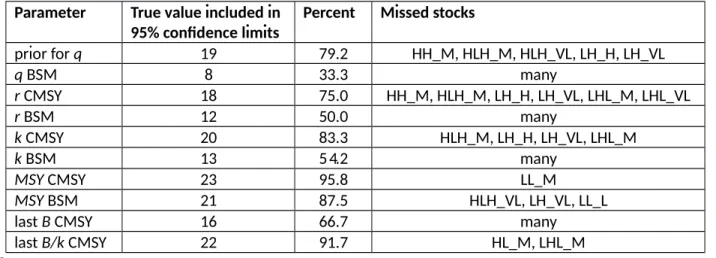
The rules for deriving the prior ranges for k from maximum catch and prior r were sufficient in all cases, no manual adjustments were done. Priors for catchability q were derived from equilibrium reasoning and recent catches (Equations 9-11). The prior ranges included the “true” value of q in 19 of 24 simulated stocks (79%, see Table 8).

To determine prior biomass ranges for the start and end of the time series, and for an optional intermediate year, default rules were used as described in the online Supplement. The resulting prior biomass ranges were compatible with observed biomass or abundance in 92 of 159 stocks (58%). Initial biomass was manually corrected in 14 stocks (9%), intermediate biomass in 11 stocks (9%) and final biomass in 54 stocks (34%). See data on resilience and biomass priors in AllStocks_ID20.xlsx in the online Supplement material.

3.2 Results for simulated stocks with catch and biomass

The CMSY and BSM methods were applied to simulated catch and biomass data where the “true”

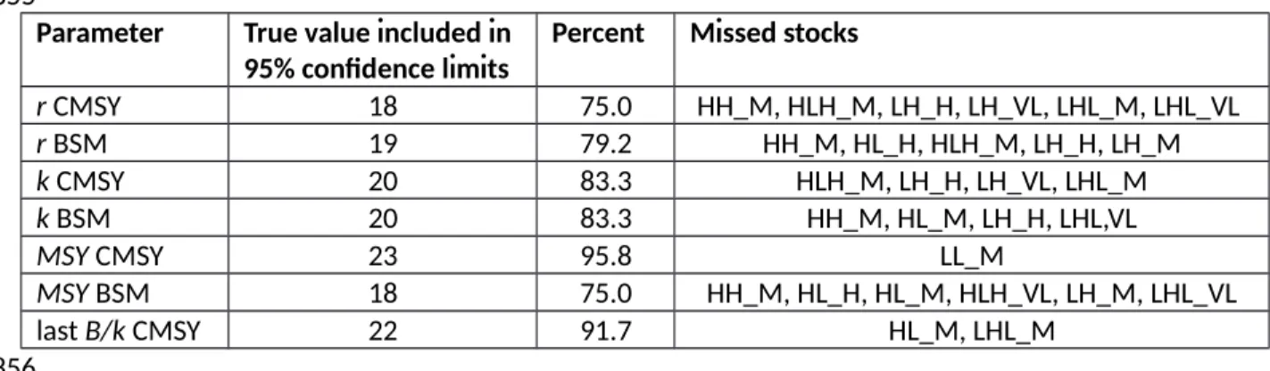
parameter values were known. Tabulated results and detailed analyses for every stock are available in the online Supplement (Tables S3, S4 and Appendix I). In most simulated stocks (75-96%, depending on 301

302 303 304 305 306 307 308 309 310 311 312 313 314 315 316 317 318 319

320 321 322 323

the parameter, see Table 4), the 95% confidence limits of the estimates by CMSY and BSM included the true value used in the simulations and were thus not significantly different from the “true” values (Smith 1995). Results for CMSY and BSM were very similar. Of the six scenarios where CMSY estimates of r did not include the “true” value, four had high final biomass. Similarly, all four scenarios where BSM estimates did not include the “true” value had high final biomass.

A comparison of CMSY and BSM estimates versus “true” values for MSY, r, k, last biomass and last exploitation rate showed that the median ratios and the ranges that contain 90% of the estimates were very similar for both methods (Table 5). The median ratios were close to unity, with maximum deviations of 0.80 and 1.06. The 5^th - 95^th percentile ranges, which contain 90% of the estimates, included the expected ratio of 1.0 in all cases and were bracketed by the ratios 0.69 and 1.62 for BSM and 0.20 and 5.71 for CMSY. The latter strong deviation referred to relative biomass in the simulated stock HL_M. In this case, the “true” value in the final year was 0.002 k, whereas the CMSY estimate was 0.109 k. The deviation is caused by the default prior for low biomass of 0.01 - 0.4 k, which excludes the “true”

biomass.

[Tables 4 and 5 near here]

3.3 Results for fully-assessed stocks

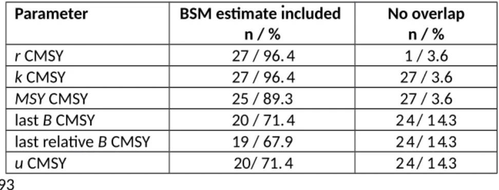
The CMSY and BSM methods were applied to 128 real stocks for which catch and biomass data were available from recent stock assessments. Detailed analyses are available for every stock in Appendix II and summarized in Tables S5 and S6 of the online Supplement. For most stocks (71-79%, depending on the parameter, see Table 6), the 95% confidence limits of the CMSY estimates included the most

probable BSM estimate, indicating good agreement between the methods (Smith 1995). In 5-16% of the stocks the confidence limits of both methods did not overlap, indicating that the predictions were significantly different (Knezevic 2008).

324 325 326 327 328 329 330 331 332 333 334 335 336 337 338

339 340 341 342 343 344 345 346

[Table 6 near here]

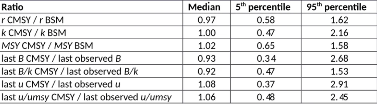
A comparison of CMSY and BSM estimates for MSY, r, k, final biomass and exploitation rate in the final year shows that the median ratios were generally close to 1.0, with maximum deviations of 0.92 and 1.08. The 5^th - 95^th percentile ranges always included unity and were bracketed by the ratios 0.47 and 2.16 for r, k, and MSY, but were wider (0.34 – 2.91) for the last year’s CMSY estimates of biomass and exploitation rate compared to observed data.

[Table 7 near here]

3.4 Results for simulated stocks with catch and CPUE

The CMSY and BSM methods were applied to simulated catch and CPUE data where the true parameter values were known. Tabulated results and detailed analyses for every stock (Appendix III) are available in the online Supplement (Tables S7, S8 and Appendix III). The use of CPUE rather than biomass did not affect the CMSY results, because neither biomass nor CPUE are used by CMSY. The Bayesian

implementation of the Schaefer model for catch and CPUE data required the additional estimation of catchability q in order to transform CPUE into biomass. The 95% confidence limits of q estimated by BSM included the true value in 33% of the cases (Table 8), however with mostly narrow and only three substantial misses (see Table S8 in the online Supplement). For the other parameters (r, k, MSY, last biomass), the 95% confidence limits estimated by CMSY included the true values in 67 - 96% and for BSM in 50 – 88% of the cases (Table 8). The lower success rate of BSM is due to its confidence limits being generally narrower than for CMSY.

[Table 8 near here]

A comparison of CMSY estimates versus true values for MSY, r, k, and last biomass showed median ratios close to 1.0 (0.99 – 1.15) with ranges that contained 90% of the estimates from 0.51 to 5.05. The last number refers to relative biomass in the simulated stock HL_M, where the “true” value in the final year 347

348 349 350 351 352 353

354 355 356 357 358 359 360 361 362 363 364 365 366 367 368 369

was 0.002 k whereas the CMSY estimate was 0.096 k. The deviation is caused by the default prior for low biomass of 0.01 - 0.4 k, which excludes the “true” biomass. The BSM method for data-limited stocks had median ratios of 0.93 to 1.07 and 90% ranges from 0.39 to 6.22, where the latter value stems from the three estimates of q which differed substantially from the “true” value (Table 9).

[Table 9 near here]

3.5 Results for data-limited stocks

Altogether 31 data-limited stocks were analyzed with the CMSY method. Twenty-eight of these stocks had sufficiently long (>= 9 years) time series of abundance available so that BSM could also be applied and CMSY and BSM estimates could be compared. Detailed analyses for every stock as well as summary tables are available in the online Supplement (Appendix IV and Tables S9, S10). In most stocks the 95%

confidence limits of the CMSY estimates for r, k and MSY included the most probable BSM estimate.

Depending on the parameter, the 95% confidence limits of CMSY included the BSM estimate in 68 – 96%

of the stocks (Table 10), suggesting good agreement between the methods (Smith 1995). The confidence limits of both methods did not overlap in 4-14% of the stocks, indicating that the respective estimates were significantly different (Knezevic 2008). A comparison of CMSY and BSM estimates for MSY, r, k, final biomass and exploitation rate in the final year showed that the median ratios and the ranges containing 90% of the estimates were similar for both methods (Table 11). The median ratios were close to 1.0, with maximum deviations of 1.05 and 1.37. The 5^th - 95^th percentile ranges were bracketed by the ratios 0.63 and 1.68 for r, k, and MSY, but were wider (0.51 – 12.8) for the final year estimates of biomass. The strong deviation was caused by two stocks (cod-rock, smn-sp) where biomass was severely depleted to less than 1% of unexploited stock size, while the default biomass prior used by CMSY still assumed 1-40%

of unexploited biomass.

[Tables 10 and 11 near here]

370 371 372 373 374

375 376 377 378 379 380 381 382 383 384 385 386 387 388 389 390 391 392

4 Discussion

4.1 Diversity of examined stocks

We collected 159 time series of catch and abundance from various sources, including stocks from the North and South Pacific, North and South Atlantic, the Caribbean, the Mediterranean and the Black Sea.

Four stocks belonged to two species of crustaceans and the remaining stocks belonged to species of marine fishes, including five elasmobranches. Over two-third of the species were demersal. Other fishes consisted of small pelagic and highly migratory species such as tunas and billfishes. Species were distributed mostly in temperate climate zones, several in subtropical zones, some in polar regions, and only one in the tropics. Deep sea fishes were represented by eleven species. Very low to medium resilience categories were represented by 14 or more stocks each, but only four stocks fell into the high resilience category. Several species were represented by more than one and up to 12 different stocks.

Several time series used in the analysis started as early as 1930 and most reached until 2012. The shortest time series used for CMSY analyses was 11 years. The highest catch was reported for blue whiting (Micromesistius poutassou, Gadidae) with 2.4 million tonnes in the Northeast Atlantic in 2004 and the largest stock size was reported for Eastern Bering Sea pollock (Theragra chalcogramma, Gadidae) with an estimated biomass of 13.1 million tonnes in 1995. This selection of stocks was reasonably complete and representative for the Northeast Pacific and the North Atlantic, but by no means complete or representative for the other areas or for global fisheries. However, the selection of stocks covered a wide range of the diversity of commercial species, suggesting that the methods and default rules for priors used in this study are broadly applicable.

393

394 395 396 397 398 399 400 401 402 403 404 405 406 407 408 409 410 411 412

4.2 Priors for r, k, and biomass

4.2.1 How useful was resilience from FishBase for determining prior ranges of r?

The resilience categories from FishBase (Froese et al., 2000; Froese and Pauly 2015) gave prior ranges of r that led to similar and therefore presumably reasonable CMSY and BSM fits for 88% of the stocks. For the remaining stocks, reasonable fits were only obtained if the next higher or lower resilience category was chosen. The even distribution of these corrections between lower and upper resilience suggests that these species were intermediate to the available resilience categories. Also, for some species, different stocks required different categories. For example, the two examined stocks of surmullet (Mullus surmuletus, Mullidae) gave reasonable fits for CMSY and BSM only when resilience was set Medium for the North Sea stock (mur-347d) and High for the Central Mediterranean stock (mullsur_gsa1516).

Similarly, of the eight examined stocks of haddock (Melanogrammus aeglefinus, Gadidae), seven gave reasonable fits with the FishBase category of Medium resilience, whereas the stock from Georges Bank (Haddock_GB) only gave a reasonable fit when resilience was set to Low. More generally, if the prior r- range is set too high, CMSY is unlikely to find viable r-k pairs; if the prior r-range is set too low, the r-k space is likely to be flooded with viable r-k pairs pressing against the upper bound of r. Thus, while the resilience categories from FishBase provided a good starting point for prior ranges of r, users of the CMSY and BSM methods should carefully consider all available information and then select the most suitable prior range of r for the stock in question, independent of the fixed ranges used for the purpose of this study (Table 2).

4.2.2 Other options for obtaining prior ranges for r

In the context of the Schaefer model, half of the maximum intrinsic rate of population increase r equals the rate of fishing mortality Fmsy that is compatible with MSY (Ricker 1975). Fmsy itself is closely related with the rate of natural mortality M (Zhou et al., 2012; Froese et al., 2014, 2016). Thus, if estimates of 413

414 415 416 417 418 419 420 421 422 423 424 425 426 427 428 429 430 431 432 433 434 435

Fmsy or M are available for other stocks of the respective species, or such estimates are available for similar species in the same area, then these estimates can be used to determine prior ranges for parameter r. Jensen (1996) suggested an evolutionary relationship between natural mortality and the somatic growth parameter K, such that K = 2/3 M. Kenchington (2014) examined 29 estimators of natural mortality and concluded that M = 1.5 K or Pauly’s (1980) empirical estimator based on growth

parameters and temperature or maximum age (tmax) with M = 4.3/tmax can provide useful estimates.

Generation time (tgen) is also a strong predictor for r (Myers et al., 1999; Froese et al., 2000; McAllister et al., 2001). FishBase (Froese and Pauly 2015) has compiled mortality estimates for several hundred species and maximum age and growth studies for several thousand species, including most commercial species. These published parameter estimates can be used to establish prior ranges for r. Equation 12 summarizes the approximate relation between r and other life history parameters that may be more easily available.

r ≈2F_msy≈2M ≈3K ≈3/t_gen≈9/t_{max (12)}

4.2.3 Using maximum catch for obtaining prior ranges for k

There is no simple predictor for the unexploited size of a population because estimates of abundance typically start well after fishing has substantially reduced stock size. However, it is highly unlikely that a fishery catches the whole stock in a single year, and thus it is safe to assume that the maximum catch in a time series will be smaller than the unexploited stock size k. Therefore, maximum catch modulated by productivity was used as a reference point for determining prior ranges of k. It can be argued that catch data are the main input of CMSY and that catch must therefore be treated as unknown when

establishing priors (e.g. Kruschke 2011). However, the prior knowledge used here is not the catch itself but the knowledge that the unknown k must be larger than the maximum catch and that populations with high productivity can sustain larger maximum catches relative to k. For the wide range of species 436

437 438 439 440 441 442 443 444 445 446 447 448

449 450 451 452 453 454 455 456 457 458

and stocks examined in this study, the prior range for k was suitable for CMSY and BSM analyses, and thus seems fit for general use.

4.2.4 Is the use of known stock status as prior for biomass circular logic?

Broad estimates of relative biomass at the beginning and the end of the time series of catches are required inputs for CMSY. For the purpose of this study, these prior biomass ranges were set by default rules as Low, Medium or High (Table 2). The default rules gave satisfactory results in about 2/3 of the stocks. But in 34% of the stocks the prior for final biomass had to be corrected to include, or nearly include, observed abundance. Thus, one third of the analyses presented in this study refer to a case where experts had selected prior biomass ranges that were compatible with the true status of the stock.

While this may sound like circular logic, independent knowledge about stock status often exists and its inclusion in the analysis is then mandatory in a Bayesian context (Gelman et al. 1995; Kruschke 2011) For example, it is well known that the North Sea herring stock (Clupea harengus, Clupeidae, her-47d3) was in reasonably good state in the 1950s, collapsed in the 1970s, and has recovered in recent years.

FishBase gives the resilience of this species as Medium. This very general information combined with the time series of catches suffices to produce CMSY estimates of r, k, MSY, and trajectories of biomass and exploitation that are similar to the respective estimates produced by BSM and by regular stock

assessment (Figure 2).

[Figure 2 near here]

Other examples of well-known stock status histories are Georges Bank cod (Gadus morhua, Gadidae, Cod_GB), which was overfished in the 1980s, collapsed in the 1990s, and has not recovered since, or Arctic cod (Gadus morhua, Gadidae, cod-arct), which was abundant in the early 1950s, was near collapse in 1990, and recovered in recent years.

459 460 461 462 463 464 465 466 467 468 469 470 471 472 473 474 475 476 477 478 479 480

Some preliminary testing of the sensitivity of CMSY to incorrectly set prior biomass ranges was done at the WKLIFE V workshop (ICES 2015). As expected, especially long time series were able to recover from incorrectly set initial or intermediate prior biomass ranges, but not from incorrectly set final biomass ranges, because, by design, final biomass estimates outside the prior range are discarded by the CMSY algorithm.

However, similar constraints also apply to many data-limited and data-moderate assessments based on conventional age-structured models (Ludwig and Walters 1989; Mangel et al. 2013). Firstly, in the absence of complete catch time series that date back to the onset of the fishery, it is typically necessary to enforce reasonable initial or current biomass estimates through informative prior or penalties (e.g.

Punt and Hilborn 1997). Secondly, key parameters such as the natural mortality or the steepness of the assumed spawner-recruitment relationship are often fixed or heavily constrained, due to limited information in the available data (Lee et al. 2011, 2012). This means that other important reference points and thus the outcome of the assessment may be determined a priori (Mangel et al. 2013). By comparison, CMSY admits broad uncertainty in resilience and productivity and may therefore be more robust to model misspecifications (Thorson et al. 2014). In summary, the inclusion of independent knowledge about stock status is neither unique to CMSY nor circular logic but mandatory in a Bayesian- type analysis. CMSY is most sensitive to incorrect setting of final prior biomass, but experts and

stakeholders for a given stock are likely to have reasonably correct knowledge about current stock status.

4.2.5 Data requirements of CMSY compared to other methods

In comparison with other methods proposed for data-limited stock assessment, the requirements of CMSY (catch, qualitative resilience and qualitative stock status) appear modest. For example, the DCAC method (MacCall 2009), which estimates a sustainable catch-level below MSY, requires catch, relative depletion, M and Fmsy/M as inputs. The DB-SRA method (Dick and MacCall 2011), which estimates biomass, MSY, B and exploitation rate, requires catch, relative depletion, M, F /M, B /B and age at 481

482 483 484 485 486 487 488 489 490 491 492 493 494 495 496 497 498 499 500 501 502 503 504

maturity as inputs. The COMSIR method (Vasconcellos and Cochrane 2005), which estimates stock status, production and exploitation rates, requires catch, priors for r and k, relative bioeconomic

equilibrium, and increase of harvest rate over time as inputs. The SSCOM method (Thorson et al., 2013), which predicts stock status and productivity, requires catch, priors for unexploited biomass, initial effort, and parameters of an effort-dynamics model. Reviews of these and other data-limited methods

concluded that the Catch-MSY method (Martell and Froese 2013), of which CMSY is an advanced

implementation, performed best with respect to proportional error in predictions (ICES 2014; Rosenberg et al. 2014).

4.3 Interpretation of the Schaefer equilibrium curve

CMSY and BSM as implemented here do not fit a parabola to yield and biomass data, which requires the assumption of equilibrium conditions, but rather search for the r-k pair that best fits the time series of available data and prior information. Plotting catch and biomass data against an equilibrium surplus production curve often looks unconvincing and may lead to erroneous estimates of MSY and Bmsy if the stock was not in a state of equilibrium (Punt 2003). This is depicted in Figure 3a, which shows CMSY and BSM estimates as well as “true” data points for a simulated stock of low resilience with increasing biomass. All points fall below the equilibrium curve, because catches were consistently less than surplus production throughout the time series, which allowed the stock to increase. Also, the non-overlap of the CMSY estimates with the “true” points and the BSM estimates suggests that the CMSY fit for this stock is not particularly good. By contrast, Figure 3b shows a simulated stock with high resilience and a declining biomass pattern, including phases of increase, decrease, and equilibrium, as indicated by the position of points below, above, and near the equilibrium curve, respectively. The overlap of points suggests good agreement between CMSY and BSM estimates and “true” parameter values.

[Figure 3 near here]

505 506 507 508 509 510 511 512

513 514 515 516 517 518 519 520 521 522 523 524 525 526 527

Production models with equilibrium curves of different shapes have been proposed, but they all share the same anchor points, because zero biomass produces zero yield at the one end, and zero yield results in unexploited biomass at the other end. All models have an intermediate maximum at similar absolute catch and biomass values, as forced by the data (Sparre and Venema 1998; Froese et al., 2011, Thorson et al., 2012). Only the estimation of unexploited biomass and therefore the relative position of the biomass that can produce MSY changes with the choice of the production model, from 0.37 B/k with the Fox (1970) model to 0.5 B/k with the Schaefer (1954) model, and somewhere in between with the Pella- Tomlinson (1969) model, depending on the shape-parameter of that model. The parabolas shown in Figure 3 are from a Schaefer model, representing surplus production derived from the first derivative of the logistic model of population growth. The Schaefer model has fewer assumptions and is more conservative than the other models (it predicts lower equilibrium catch at low biomass, see Figure A1 in the Supporting Information of Froese et al., 2011), and was therefore chosen for the implementation of CMSY in this study. The indentation of the parabolas shown in Figure 3 at stock sizes below 0.25 k results from the inclusion of a stock-recruitment model which assumes reduced recruitment at low stock sizes (see next section).

Equilibrium conditions may arise when the same catch is taken over an extended period of time of at least one generation (Kawasaki 1980; Caddy 1984). Thus, persistent deviations in the annual points from the equilibrium curve are more likely to be found in species with low resilience and long generation time, such as in the simulated species with low resilience in Figure 3a. In contrast, a wide and more evenly distributed scattering of points can be expected in species with high resilience and short generation times, such as simulated in Figure 3b. In summary, while the equilibrium curve is not suitable for

parameter estimation in most situations, it is still useful for understanding the status of the stock and for comparing CMSY and BSM estimates.

528 529 530 531 532 533 534 535 536 537 538 539 540 541 542 543 544 545 546 547 548 549 550

4.4 Pragmatic combination of surplus production with recruitment

Production models have been criticized for not taking into account the widely observed reduction in recruitment at low population sizes. Instead, these models assume an increase in the biomass growth rate dB/dt as biomass approaches zero (Schnute and Richards 2002). In earlier versions of CMSY, this increase in productivity with decreases in biomass led to an overestimation of final biomass in depleted stocks (see respective warnings in ICES 2015, Annex 3). Schnute and Richards (2002) propose to solve the general problem by combining the production model with a recruitment function, but their solution consists of eight interconnected equations with more than eight additional parameters to be estimated.

Here we choose a much simpler approach, assuming a generic stock recruitment function with constant recruitment above 0.25 k and linear decline of recruitment below that threshold, toward zero

recruitment at zero biomass. Such a hockey-stick model of recruitment has been proposed by

Barrowman and Myers (2000), and a threshold around half of Bmsy has been widely adopted as a limit reference point for recruitment overfishing (Beddington and Cooke 1983; Myers et al. 1994; Punt et al.

2013; Carruthers et al. 2014; Froese et al. 2014). A hockey-stick function is combined here with the production model by introducing a multiplier which decreases linearly from 1 to zero at biomass below 0.25 k. This multiplier is assumed to reduce the unknown component that recruitment provides to surplus production (Equation 2). This new “surplus production and recruitment” model is used in CMSY and BSM and gives more realistic estimates of r and k in stocks with extended periods of severely depleted biomass. It also removes the bias in CMSY estimates of final biomass in severely depleted stocks (see YTFlo_MA and her-3a22 in Figure 4, with reasonable predictions of final biomass despite severe depletion). Note that the reduction in recruitment at very low stock sizes (B/k < 0.25) also means that Fmsy = ½ r is not applicable anymore and instead Fmsy B/k = ½ r 4 B/k should be used for management advise.

[Figure 4 near here]

551 552 553 554 555 556 557 558 559 560 561 562 563 564 565 566 567 568 569 570 571 572 573 574

4.5 Performance of the Bayesian Schaefer model

Dynamic production models, such as the implementation of the Schaefer model used in this study, require time series of catch and abundance as inputs and thus do not count as data-limited methods.

However, since CMSY is a simplified Bayesian implementation of a data-limited production model, it seems appropriate to compare CMSY results with the results of a full Bayesian implementation of a surplus production estimation model, rather than with results obtained from various stock assessment methods with different assumptions and often unavailable levels of uncertainty. The Bayesian Schaefer model applied in this study (BSM) is similar to previous implementations (e.g. Meyer and Millar 1999;

MacAllister et al. 2001; Vasconcellos and Cochrane 2005; Thorson et al. 2013), but differs in its emphasis on informative priors for k, based on maximum catch modulated by productivity, for q, based on

equilibrium catch, for r, based on more complex modelling of the distribution of r, and for relative biomass ranges, based on default rules or expert opinion. A state-space model implementation was chosen because explicit modelling of process error and observation error has been shown to result in more realistic posterior distributions of parameters (Ono et al. 2012). The resulting predictions for r, k and MSY were close to the “true” values of the simulated data sets and r/2 was reasonably close to working group estimates of Fmsy in 82% of the stocks with available data (see online Supplement).

In summary, BSM performed well when compared with “true” values of simulated stocks. It could be fitted to all real stocks with at least 9 years of abundance data and produced parameter estimates that were comparable with available working group estimates. Thus, the BSM parameter estimates were chosen as benchmarks for the evaluation of CMSY when applied to real stocks where true parameter values are unknown. Of course, like any production model, BSM will provide unrealistic results if one or more of its key assumptions are violated, caused e.g., by environmental regime shifts, dramatic changes in the productivity or size structure of the stock, or major changes in catchability. Also, in stocks that are 575

576 577 578 579 580 581 582 583 584 585 586 587 588 589 590 591 592 593 594 595 596 597

lightly exploited such as the simulations ending in high biomass, the interplay between catch and biomass contains less information about productivity and estimates of r will be less reliable (see Table 4).

4.6 Understanding the CMSY triangle

The typical triangular shape of viable r-k points in log-space (Figure 1) has a biological basis. The given time series of catches may have been produced either by a large population with low to medium

productivity or by a small population with high productivity. This relation is reflected by the well-defined lower bound of the r-k triangle, which represents for a given r the lowest k that is compatible with the catches and the biomass priors. The slope of this lower border is typically a bit flatter than the slope (-1) of the line of r-k pairs resulting in the same value of MSY (Equation 5). The upper border of the r-k triangle is typically more diffuse, marking the highest k values which, if combined with the corresponding r, will not result in a predicted biomass exceeding the upper prior biomass ranges. Because a large population can support a wide range of modest catch patterns even with low or medium productivity, more viable r-k pairs are found in the upper left low-r-high-k corner of the log r-k space. In contrast, while a small population may be able to support high catches if it has high productivity, such catches will take a large proportion of the population resulting in strong inter-annual fluctuations which are prone to falling outside the theoretical and prior biomass ranges. As a result, few or no viable r-k pairs are found in the lower right high-r-low-k corner of the log r-k space. As a general rule, CMSY will find more viable r- k pairs in stocks where catches take a small fraction of available biomass, and vice versa. In summary, the CMSY-triangle is the result of the Monte Carlo filtering process within a fixed r-k space and with hard prior bounds for biomass. The tip of the triangle typically transverses the expected ellipsoid cloud of viable r-k pairs found by BSM from catch and abundance data. The beauty of CMSY is that it finds this area without knowledge of abundance, albeit with a non-representative distribution. Overcoming the problems created by this triangular rather than ellipsoid distribution is the main achievement of CMSY compared with the Catch-MSY method of Martell and Froese (2013).

598 599

600 601 602 603 604 605 606 607 608 609 610 611 612 613 614 615 616 617 618 619 620 621

4.7 Performance of CMSY

Given the limited amount of input data consisting of catch, qualitative resilience and qualitative stock status, the predictions of CMSY are surprisingly accurate when validated with “true” values of simulated stocks or evaluated against BSM estimates for real stocks. While not every fluctuation of simulated or observed stock abundance is traced, the overall patterns of stock development and exploitation are usually reproduced, as shown in Figure 4 for North Atlantic swordfish (Xiphias gladius, Xiphiidae, Swordfish_NA) and Arctic cod (cod-arct). A preliminary analysis suggests that CMSY will underestimate MSY and k if landings instead of catch data are used and discards are substantial. However, even with landings data, the estimates of r and relative biomass B/k seem to correctly reflect the productivity and the status of the stock (ICES 2014).

4.8 Using CMSY for management of data-limited stocks

The predictions of CMSY can be presented in a format useful for stock assessment and management of data-limited stocks (see Appendix IV in the online Supplement). In the example of Baltic brill

(Scophthalmus rhombus, Scophthalmidae, bll-2232) (Figure 5), catches exceeded MSY in 1995 and from 2008 to 2010, but exploitation was below the MSY-level in recent years. Highly variable CPUE data are available from 2001 onward. Both CMSY and BSM predict biomass between half Bmsy and Bmsy in recent years. This information is summarized in a stock status graph, showing the development of the stock from the high-exploitation-low-biomass danger zone in the lower right quadrant of the graph towards the recovery zone in the upper half of the lower-left quadrant. If the goal is stock-recovery with better future yields, the management advice from this analysis is straightforward: maintain catches at their current low level until both CMSY and BSM predict biomass above Bmsy for 2-3 years in a row. Then increase catches to the lower confidence limit of MSY.

[Figure 5 near here]

622 623 624 625 626 627 628 629 630 631

632 633 634 635 636 637 638 639 640 641 642 643 644

Management advice is less clear for the data-limited stock of blond ray in ICES Division IXa (Raja brachyura, Rajidae, rjh-pore) (Figure 6), where CPUE data are only available from 2008 - 2014, too few for BSM analysis. CMSY predicts that catches were near MSY until 2005 and dropped to below half of MSY thereafter. Biomass recovers toward Bmsy in 2014, however, there is a wide margin of uncertainty around that prediction. CPUE data show little change in biomass from 2008 to 2013 but confirm a drop in exploitation rate. Precautionary management may restrict catches at current levels until additional CPUE data allow for a BSM analysis and confirm a recovery to Bmsy. At that point, the lower 95%

confidence limit of MSY can serve as guidance for allowed catches.

[Figure 6 near here]

If no CPUE data are available, other indicators can be used to confirm the predictions of CMSY analysis before they are used to inform management. For example, mean length in the catch relative to length at first maturity and relative to length at maximum cohort biomass can be used to derive independent evidence of stock status (ICES 2014; Jardim et al. 2014; Froese et al. 2015; ICES 2015).

Given the renewed interest in the MSY concept, it may be worthwhile to repeat the following warning of the Food and Agriculture Organization of the United Nations (FAO), given at an expert consultation on the regulation of fishing effort in Rome, 17–26 January 1983: “Attempts to tune a system for attainment of maximum output (MSY) will lead to oscillation, unpredictability and, because of the inertia of the socio-economic system, eventually to crashes (whether reversible or not). A lower level of output is safer and more predictable” (Caddy 1984). This warning is confirmed by the recent exploitation history of the 128 fully assessed stocks examined in this study: maximum catches had exceeded MSY in 92% of the stocks, resulting in recent biomass below the level that can produce MSY in 58% and potentially reduced recruitment (B/k < 0.25) in 20% of these stocks. Four stocks (3%) were severely depleted (B/k < 0.1). In 645

646 647 648 649 650 651 652 653 654 655 656 657 658 659 660 661 662 663 664 665 666

contrast, all of the 10 stocks where exploitation was kept below MSY had recent biomass levels above the one that can produce MSY, as predicted by the expert consultation in 1983 (Caddy 1984).

5 Conclusions

This study presents a Monte Carlo method (CMSY) for estimating fisheries reference points from catch, resilience, and qualitative stock status in data-limited stocks. It also presents a new Bayesian state-space implementation of the Schaefer production model (BSM), fitted to catch and biomass or CPUE. Both methods consider reduced recruitment and thus reduced productivity at low stock sizes and gave good predictions of r, k and MSY when validated against simulated data. CMSY provides, in addition, reasonable predictions of relative biomass and exploitation rate when compared with “true” simulated data. Both models were also evaluated against 128 real stocks, where estimates of biomass were available from full stock assessments. BSM estimates of r, k, and MSY were used as benchmarks for the respective CMSY estimates. These estimates were not significantly different in 76% of the stocks. A similar test against 28 data-limited stocks, where CPUE instead of biomass was available, shows that BSM and CMSY estimates were not significantly different in 89% of the stocks. Examples for using CMSY in the management of data-limited stocks are given.

6 Acknowledgements

Gianpaolo Coro acknowledges the Pew Charitable Trusts for having supported his participation to the ICES WKLife 4 meeting, 27-31 October 2014, in Lisbon, Portugal. Rainer Froese acknowledges support by the European Union’s Seventh Framework Programme (FP7/2007-2013) under grant agreement

244706/ECOKNOWS project and by the Lenfest Ocean Program at The Pew Charitable Trusts under contract ID 00002841. Nazli Demirel acknowledges support from The Scientific and Technological Research Council of Turkey (TUBITAK). Kristin Kleisner acknowledges support through the National 667

668

669 670 671 672 673 674 675 676 677 678 679 680 681

682 683 684 685 686 687 688

Oceanographic and Atmospheric Administration’s Northeast Fisheries Science Center and The Nature Conservancy with a grant from the Gordon and Betty Moore Foundation. This is FIN contribution number 200.

7 References

Barrowman, N.J. and Myers, R.A. (2000) Still more spawner–recruitment curves: the hockey stick and its generalizations. Canadian Journal of Fisheries and Aquatic Sciences 57, 665–676.

Beverton, R.J.H. and Holt, S.J. (1957) On the dynamics of exploited fish populations. Great Britain Ministry of Agriculture, Fisheries and Food, London.

Caddy, J.F. (1983) An alternative to equilibrium theory for management of fisheries. In FAO (1984) Papers presented at the Expert Consultation on the regulation of fishing effort (fishing mortality). Rome, 17–26 January 1983. A preparatory meeting for the FAO World Conference on fisheries management and development. FAO Fisheries Report No. 289 Suppl. 2, 214 p.

Carruthers, T.R., Punt, A.E., Walters, C.J., MAcCall, A., McAllister, M.K., Dick, E.J. and Cope, J. (2014) Evaluating methods for setting catch limits in data-limited fisheries. Fisheries Research 153, 48-68.

CFP (2013) Regulation (EU) No 1380/2013 of the European Parliament and of the Council of 11

December 2013 on the Common Fisheries Policy, amending Council Regulations (EC) No 1954/2003 and (EC) No 1224/2009 and repealing Council Regulations (EC) No 2371/2002 and (EC) No 639/2004 and Council Decision 2004/585/EC. Official Journal of the European Union L 354, 22-61. Available at:

http://eur-lex.europa.eu/LexUriServ/LexUriServ.do?uri=OJ:L:2013:354:0022:0061:EN:PDF (accessed on 19th December 2014)

689 690 691

692

693 694

695 696

697 698 699 700

701 702

703 704 705 706 707 708

Cope, J. and Punt, A.E. (2009) Length-based reference points for data-limited situations: applications and restrictions. Marine and Coastal Fisheries: Dynamics, Management, and Ecosystem Science 1, 169–186.

DAFF (2007) Commonwealth Fisheries Harvest Strategy: Policy and Guidelines. Australian Government, Department of Agriculture, Fisheries and Forestry, 55 p. Available at:

http://www.agriculture.gov.au/SiteCollectionDocuments/fisheries/domestic/hsp.pdf (accessed on 19th December 2014)

Dick, E.J. and MacCall, A.D. (2011) Depletion-based stock reduction analysis: a catch-based method for determining sustainable yields for data-poor fish stocks. Fisheries Research 110, 331-341.

Fox, W.W. (1970) An exponential yield model for optimizing exploited fish populations. Transaction of American Fisheries Society 99, 80–88.

Froese, R., Branch, T.A., Proelß, A., Quaas, M., Sainsbury, K. and Zimmermann C. (2011) Generic harvest control rules for European fisheries. Fish and Fisheries 12, 340-351.

Froese, R., Coro, G., Kleisner, K. and Demirel, N. (2014) Revisiting safe biological limits in fisheries. Fish and Fisheries, doi: 10.1111/faf.12102/

Froese, R., Demirel, N. and Sampang, A. (2015) An overall indicator for the good environmental status of marine waters based on commercially exploited species. Marine Policy 51, 230-237.

Froese, R., Palomares, M.L.D. and Pauly, D. (2000) Estimation of life-history key facts. p. 167-175 In Froese, R. and Pauly, D. (eds), FishBase 2000: concepts, design and data sources. ICLARM, Philippines, 344 p., available at http://www.fishbase.org/manual/English/key%20facts.htm

709 710

711 712 713 714

715 716

717 718

719 720

721 722

723 724

725 726 727

Froese, R., Pauly, D. eds (2015) FishBase. World Wide Web electronic publication. www.fishbase.org, version (10/2015), accessed at www.fishbase.org in November/December 2015.

Froese, R., Winker, H., Gascuel, D., Sumalia, U.R., Pauly, D. (2016) Minimizing the impact of fishing. Fish and Fisheries, DOI: 10.1111/faf.12146

Froese, R., Zeller, D., Kleisner, K. and Pauly, D. (2012) What catch data can tell us about the status of global fisheries. Marine Biology 159, 1283-1292.

Gelman, A., Carlin, J., Stern, H., and Rubin, D. (1995) Bayesian data analysis. Chapman and Hall, New York.

Haddon, M., Klaer, N., Smith, D.C., Dichmont, C.D. and Smith, A.D.M. (2012) Technical reviews for the Commonwealth Harvest Strategy Policy. FRDC 2012/225. CSIRO. Hobart. 69 p.

Hedderich, J. and Sachs, L. (2015) Angewandte Statistik, Methodensammlung mit R. Springer Verlag, Berlin, 968 p.

ICES (2014) Report of the Workshop on the development of quantitative assessment methodologies based on life-history traits, exploitation characteristics, and other relevant parameters for data-limited stocks (WKLIFE IV), 27-31 October 2014, Lisbon, Portugal. ICES CM 2014/ACOM:54, 243 pp.

ICES (2015) Report of the fifth Workshop on the development of quantitative assessment methodologies based on life-history traits, exploitation characteristics and other relevant parameters for data-limited stocks (WKLIFE V), 5–9 October 2015, Lisbon, Portugal. ICES CM 2015/ACOM:56. 157 pp.

Jardim, E., Azevedo, M. and Brites, N.M. (2014) Harvest control rules for data limited stocks using length- based reference points and survey biomass indices. Fisheries Research, 10.1016/j.fishres.2014.11.013 728

729

730 731

732 733

734 735

736 737

738 739

740 741 742

743 744 745

746 747