Sediment history mirrors Pleistocene aridification in the Gobi Desert (Ejina Basin, NW China)

(1)

Solid Earth, 11, 1375–1398, 2020 https://doi.org/10.5194/se-11-1375-2020

Sediment history mirrors Pleistocene aridification in the Gobi Desert (Ejina Basin, NW China)

Georg Schwamborn^1,2,3, Kai Hartmann¹, Bernd Wünnemann^1,4, Wolfgang Rösler⁵, Annette Wefer-Roehl⁶, Jörg Pross⁷, Marlen Schlöffel⁸, Franziska Kobe⁹, Pavel E. Tarasov⁹, Melissa A. Berke¹⁰, and Bernhard Diekmann²

1Freie Universität Berlin, Applied Physical Geography, 12249 Berlin, Germany

2Alfred Wegener Institute, Helmholtz Centre for Polar and Marine Research, 14473 Potsdam, Germany

3Eurasia Institute of Earth Sciences, Istanbul Technical University, Maslak 34469, Istanbul, Turkey

4East China Normal University, State Key Laboratory of Estuarine and Coastal Research, Shanghai 200241, China

5Department of Geosciences, University of Tübingen, 72074 Tübingen, Germany

6Senckenberg Gesellschaft für Naturforschung, 60325 Frankfurt, Germany

7Institute of Earth Sciences, Heidelberg University, 69120 Heidelberg, Germany

8Institute of Geography, University of Osnabrück, 49074 Osnabrück, Germany

9Institute of Geological Sciences, Freie Universität Berlin, 12249 Berlin, Germany

10University of Notre Dame, Department of Civil and Environmental Engineering and Earth Sciences, Notre Dame, IN 46556, USA

Correspondence:Georg Schwamborn (georg.schwamborn@fu-berlin.de) Received: 22 October 2019 – Discussion started: 4 November 2019

Revised: 28 February 2020 – Accepted: 18 March 2020 – Published: 23 July 2020

Abstract.Central Asia is a large-scale source of dust transport, but it also held a prominent changing hydrological system during the Quaternary. A 223 m long sediment core (GN200) was recovered from the Ejina Basin (synonymously Gaxun Nur Basin) in NW China to reconstruct the main modes of water availability in the area during the Quater- nary. The core was drilled from the Heihe alluvial fan, one of the world’s largest alluvial fans, which covers a part of the Gobi Desert. Grain-size distributions supported by endmember modelling analyses, geochemical–mineralogical compositions (based on XRF and XRD measurements), and bioindi- cator data (ostracods, gastropods, pollen and non-pollen palynomorphs, and n-alkanes with leaf-wax δD) are used to infer the main transport processes and related environmental changes during the Pleistocene. Magnetostratigraphy supported by radionuclide dating provides the age model. Grain- size endmembers indicate that lake, playa (sheetflood), fluvial, and aeolian dynamics are the major factors influenc- ing sedimentation in the Ejina Basin. Core GN200 reached the pre-Quaternary quartz- and plagioclase-rich “Red Clay”

formation and reworked material derived from it in the core bottom. This part is overlain by silt-dominated sediments be-

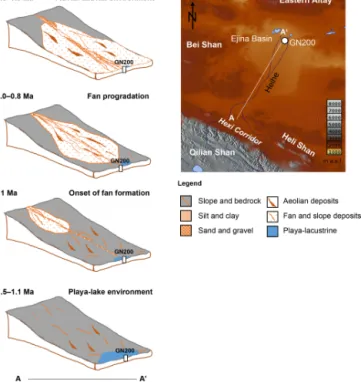
tween 217 and 110 m core depth, which represent a period of lacustrine and playa-lacustrine sedimentation that presum- ably formed within an endorheic basin. The upper core half between 110 and 0 m is composed of mainly silty to sandy sediments derived from the Heihe that have accumulated in a giant sediment fan until modern time. Apart from the transition from a siltier to a sandier environment with frequent switches between sediment types upcore, the clay mineral fraction is indicative of different environments. Mixed-layer clay minerals (chlorite/smectite) are increased in the basal Red Clay and reworked sediments, smectite is indicative of lacustrine-playa deposits, and increased chlorite content is characteristic of the Heihe river deposits. The sediment succession in core GN200 based on the detrital proxy interpretation demonstrates that lake-playa sedimentation in the Ejina Basin has been disrupted likely due to tectonic events in the southern part of the catchment around 1 Ma. At this time Heihe broke through from the Hexi Corridor through the Heli Shan ridge into the northern Ejina Basin. This initiated the alluvial fan progradation into the Ejina Basin. Presently the sediment bulge repels the diminishing lacustrine environment further north. In this sense, the uplift of the hin-

(2)

terland served as a tipping element that triggered landscape transformation in the northern Tibetan foreland (i.e. the Hexi Corridor) and further on in the adjacent northern intraconti- nental Ejina Basin. The onset of alluvial fan formation co- incides with increased sedimentation rates on the Chinese Loess Plateau, suggesting that the Heihe alluvial fan may have served as a prominent upwind sediment source for it.

1 Introduction

The aridification of the Asian interior since ∼2.95–2.5 Ma (Su et al., 2019) is one of the major palaeoenvironmental events during the Cenozoic. The “Red Clay” formation and loess deposits on the Chinese Loess Plateau, which are prod- ucts of the Asian aridification, have been used to broadly constrain the drying history of the Asian interior during the Neogene (Porter, 2007). Studies on these sediment sequences indicate that aeolian deposits started to accumulate on the Chinese Loess Plateau since∼7–8 Ma (Song et al., 2007), suggesting an initiation of Asian aridification during the late Miocene. Cenozoic uplift of the Tibetan Plateau had a pro- found effect upon the desertification in the Asian interior by enhancing it (Guo et al., 2002). The timing of the uplift of the northern Tibetan Plateau has been under debate for decades and is still so today, i.e. the onset of intensive exhumation in the Qilian Shan at the northeastern border of the Tibetan Plateau is thought to occur at ∼18–11 Ma and at approximately 7±2 Ma (Pang et al., 2019). Wang et al. (2017) suggest an emergence of the Qilian Shan during the late Miocene, the area where the Heihe (synonymously Hei River) evolves from its upper reaches on the northern flanks.

River sediments from the Heihe and the more southeast- erly flowing Shiyang River are considered a major source for the Badain Jaran Desert and Tengger Desert (Yang et al., 2012; Li et al., 2014; Wang et al., 2015; Hu and Yang, 2016).

It has been argued that they belong to the dust sources for the Chinese Loess Plateau (Derbyshire et al., 1998; Sun, 2002;

Che and Li, 2013; Pan et al., 2016; Yu et al., 2016). Today, the Heihe flows from the Hexi Corridor through the Heli Shan northwards into the Ejina Basin (synonymously Gaxun Nur Basin), where it forms a giant alluvial fan (Fig. 1). When arriving at the lower reaches of the Heihe, the river carries not only the sediments eroded from the Qilian Shan but also sediments washed from the western Beishan by ephemeral streams and silty sands blown in from Mongolia in the north (Li et al., 2011; Che and Li, 2013). In addition, ephemeral channels originating from the eastern Altay Mountains (synonymously Altai Mountains) indicate that large amounts of sediments are transported from there to the Ejina Basin. Dur- ing the local wet periods of marine isotope stages (MIS) 3 and 5, and the mid-Holocene (Yang et al., 2010, 2011),

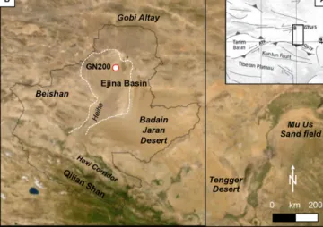
Figure 1. (a)The study site is located in an area dominated by left-lateral transpression due to the ongoing India–Eurasia collision. GTSFS=Gobi Tien Shan fault system, QSTF=Qilian Shan thrust front, ATF=Altyn Tagh fault.(b)White dotted line: Heihe fan covering much of the Ejina Basin. Black line: Heihe catchment.

GN200 marks the coring site. (Service layer credits: Esri, Digital- Globe, GeoEye, Earthstar Geographics, CNES/Airbus DS, USDA, USGS, AeroGRID, IGN, and the GIS User Community. The map was created using ArcGIS^®software. ArcGIS^®is the intellectual property of Esri and is used herein under licence. ©Esri.)

strong fluvial input from the Altay Mountains can be expected (Wünnemann et al., 2007a).

The Ejina Basin has a lateral and vertical set of different sediment archives, i.e. lacustrine, playa-lacustrine, aeolian, and fluvial–alluvial (Wünnemann and Hartmann, 2002; Zhu et al., 2015; Yu et al., 2016). Coring the alluvial fan and underlying deposits at a central position within the basin is thus expected to yield a record that constrains the timing and mirrors the complex interactions between (i) Quaternary climate forcing of the Heihe discharge, (ii) a tectonic triggering of sediment pulses from the uplifting Qilian Shan, and (iii) internal sedimentation dynamics as they are characteristic of downstream alluvial fan progradation.

The purpose of this study is to reconstruct the palaeoenvironmental change driven by climate and tectonic history in the area based on a sediment core from a distal position of the Heihe alluvial fan. The sediment is used for generating sedimentological data (i.e. grain size, XRF, XRD) that are aug- mented by information from selected bioindicators (ostracod and gastropod counts, pollen and non-pollen palynomorphs, n-alkane abundances, andδD values). Based on this multi- proxy dataset, the transition from more humid to more arid conditions in the Ejina Basin during the past 2.5 Ma years is reconstructed.

(3)

G. Schwamborn et al.: Sediment history mirrors Pleistocene aridification 1377 2 Geographical, tectonic, and climatic setting

The Ejina Basin is located in the Gobi Desert and part of the Alashan Plateau. It is an intramontane basin bordered by the Heli Shan in the south, the Beishan to the west, the Badain Jaran Desert to the east, and the eastern Altay Moun- tains to the north (Fig. 1). The Ejina Basin has developed as a pull-apart basin between the northern Tibetan uplands (i.e.

the Qilian Shan) in the south and the Gobi Altay–Tien Shan mountain chain in the north (Becken et al., 2007). There is predominantly a left-lateral transpression acting on the regional upper crust due to the ongoing India–Eurasia collision (Cunningham et al., 1996). Allen et al. (2017, and refer- ences therein) describe that seismicity with earthquake magnitudes M>7 have affected the Qilian Shan and the Hexi Corridor (see Fig. 1) in historic times. Neotectonic activity at the eastern edge of the Ejina Basin was interpreted based on graben geometry detected within crystalline basement using resistivity measurements (Becken et al., 2007; Hölz et al., 2007). Temporal and spatial patterns of fluvial–alluvial and lacustrine deposition are likely influenced by neotectonic movements; e.g. the western basin margin has a sub- sidence rate of ca. 0.8–1.1 m kyr⁻¹(Hartmann et al., 2011), whereas in the northeastern part of the basin the occurrence of seismites illustrates that seismicity has caused sediment rupture in close vicinity to normal fault lines (Rudersdorf et al., 2017). The drilling took place in the centre of the Ejina Basin (42^◦3⁰12.96⁰⁰N, 100^◦54⁰14.4⁰⁰E) at 936 m a.s.l. (above sea level) at a distance to known fault lines.

From south to north, the elevation ranges between 1300 m and 880 m a.s.l. The Heihe main stream entering the Ejina Basin has a length of more than 900 km (X. Li et al., 2018) and originates from the slopes of the Qilian Shan in the south. From its upper reaches, it flows through the foreland of the Hexi Corridor and arrives at the lower reaches with two branches that are likely controlled by fault lines. Here, the Heihe builds up one of the world’s largest alluvial fan systems in the endorheic Ejina Basin (Hartmann et al., 2011).

The Heihe basin covers an area of approximately 28 000 km², while the total catchment of the Heihe system, connected with glaciers in the Qilian Shan (> 4000 m a.s.l.), comprises roughly 130 000 km². Along the distal part of the basin, three terminal lakes, namely Ejina, Sogo Nur, and Juyanze, form a chain of lakes, which presently are all dried up (Wünnemann et al., 2007a). Radiocarbon dating of an- cient shorelines suggests that relative lake-level highstands occurred during MIS 3 (Wünnemann and Hartmann, 2002;

Wünnemann et al., 2007b; Hartmann et al., 2011), although the ¹⁴C-based chronology for the area may underestimate the timing when compared with IRSL OSL (infrared stimulated luminescence optically stimulated luminescence) results (Zhang et al., 2006; Wang et al., 2011; Long and Shen, 2015; Li et al., 2018a, b).

Presently the winter Siberian Anticyclone dominates the climate conditions in the basin (Chen et al., 2008; Mölg et

al., 2013). For the seasonal cycle, Liu et al. (2016) have as- certained that there are strong winds, especially in spring and autumn, with maximum wind speeds of 16.5 m s⁻¹. Westerly winds prevailing during summer in the area thereby inter- act with humid air masses of the summer monsoon further south to release occasional heavy rain fall and thunderstorms (Domrös and Peng, 2012), which may occur at least in the Badain Jaran and Tengger deserts (Wünnemann, 1999).

The study area is characterized by a continental climate that is extremely hot in the summer and cold in the winter;

the maximum daily temperature is 41^◦C (in July) and the minimum daily temperature is−36^◦C (in January). Accord- ing to data from the Ejina weather station between 1959 and 2015, the mean annual temperature, precipitation, relative humidity, and wind speed were 9.0^◦C, 36.6 mm, 33.7 %, and 3.3 m s⁻¹, respectively, and the mean annual potential evap- oration is as high as 3755 mm (Liu et al., 2016). The growing season in the Ejina Basin is from April to September, during which time it is ice free and has seasonal Heihe river runoff.

In contrast, the annual precipitation in the upper reaches in the Qilian Shan reaches 300–500 mm (Wang and Cheng, 1999; Wünnemann et al., 2007a). Today, only the Ejina Oa- sis near Juyanze palaeolake receives ephemeral water input.

Typical geomorphological features in the Ejina Basin are gravel plains, yardangs, playas, sand fields, and sporadically distributed mobile linear and barchan dunes (Zhu et al., 2015;

Yu et al., 2016).

Modern vegetation of the Alashan Plateau and the foothills of the Qilian Shan is dominated by semi-desert and desert plant communities, mainly consisting of shrubs, dwarf shrubs, and low herbs (Herzschuh et al., 2004). Limited in space, steppe vegetation is dominated by various dry- resistant grasses (e.g.Stipa), shrubs, and forb species. Ripar- ian arboreal vegetation typical for the Heihe banks and former river beds is represented byPopulus euphratica,Sophora alopecuroides, and Tamarix ramosissima among the dominant taxa (Herzschuh et al., 2004). Sedge (Carex), grass (Poaceae), and various forb species are typical members of salty meadow and marshy vegetation communities (Hou, 2001).

3 Methods

A rotational drilling system has been used for coring with 3 m long metal tubes 80–120 mm in diameter. Once a core seg- ment was retrieved, it was pressed out immediately, halved, described, and photographically documented. Subtracting core gaps and overlaps, the length of the core is 223.7 m with a recovery rate of 96 %. On average sampling of 2 to 5 cm thick slices was done three times per metre or in accordance with sediment change for studying various sediment properties as described below.

(4)

3.1 Non-destructive analyses

After core splitting, several non-destructive analyses were carried out including visual description, optical line scanning, magnetic susceptibility analyses, and XRF element scanning. Magnetic susceptibility measurements at 1 cm resolution were carried out on one core half using a Barting- ton MS2E sensor, while the other half was scanned with an Avaatech core scanner to semi-quantitatively determine elemental compositions at 1 cm resolution. We applied a rhodium tube at 150 and 175 µA with detector count times of 10 and 15 s for elemental analysis at 10 kV (no filter) and 30 kV (Pd-thick filter). Element intensities were ob- tained by post-processing of the XRF spectra using the Can- berra WinAxil software with standard software settings and spectrum-fitting models. The element intensities depend on the element concentration but also on matrix effects, physical properties, the sample geometry, and hardware settings of the scanner (Tjallingii et al., 2007). We accepted modelled chi-square values (χ²) < 2 as a parameter of measured peak intensity curve fitting for the relevant elements.

3.2 Grain-size distribution and endmember modelling analysis

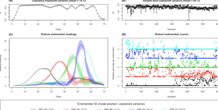
Sediment grain-size distributions were determined using a laser diffraction grain size analyser (Malvern Master- sizer 3000). Prior to laser sizing, the samples were removed from organic carbon using H2O2 oxidation on a platform shaker until reaction ceased. The endmember modelling algorithm (EMMA) after Dietze et al. (2012) and modified by Dietze and Dietze (2019) was applied to the grain size data in order to extract meaningful endmember (EM) grain size distributions and to estimate their proportional contribution to the sediments. Results were translated into a core log that illustrates the succession and thickness of EM types. EM modelling analyses are used to address the main sediment types with their associated transport mechanisms.

3.3 Bulk mineralogy

The mineralogical composition of freeze-dried and milled samples was analysed by standard X-ray diffractometry (XRD) using an Empyrean PANalytical goniometer by applying CuKα radiation (40 kV, 40 mA) as outlined in Petschick et al. (1996). Samples were scanned from 5 to 65^◦ 2θ in steps of 0.02^◦ 2θ, with a counting time of 4 s per step. The intensity of diffracted radiation was calculated as counts of peak areas using XRD processing software (MacDiff, Petschick, 1999). Mineral inspection focused on quartz, plagioclase and K-feldspar, hornblende, mica, calcite, and dolomite. Accuracy of this semi-quantitative XRD method is estimated to be between 5 %–10 % (Gingele et al., 2001).

3.4 Clay mineralogy

The clay fraction (< 2 µm) was separated using settling times according to the Atterberg procedure. Clay particles were oriented using negative pressure below membrane filters and they were mounted as an oriented aggregate mount on alu- minium stubs with the aid of double-sided adhesive tape. The analyses were run from 2.49 to 32.49^◦2θ on a PANalytical diffractometer. Two X-ray diffractograms were performed:

one from the air-dried sample and one from the sample after ethylene glycol vapour saturation was completed for 12 h.

Estimation of clay mineral abundances focused on smectite, mixed-layer smectite/chlorite (10.6 Å), chlorite, and kaolinite (calculated to a sum of 100 %) and is based on peak intensities. Clay analyses were made only from silt-dominated samples.

3.5 Fossil counts

Counts of fossils, i.e. ostracods and gastropods, have been conducted from 62 samples each comprising 40–85 g of dry weight. The size fractions of > 250, 250–125, and 125–63 µm were examined after wet sieving using deionized water. En- countered shells were determined to at least the genus level.

Shell fragments were also registered, but results have been excluded from further discussion due to the assumption that the material points to reworking. To yield meaningful numbers, count results have been normalized to 100 g of dry weight.

3.6 Pollen analysis and biome reconstruction

For pollen analysis, a total of 62 samples (each representing a 2 cm thick layer) was taken from the layers of clayey silt within the 217.2–113 m depth interval with a higher potential for sufficiently good pollen preservation. The samples containing 3 to 5 g of sediment were then treated in the pollen laboratory at the Institute of Geological Sci- ences (FU Berlin) using the dense media separation method as described in Leipe et al. (2019). The laboratory proto- col includes successive treatment of sediment sample with 10 % HCl, 10 % KOH, dense media separation using sodium polytungstate (SPT with a density of 2.1 g cm⁻³), and ace- tolysis. In order to estimate pollen concentration (grains per gram), one tablet with a known quantity of exotic Ly- copodium clavatum marker spores (Batchnr. 483216) was added to each sample prior to the chemical treatment following Stockmarr (1971). At least 200 terrestrial pollen grains were counted in the samples with a concentration of more than 500 pollen grains per gram and a moderate to good pollen preservation. The percentages of terrestrial pollen taxa refer to the total pollen sum taken as 100 %. The percentages of fern spores, aquatic plants, and algae refer to the sum of all pollen and spores. Tilia version 1.7.16 software (Grimm,

(5)

G. Schwamborn et al.: Sediment history mirrors Pleistocene aridification 1379 2011) was used for calculating individual taxa percentages

and drawing the diagram.

Interpretation of pollen records from desert regions is chal- lenging due to several limiting factors, including partially poor pollen preservation, long-distance transport of pollen (e.g. pollen from coniferous and birch trees from mountain forests), and redeposition of pollen from eroded older sediments (Gunin et al., 1999). Modern surface pollen spectra greatly facilitate the interpretation of fossil records from the arid regions (Tarasov et al., 1998). In this study, we used a published set of 55 recent pollen spectra from the Alashan Plateau and Tsilian Shan (Herzschuh et al., 2004). This rep- resentative dataset from the study region helped to establish relationships between pollen spectra composition and modern vegetation, and it was successfully used for interpretation of the Holocene pollen record from the 825 cm long sediment core (41.89^◦N, 101.85^◦E; 892 m a.s.l.) from Juyanze palaeolake (Herzschuh et al., 2004). Pollen-based biome reconstruction is a quantitative approach, which was first de- signed and tested using a limited number of key pollen taxa digitized from the 0 and 6 ka pollen spectra from Europe (Prentice et al., 1996). The method has been further adapted for reconstructing the main vegetation types (biomes) present in northern Eurasia (Tarasov et al., 1998) and in the desert region around the GN200 coring site (Herzschuh et al., 2004).

The latter study presents details of the method and the assign- ment of the terrestrial pollen taxa found in the surface and the Holocene sediment samples from Juyanze core to the respec- tive biomes. In the current study, we apply the same approach and a biome-taxa matrix to the fossil pollen data from the GN200 core as described in Herzschuh et al. (2004).

3.7 Lipid biomarker analysis

Twenty-six samples were used for lipid biomarker analysis. The study focused on determining the concentration and downcore distribution ofn-alkanes in the samples. TheδD values of two n-alkanes (nC₂₉ and nC₃₁) were also measured. Sediment was freeze-dried and homogenized, and 18–

42 g was extracted using a Dionex accelerated solvent extrac- tor 350 with 9:1 dichloromethane–methanol (DCM–MeOH, v:v). The neutral/polar fatty acids and phospholipid fatty acid fractions were isolated from the total lipid extract using an aminopropyl column with 2:1 DCM–2-propanol, 4 % glacial acetic acid in ethyl ether, and MeOH, respectively.

The neutral/polar fraction containing then-alkanes was further separated using an alumina column and 9:1 Hexane–

DCM. A final clean-up column to further separate the satu- rated n-alkanes was run using hexane and silver nitrate on a silica gel column. A Thermo Trace Ultra ISQ gas chro- matograph (GC) mass spectrometer (MS) with flame ion- ization detection (FID) was used to identify and quantify the n-alkanes. Samples were injected in splitless mode at 300^◦C onto a 30 m fused silica column (Agilent J&W DB- 5, 0.25 mm i.d., 0.25 µm film thickness) with hydrogen as

the carrier gas. Following a minute hold at 80^◦C, the GC oven temperature ramped to 320^◦C at a rate of 13^◦C min⁻¹ and with a final hold of 20 min. Then-alkanes were identified by retention times as compared to a standardn-alkanes mix and also by MS fragmentation patterns. An internal standard, 5α-androstane, was used for compound quantification.

The δD values were determined using a Trace 1310 GC coupled to a Finnigan Delta V Plus isotope ratio mass spectrometer (IRMS). Injection conditions and the GC column were identical to measurement on the GC-FID and the oven programme was as follows: 60^◦C isothermal for 1 min, ramp to 320^◦C at 6^◦C min⁻¹, and a 12 min hold at 320^◦C. The H⁺₃ factor was determined daily and averaged 4.8±0.3 ppm mV⁻¹during the analysis. Minimum peak size used was 2500 mV (amplitude 2). Data were normalized to the Vienna Standard Mean Ocean Water (VSMOW) scale using an A6n-alkane standard mix (Arndt Schimmelmann, Indiana University), injected at the beginning, middle, and end of every run for calibration purposes. Squalane with a known isotopic value was co-injected with samples and A6 standard mix to monitor instrument accuracy and precision, and an in-housen-alkane suite was also used to assess instrument conditions. Squalane deviation from the accepted value was < 5 ‰ for all samples and standards analysed. Due to low abundances of other chain lengths, only long-chainn-alkanes (nC₂₉andnC₃₁) were measured forδD values. Alkane data are expressed as concentration (µg g⁻¹dry weight) and using the following equations.

The average chain length (ACL) quantifies the mean ho- mologue length of a suite ofn-alkyl compounds.n-Alkanes (nC19 to nC33) were calculated using Eq. (1). Ci refers to the peak area andirepresents the number of carbons of each individual chain length.

ACL=

P(i ×Ci)

PC_i (1)

Paq quantifies the relative input of non-emergent macrophytes to emergent macrophytes and terrestrial plants (Ficken et al., 2000). The proxy is calculated by the ratio of the sum of abundances of mid-chainn-alkanes to the sum of mid- and long-chain n-alkane abundances as shown in Eq. (2):

P_aq= C₂₃+C₂₅ C23+C25+C29+C31

. (2)

3.8 Statistical treatment

The mineralogical and geochemical data are of compositional nature, which means that they are vectors of non- negative values subjected to a constant-sum constraint (usually 100 %). This implies that relevant information is con- tained in the relative magnitudes, and mineralogical and geochemical data analyses can focus on the ratios between components (Aitchison, 1990). In addition, log transformation

(6)

will reduce the very high values and spread out the small data values, and it is thus well suited for right-skewed distributions (van den Boogaart and Tolosana-Delgado, 2013).

Compared to the raw data, the log-ratio scatter plots exhibit better sediment discrimination.

Log ratios can also minimize the problematic issue that element compositional data from XRF measurements have a poorly constrained geometry (e.g. variable water content, grain size distribution, or density) and non-linear matrix effects (Tjallingii et al., 2007; Weltje and Tjallingii, 2008). In addition, they provide a convenient way to compare different XRF records even when measured on different instruments in terms of relative chemical variations. Log ratios of element intensities are consistent with the statistical theory of compositional data analysis, which allows for robust statistical analyses in terms of sediment composition (Weltje et al., 2015).

Prior to PCA (principal component analysis) andk-means cluster analyses, a centred-log ratio (clr) transformation was applied to the dataset following Aitchison (1990). This means element ratios were calculated from raw cps (counts per second) values and smoothed with a 5 pt (point) running mean. Thus, cps values were clr transformed (Weltje and Tjallingii, 2008), whereby elements measured with 10 kV (Al, K, Ca, Ti, Mn, Fe) were calculated separately from 30 kV elements (Rb, Sr, S, Zr, Cr, Zn, Br).

3.9 Chronostratigraphy

The chronology of core GN200 is derived from magnetostratigraphy. Consolidated sediment samples were cut out manually as specimens and placed in plastic boxes of 1.8 cm×1.8 cm×1.6 cm. A total of 567 samples were used.

Measurements of the natural remanent magnetization (NRM) and stepwise alternating field (AF) demagnetization were performed at the palaeomagnetic laboratory of Tübingen University using a 2G enterprises DC-4 K 755 squid magnetometer system with an in-line 3-axial AF demagnetizer.

For data visualization and interpretation, the software pack- age Remasoft (Chadima and Hrouda, 2006) was used, applying PCA (Kirschvink, 1980) for determination of palaeomagnetic directions. Because no control of drilling azimuths was available, the analysis and interpretation of palaeomagnetic directions is based solely on inclinations. All specimens were subjected to stepwise AF demagnetization (steps: NRM, 4, 6, 8, 10, 15, 20, 25, 30, 40, 50, 60, 80, and 100 mT). Demag- netization runs usually provided interpretable results before reaching the noise level of the magnetometer. The resulting polarity sequence is based on 281 ChRM directions, determined by PCA with a minimum of four consecutive demagnetization steps and mean angular deviation (MAD) < 10^◦ (Fig. 7). A minimum of two subsequent ChRM directions, with inclinations of less than or greater than ±20^◦, was re- quired for defining a polarity interval. Where necessary, also PCA components with MAD > 10^◦or with demagnetization

paths (for the final component) were used to support the interpretation. Overprints of recent Earth magnetic field (EMF;

parallel to normal palaeofield direction), which cannot be separated from the palaeoremanence, lead to better grouping of apparently normal palaeodirections and a more scattered distribution of reverse palaeodirections.

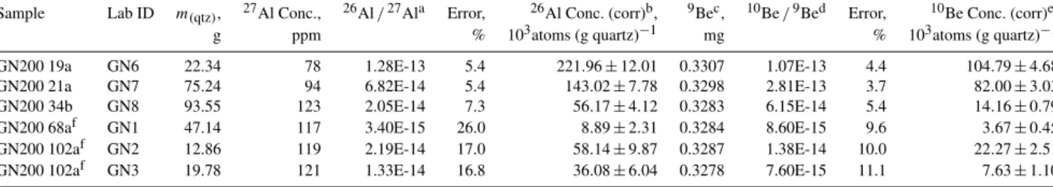
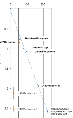
We augment the relative ages of the palaeomagnetic datasets with absolute ages using simple burial dating based on in-situ-produced cosmogenic nuclides (e.g. Balco and Rovey II, 2008; Granger, 2014). Five samples from different depths were sieved, and different grain sizes were cleaned and prepared according to protocols outlined in Schaller et al. (2016). Chemical preparation of the samples was conducted at the University of Tübingen, Germany.¹⁰Be/⁹Be and²⁶Al/²⁷Al ratios were measured at the AMS facility at Cologne, Germany. The age calculation for simple burial dating is based on a MATLAB script by Schaller et al. (2016).

The decay constants used for¹⁰Be and ²⁶Al are (4.997± 0.043)×10⁻⁷ (Chmeleff et al., 2010; Korschinek et al., 2010) and (9.830±0.250)×10⁻⁷, respectively (see Norris et al., 1983). We used sea-level-high-latitude (SLHL) production rates of 3.92, 0.012, and 0.039 atoms (g quartz)⁻¹yr⁻¹ for nucleonic, slow-muonic, and fast-muonic¹⁰Be production, respectively (Borchers et al., 2016; Braucher et al., 2011). The SLHL production rates for ²⁶Al are 28.54, 0.84, and 0.081 atoms (gquartz)⁻¹yr⁻¹for nucleonic, slow- muonic, and fast-muonic production, respectively (Borchers et al., 2016; Braucher et al., 2011). These production rates result in a SLHL²⁶Al/¹⁰Be ratio of∼7.4. We then scaled the SLHL production rates to the sample locations of this study based on the CRONUScalc online calculator of Marrero et al. (2016) using the scaling procedure “SA” from Lifton et al. (2014). Depth scaling of the production rates is based on nucleonic, stopped-muonic, and fast-muonic adsorption lengths, which are 157, 1500, and 4320 g cm⁻², respectively (Braucher et al., 2011). The density of 2.4±0.2 g cm⁻³ is assumed to be constant over the depth of the core.

Depth-to-age transformation was carried out by linear in- terpolation between the ground surface (present) and the core bottom using the palaeomagnetic data; radionuclide results were used for backing up the interpretation.

4 Results

4.1 Sediment stratigraphy

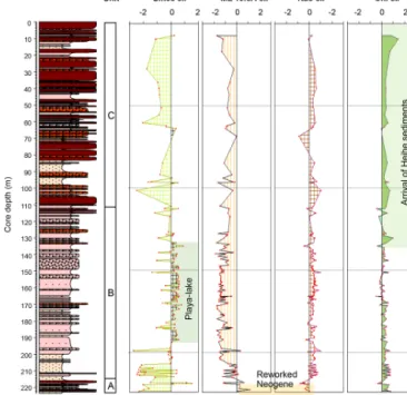
The studied core GN200 was drilled in 2012 to a depth of 223.7 m; three main sedimentary units are identified in it (Fig. 2). Unit A at the core bottom partially belongs to the regionally widespread Red Clay formation, a set of alternating reddish aeolian sediments and carbonate-rich dark- reddish palaeosols of Neogene (Porter, 2007) or Late Cre- taceous (Wang et al., 2015) age. The overlying units B and C represent the Quaternary basin fill and reach a thick-

(7)

G. Schwamborn et al.: Sediment history mirrors Pleistocene aridification 1381

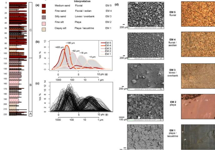
Figure 2. (a)GN200 graphic log with sediment units and litho codes deduced from grain size dominating endmembers (EM) (based on Dietze and Dietze, 2019). Interpretation of depositional environment is added.(b)Illustrated endmember calculation results and(c)sample population (see also Appendix).(d)SEM images and core scan examples for the main sediment types as defined by endmember interpretation.

ness of 222.6 m. From bottom to top, the main macroscopic features are as follows: unit A (223.7–217.0 m) is dominated by coarse-grained layers (fine- to medium-grained sand) interbedded with fine-grained sediments (clayey silt).

Colours change on a sub-metre scale from red and orange in the sandier parts to grey in the silt-rich layers.

Sediment change can be both sharp and transitional. Oc- casionally, centimetre-thick white layers indicate carbonate enrichment in the sandy layers. Unit A includes deposits that are interpreted to belong to the Red Clay formation, i.e. at the core bottom between 223.7 and 222.6 m red sandy clay with angular clasts occurs, which is interpreted a fanglomerate. This subunit has a sharp boundary with the grey (anoxic) medium sand layers overlying them at 222.66 m (see also: http://hs.pangaea.de/Images/Cores/

Lz/Gaxun_Nur/GN200_images_31-223m.pdf, last access:

10 April 2020).

Unit B (217.0–110.0 m) has a succession of banked clayey silt with an increasing frequency of intercalated coarser grained layers dominated by very fine sand to fine sand towards the top of the unit. Silt portions can stretch over several metres upcore and turn from grey (217.0–200.0 m) to brown-

olive colours (200.0–177.0 m). Remarkably, sequences of clayey silt between 210.0 and 200.0 m show successions of millimetre-thick laminations of white and grey-to-orange laminae. Brown to orange colours appear in the middle to upper part of the unit (177.0–110.0 m). Some layers containing coarse sand to very fine gravel form a top subunit (between 120.0–110.0 m). Counts of macrofossils are overall low if samples are not barren at all. Ostracod remains can be found occasionally in layers scattering above 196 m core depth and up to the top of the unit. They are admixed to great- est extent (to double-digit numbers) in coarse silty sediments;

especially at core depths 181.5, 138.0–137.0, 128.0–127.0, 121.0, and at 114.8 m. Gastropod shells are found even more rarely. They are encountered in fine silt at 177.6 and 138.7 m core depth and in coarse silt layers at 120.6 and 113.7 m (fine silt). Remarkably, no fossils occur in the laminated fine silt layers between 210.0 and 200.0 m and between 173.0 and 172.0 m.

Unit C (110.0–0.0 m) is a succession of fine and medium sand layers interbedded with silt banks that decrease in frequency towards the top. The gradational increase in fine silt content in these silt banks is paralleled by a loss of the

(8)

clay fraction. Depending on dominating grain sizes, colours change from yellow, grey, and orange in the sandier layers to light red in the silt banks. At core depths between 28.5 and 27.5 m and between 10.0 and 7.0 m black soft mud occurs, which likely represents lake sedimentation. At 103.2, 99.3, 68.6, and 43.2 m core depths, noteworthy accumula- tions of ostracod shells were found. Dominating grain size fractions in layers containing ostracods range from coarse silt to fine and medium sand. Gastropod shells were found only in few layers at 103.2, 102.9, and 99.9 m depth. The dominating grain-size fractions in these sediments range from coarse silt to fine and medium sand.

A graphic log of the sediment column derived from visual logging and EMMA-derived endmember calculations is presented in Fig. 2. For completion, the sample population and EM modelling results are added. Most of the GN200 samples have a polymodal grain size distribution. The EMMA algorithm produces a five-EM model that envelops all main modes. This explains more than 99.6 % of the total variance (see Appendix). EM 5 is associated with medium to fine sand and a primary mode at∼400 µm and a subordinate mode at 37 µm (8.6 %); EM 4 represents fine sand with the main mode at 180 µm (34 %); EM 3 is composed of silty sand with the main mode at 92 µm (11 %); EM 2 is composed of medium silt with a primary mode at 18 µm and a subordinate mode at 360 µm (27 %). Remarkably, EM 2 is similar to EM 5 but with reverse order of mode precedence. EM 1 is composed of clayey silt with a main mode at 4 µm and a subordinate fine sand fraction admixed (19 %). Surficial processes and landforms producing sediments as found in GN200 are typi- cally fluvial, fluvial-aeolian, levee, and overbank deposition;

sheetflood and surface wash (playa); and lacustrine processes (e.g. Zhu et al., 2015). Apart from unit A, the frequency of coarse-grained (sand-dominated) layers generally increases from the bottom of unit B to the top of unit A. The appear- ance of the first prominent sand layer that is several metres thick in size is used to set the boundary between the two units B and A.

4.2 Dating from palaeomagnetism and radionuclide concentrations

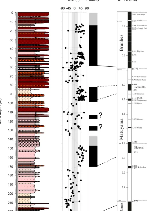
NRM intensities ranged from 0.01–4.2 mA m⁻¹ with a median of 1.6 mA m⁻¹. Most samples exhibited one- component-like or two-component-like demagnetization behaviour. AF demagnetization characteristics and thermomag- netic runs proved magnetite as the main magnetic carrier of the characteristic remanent magnetization (ChRM). The polarity sequence from core GN200 starts at the top with normal polarity and has several longer intervals of reverse polarity further downcore between ca. 60–80, 100–135, and 170–

225 m (Fig. 3). Given that during the Brunhes chron only few very short events of reverse polarity have occurred (Singer, 2014; Cohen and Gibbard, 2019), which cannot explain any longer intervals of reverse polarity, the polarity boundary at

ca. 60 m can be correlated to the Brunhes/Matuyama (B/M) boundary (0.773 Ma). Locating the exact position of the B/M boundary in the record, however, may be a matter of discussion. The EMF behaviour at the B/M boundary is ob- viously rather complex (Singer, 2014), and the limitations of the sampling (no azimuths) and demagnetization proce- dures (no thermal demagnetization possible) do not allow us to disentangle the effects of palaeofield behaviour, lock- in-mechanism, or to separate different palaeofield and recent field components completely. In most of the downcore normal polarity intervals, AF demagnetization of specimens looks like a one-component behaviour, whereas in reverse intervals and near reversals it frequently appears more complex and may exhibit two components of magnetization, which cannot be separated sufficiently. From about 55 to 60 m, shallow normal and reverse components with inclinations < 20^◦ can be observed in many samples. Slightly changing the cri- teria for defining polarity intervals could shift the polarity boundary (B/M boundary) close to 55 m. Based on the polarity pattern and assuming sediment accumulation rates of similar magnitude, the well-defined intervals of normal polarity at about 85–95 and 150–170 m may be tentatively correlated to the Jaramillo (0.988–1.072 Ma) and Olduvai (1.788–

1.945 Ma) sub-chrons. However, it is unclear whether two very short intervals of normal polarity at around 115 and 125 m represent palaeofield behaviour or are artefacts caused by recent field overprints. The lowermost part of the drill core between 172.0 and 222.6 m shows reverse polarity, which is separated by a hiatus from the rest of the polarity sequence.

Burial dating based on in-situ-produced cosmogenic nuclides provides three out of six measurements of¹⁰Be and

26Al concentrations, which have produced reliable results;

namely GN200 19a, GN200 21a, GN200 34b (Tables 1 and 2). In contrast, the remaining three samples produced signals close to blank and are discarded from interpretation (GN200 68a, GN200 102a, GN200 102a, Tables 1 and 2).

The samples from core depths 19.1 m, 20.3 m, and 53.1 m had quartz portions high enough for robust measurements (Tables 1 and 2). The upper two samples have yielded ages > 2 Ma, the one at 53.1 m core depth has an age of 0.84±0.12 Ma (Fig. 4). Given the error bar of the 53.1 m sample (0.84±0.12 Ma), the radionuclide age overlaps with the Brunhes/Matuyama boundary (0.773 Ma) on the geomagnetic timescale and which itself has an error bar of±1 % at this chron boundary (Singer, 2014). If this geochronological interpretation is true, it would back up the prominent 20 m thick event with negative inclination below 60 m core depth as belonging to the Matuyama chron.

From magnetostratigraphy, the first-order depth-to-age relationship produces a mean sedimentation rate of 9 cm kyr⁻¹ during the last 2.58 Ma in the Ejina Basin (Fig. 4). This as- sumes an overall balanced change of accumulation and erosion across glacial–interglacial cycles in the area. If the radionuclide dating at 53.1 m (0.84±0.12 Ma) is included, this sedimentation rate slightly decreases to 6 cm kyr⁻¹in the up-

(9)

Figure 3.Litho- and magnetostratigraphy of core GN200. The geomagnetic polarity timescale (GPTS) is from Cohen and Gibbard (2019).

per 53 m, whereas the lower 169 m core have a slightly increased sedimentation rate of 10 cm kyr⁻¹.

4.3 Bulk sediment properties

The graphic log of the GN200 sediment column is com- bined with downcore XRF element distribution in Fig. 5.

From the bottom to the top, elemental relative concentrations show those sandy sediments of unit A are Al-K dominated, whereas fine silty lacustrine deposits at the bottom

of unit B are more Mn and K-Al dominated. Playa deposits in the lower part of unit B can be characterized by Ca-Ti- or by Al-K-dominated sediments. The upper part of unit B holds an alternation of Mn and Al-K-dominated sediments.

In unit C sediments change from the Al-K type to greater portions of Ca-Ti-dominated sediments. PCA calculations from 10 kV XRF data (i.e. the main siliciclastic components K, Ca, Ti, Mn, and Fe) reveal that Ca and Ti define the first principal component explaining 40.2 % of the total variance.

(10)

Table 1.Information for burial ages from drill core GN200.

Sample Lab ID Grain size, Depth, ²⁶Al/¹⁰Be ratio Burial age^a,

µm m Ma

GN200 19a GN6 125–500 19.1±0.1 2.12±0.15 2.12±0.15 GN200 21a GN7 125–500 20.3±0.1 1.74±0.11 2.52±0.07 GN200 34b GN8 125–500 53.1±0.1 3.97±0.37 0.84±0.12 GN200 68a^b GN1 125–250 129.2±0.3 2.42±0.70 1.86±0.43 GN200 102a^b GN2 250–500 217.6±0.1 2.61±0.53 1.70±0.13 GN200 102a^b GN3 125–250 217.6±0.1 4.73±1.05 0.48±0.21

aCalculated simple burial-age-based concentrations in Table 2.^bSample with ratios close to blank and high errors.

Interpretation of burial age with caution.

Table 2.Analytical information for burial age calculations.

Sample Lab ID m_(qtz), ²⁷Al Conc., ²⁶Al/²⁷Al^a Error, ²⁶Al Conc. (corr)^b, ⁹Be^c, ¹⁰Be/⁹Be^d Error, ¹⁰Be Conc. (corr)^e,

g ppm % 10³atoms (g quartz)⁻¹ mg % 10³atoms (g quartz)⁻¹

GN200 19a GN6 22.34 78 1.28E-13 5.4 221.96±12.01 0.3307 1.07E-13 4.4 104.79±4.68

GN200 21a GN7 75.24 94 6.82E-14 5.4 143.02±7.78 0.3298 2.81E-13 3.7 82.00±3.03

GN200 34b GN8 93.55 123 2.05E-14 7.3 56.17±4.12 0.3283 6.15E-14 5.4 14.16±0.79

GN200 68a^f GN1 47.14 117 3.40E-15 26.0 8.89±2.31 0.3284 8.60E-15 9.6 3.67±0.45

GN200 102a^f GN2 12.86 119 2.19E-14 17.0 58.14±9.87 0.3287 1.38E-14 10.0 22.27±2.51

GN200 102a^f GN3 19.78 121 1.33E-14 16.8 36.08±6.04 0.3278 7.60E-15 11.1 7.63±1.10

a 26Al/²⁷Alratios measured against KN01-5-3 and KN01-4-3 (Nishiizumi, 2004).^bNo correction for a²⁶Alchemistry blank.^cPhenakite carrier of GFZ Potsdam.^{d 10}Be/⁹Beratios measured against KN01-6-2 and KN01-5-3 (Nishiizumi et al., 2007).^eCorrected for a¹⁰Bechemistry blank of (1.98±0.59)×10⁴atoms.^fSample with ratios close to blank level and high errors. Interpretation of burial ages with caution.

The second component is described by Al and Mn explaining 29.3 %. Ca likely reflects a combination of carbonate (detrital or authigenic) content and feldspar composition. In this way it can highlight both fine-grained and coarse-grained sediments. The Ca/Ti ratio illustrates that Ti is enriched especially in unit A as also is the case with K. Mn is depleted when compared with the overlying sediments of unit B and unit A. Within unit B, Ca most prominently dominates sediment layers between 182 to 165 m. Further upcore there are individual layers in unit C at 105–102, 91, and 68 m, where Ca distinctly dominates over Ti.

Remarkably, the variability of K is increased when more sandy sediments are intercalating with playa deposits; this is valid between 175 and 165 m and for most of unit C. Mn ex- cursions are paralleled by enrichment in S and distinct peaks in magnetic susceptibility. This is particularly true for the lacustrine sediments at the bottom of unit B and playa sediments in the middle part of unit B between 168 and 159 m. S is also enriched between 105 and 102 m, in this case without a marked occurrence of Mn and magnetic susceptibility but paralleled by peaks of Ca.

As for unit B, counts of macrofossils are overall low in unit C if samples are not barren at all. Ostracods are especially found in double-digit numbers at core depths 103.8, 68.6, 43.4–43.3, 38.7, 38.1, 37.6, 34.9, 33.9, and 31.9 m.

Gastropods are found in considerable double-digit numbers only in sandy to silty sediments between 103.9 and 99.9 m depth (Fig. 5).

Bulk mineralogical composition is characterized by high counts of quartz and feldspar in unit A (Fig. 6). Feldspar is relatively enriched over quartz when compared with units B and C. Dolomite is decreased with respect to calcite in unit A when compared to units B and C. Mineralogical differences between units B and C are less distinct but best expressed with lower quartz and feldspar amounts in B than in C, where the frequency of sandy layers increases. Hornblende and dolomite do not have distinct trends, but show individual peaks scattered in units B and C. They appear to be connected to individual sediment layers, i.e. hornblende at 171.0 m and dolomite at 77.0 m. Calcite is found nearly continuously in unit B with respect to the average of all inspected minerals.

Towards the upper 40 m of unit C, which are dominated by a succession of sand layers, the calcite amount decreases.

Smectite in the clay mineral record clearly increases in playa lake sediments of unit B (Fig. 7). In contrast, mixed- layer minerals (i.e. chlorite/smectite) have peak occurrence only in unit C, where kaolinite is low. In units B and C, kaolinite is non-conclusive as is chlorite at a first glance. However, there is an upcore trend towards higher chlorite amounts: between 223.7 and 130.0 m the average is 20 %, whereas above 130.0 m core depth it increases to 27 %.

4.4 Pollen record

Microscopic analysis of the 62 processed samples showed that only 21 samples had sufficiently high pollen concentrations and were suitable for further pollen counting and in-

(11)

Figure 4.Age–depth relation in core GN200. The age model is related to the interpreted magnetostratigraphy. Radionuclide datings are given in addition. For more discussion see the text.

terpretation of palaeoenvironments. The remaining 41 samples showed the absence or very few pollen grains. The 21 counted samples are scattered over four depth intervals:

160.07–168.46, 193.86, 197.68–203.41 and 207.3–217.02 m.

The identified pollen and non-pollen palynomorphs include 49 terrestrial taxa (trees, shrubs, forbs, herbs, sedges, and grasses), 2 taxa representing aquatic plants, 4 types of algae remains as well as fern spores. The main results of pollen analysis and pollen-based biome reconstruction are shown in the summary diagram (Fig. 8).

The core interval 217.02–207.3 m represents the period between ca. 2.523 and 2.410 Ma. The nine analysed samples from this interval show relatively high pollen concentrations, which range from 13 738 to 106 543 grains per gram.

Among 42 identified taxa, desert taxa such as Chenopo- diaceae (62 %–78 %), Ephedra (up to 19 %), and Nitraria (0.5 %–1.8 %) are absolutely dominating the pollen assemblages. Arboreal taxa representing the mountain forest include Pinus (up to 6.4 %),Picea,Abies, and Betula, while Ulmus(up to 9.6 %),Salix,Hippophae, andElaeagnusrep- resent riparian forest communities. Poaceae pollen does not

Figure 5.GN200 core with selected XRF elemental distribution, magnetic susceptibility (SI), and presence of ostracods and gastropods.S_clrhas been calculated from 30 kV elements. Interpreted greigite occurrence is marked in addition (clr=centred-log ratio).

occur regularly and never exceeds 2 %. Pollen ofSparga- nium(2 %–8 %) is found in all samples and represents the aquatic shallow-water environments, along with the remains of algae. The arboreal pollen from the mountain forests makes a relatively small contribution to the pollen assemblages, which probably reflect a greater-than-present distance to these forests and/or even lesser area occupied by coniferous and birch trees.

The core interval 203.41–197.68 m represents the period between ca. 2.363 and 2.294 Ma. Four samples were counted from this interval. The pollen concentration is relatively low (from 3569 to 4720 grains per gram) and increases to 12 834 grains per gram in sample 63 (Fig. 8). A total of 39 taxa were determined. The percentages ofChenopodiaceae (19 %–64 %) andEphedra(2.5 %–15 %) pollen decrease towards the top. Among the temperate deciduous tree taxa,Be- tuladominate (up to 26 %), followed byUlmus(up to 15 %) in the two upper samples.Abiespollen (4 %) is only found in the uppermost sample 61. The samples contain pollen of aquatic taxa such asSparganium(up to 6 %) andTypha lat- ifolia(up to 10 %) and the remains of green algae. Ripar- ian vegetation and taxa of mountain forests are much bet-

(12)

Figure 6. GN200 core with mineral distributions from XRD bulk measurement. Qz=quartz, Fsp=feldspar, Plag=plagioclase, Hb=hornblende, Do=dolomite, Cc=calcite. (clr=centred-log ratio).

ter represented in the pollen assemblages dated to ca. 2.317–

2.294 Ma.

The same trend is observed in sample 60 from a depth of 193.86 m (Fig. 8), which dates to 2.249 Ma. The pollen concentration is 4720 grains per gram.Ulmus(16.9 %) remains the most visible taxon of the riparian forest, while Picea (12.1 %),Betula(15.5 %), andPterocarya(5.8 %) represent the mountain forest community.Ephedrapollen is relatively rare (3.4 %) andChenopodiaceaevalues are close to minimal (29 %) in the entire record.Typha latifoliapollen reaches a maximum (11.5 %) in this sample.

In the interval 168.46–160.07 m, seven samples representing the time period between ca. 1.954 and 1.857 Ma were counted. With the exception of sample 5 (15 979 grains per gram), pollen concentrations are low (1449–3584 grains per gram). Among the 40 taxa identified, the arboreal taxa are still abundant, including Pinaceae (18 %), Betula(up to 12 %),Picea(up to 12 %), andPinus(up to 9 %). However, Chenopodiaceae (29 %–54 %) and Ephedra (up to 17 %) increase in abundance. The largest share of algae can be traced toBotryococcus(up to 12 %). Sample 5 at a depth of 166.92 m, dated to about 1.935 Ma, shows a relatively high pollen concentration and a very high proportion ofChenopo- diaceae (76 %) and Ephedra(11 %) and largest number of corroded pollen grains.

Figure 7. GN200 core with clay mineral distribution and in- terpretative labels. Smec=smectite, ML=mixed-layer minerals, Kao=kaolinite, Chl=chlorite. (clr=centred-log ratio).

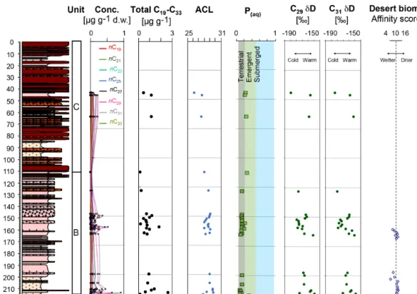
4.5 n-Alkane abundances andδD record

Evidence for hydroclimate-driven vegetation change in the Ejina Basin is provided from biomarker data (Fig. 9).

The short-chainnC19n-alkane is most abundant between core depths 64 to 44.1 m. Concentrations, however, are low and range between 0.048 and 0.068 µg (g dry weight)⁻¹ of sediment. Mid-chainn-alkanes such as nC₂₃–nC₂₅ can be found in samples between 217 to 44.1 m and have higher concentrations with a maximum value of 0.123 µg g⁻¹ dry weight occurring at 159.2 m depth. Long-chain n-alkanes nC₂₇–nC₃₃are dominant with a maximum value of 0.928 µg (g dry weight)⁻¹at 215.45 m core depth. We examineP_aq, which is a proxy ratio that highlights the terrestrial, emergent aquatic, and submerged aquatic macrophyte origins of the lipids (Ficken et al., 2000). With a few exceptions, much of the record has lowPaqvalues around 0.1, indicating that the n-alkanes likely originate from terrestrial rather than aquatic sources (Fig. 9).

TheδD values of long-chain terrestrially derived leaf-wax n-alkanes show a strong linear relationship to precipitation δD values across a wide range of environments (Sachse et al., 2004, 2012; Hou et al., 2008). In the nearby Quidam Basin, Koutsodendris et al. (2018) interpretedδD ofn-alkanes as sensitive recorders of palaeoclimatic variability, particularly sensitive indicators of temperature and moisture source variability (Gat, 1996; Sachse et al., 2012; Yao et al., 2013).

Here,δD measurements based on leaf-wax nC₂₉ andnC₃₁ alkanes yielded δD values between−189 ‰ and −148 ‰

(13)

G. Schwamborn et al.: Sediment history mirrors Pleistocene aridification 1387 and−184 ‰ and−148 ‰, respectively. TheδD wax values

from the nC₂₉ and thenC₃₁ alkanes are highly correlated (r²=0.95), which suggests a similar origin and is thought to be from terrestrial plants.

5 Discussion

Earth surface dynamics include a variety of processes that result in mixing of grain size subpopulations in sedimentary systems. Sediment from different sources can be transported and deposited by a multitude of sedimentological processes that have been linked to climate, vegetation, geological, and geomorphological dynamics as discussed in Dietze and Dietze (2019). The record from core GN200 has variable grain size distributions (Fig. 2c) indicating various transport processes that have shaped the depositional environment in the endorheic Ejina Basin. The interpreted endmembers fluvial, aeolian, playa (or sheetflood), and lacustrine processes have smooth transitions reflecting several energy regimes as is typical for desert and alluvial fan environments (Blair and McPherson, 1994). Only recently Yu et al. (2016) described alluvial gravels, fluvial sands, aeolian sand, sandy loess, and lacustrine clays as main sediment types that can be found in the Ejina Basin. Interpretations of nearby cored sediments (230 m long core D100) have related the coarse- grained portions – resembling EM 5 in GN200 – to high- energy fluvial transport from local areas such as the northern (Gobi Altay–Tien Shan range) and western (Beishan) catchment of the basin (Wünnemann et al., 2007b). Following this study, well-sorted fine sand as found in core D100 resembles EM 4 in GN200 and is likewise interpreted as being of aeolian to fluvial origin. Coarse and fine silt deposits resem- ble EM 3 and EM 2 and indicate playa-like depositional environments under different energy systems. Successions of finer to coarser silt layers building up much of unit B suggest that the depositional processes involved alternating hydrological conditions. Possibly this includes occasional desiccation events in the playa plain as is visible from individual layers of well-sorted fine sand, which suggest aeolian deposition at the site. The entire absence or very poor preservation of pollen in 41 out of 62 selected samples taken from a 57 m section, mainly representing this playa-like sedimentation environment, confirms our interpretation. On the other hand, bioindicators such as ostracods and gastropods docu- ment temporarily subaquatic conditions as are found in ponds and playa lakes. Ostracod communities are dominated byIly- ocypris sp., which prefers fresh- to brackish-water habitats (Mischke, 2001; Yan, 2017). A high abundance of ostracod valves can be evidence for short transport with a proximate burial (Mischke, 2001). Gastropods are represented byRadix peregra, which thrives in waters with a salt content of up to 33.5 ‰ (Verbrugge et al., 2012). This is also true for unit B sediments, which are interpreted to represent playa-lake environmental conditions.

Formation and transformation of clay minerals in soil pro- files and regoliths is determined by an interaction between the geology, drainage control by geomorphology, and the climate of the source terrain (Singer, 1984; Hillier, 1995; Wil- son, 1999; Dill, 2017). Tracking clay mineralogical changes in the detrital sedimentary compositions of the Ejina Basin by means of XRD data thus can aid the interpretation of environmental changes. Variations in the Ejina Basin clay mineralogy appear to be closely linked to main changes in depositional environments: mixed-layer clays characterize sediment layers belonging to the Red Clay formation (223.7–

222.6 m) and overlying deposits that have incorporated reworked portions of it (222.6–217.0 m) (unit A), smectite- rich clay characterizes the playa environment (large parts of unit B), and chlorite-rich clays are transported with Heihe river sediments (unit C with overlap to unit B).

Complementary detrital and authigenic signals of sediment origin are preserved in the bulk XRD and XRF data and can support the interpretation of sediment environments (e.g. Hillier, 2003; Jeong, 2008; Song et al., 2009). As with the clay signals the unit A sediments, which belong to the Red Clay formation, are well defined by XRD bulk data; i.e.

unit A is markedly dominated by quartz and feldspar when compared with unit B and unit C (Fig. 6).

SEM and XRD analyses of samples with higher concentrations of sulfur from nearby core D100 yielded evidence of gypsum formation when sulfur increased (Wünnemann et al., 2007a). It has been interpreted as pointing to a stepwise shrinkage of the water body under dry and warm conditions. Within the playa-lake succession in unit B prominent peaks of magnetic susceptibly along with sulfur likely indicate greigite (Fe₃S₄) formation (Fig. 5). Preservation of greigite can occur in terrigenous-rich and organic-poor sediments, and it is proposed to result from a dominance of reac- tive iron over organic matter and/or hydrogen sulfide, which otherwise would favour pyritization reactions (Blanchet et al., 2009). In fact, unit B sediments do not contain organic matter based on a set of TOC measurements using an elemental analyser, which produced results only below the detection limit of 0.1 % scattered over the unit (not displayed).

The record ofn-alkanes suggests large glacial and interglacial variability preserved in the record. The concentration and distribution ofn-alkanes allow for insight into the vegetation dynamics in the Ejina Basin and its catchment.

Plants produce a waxy coating on the surface of their leaves that protects them from desiccation (Eglinton and Hamil- ton, 1967). These waxes can be transported by wind or water to the sediments where they are robust over geologic timescales (Eglinton and Hamilton, 1967). While long carbon chain lengths are commonly more dominant in terrestrial higher plants (nC₂₇–nC₃₅), aquatic algae and microbes are often predominantly composed of shorter chain lengths (nC₁₇–nC₂₁) (Ficken et al., 2000). The mid-chain length homologues nC₂₃–nC₂₅ often produced in smaller quanti- ties by terrestrial higher plants, are often found in abun-

(14)

Figure 8.Percentage pollen diagram summarizing the results of pollen analysis presented in this study. The biome score calculation of the dominant desert biome uses the approach and pollen taxa to biome attribution described in Herzschuh et al. (2004).

Figure 9.GN200 core with concentrations ofn-alkanes (d.w.=dry weight) and average chain length (ACL); coloured areas highlight the interpretation of lipid origin (based on Ficken et al., 2000) andδD values with palaeoclimate interpretations versus depth. The desert biome record from Fig. 8 is repeated for comparison.

(15)

G. Schwamborn et al.: Sediment history mirrors Pleistocene aridification 1389 dance in aquatic macrophytes (Cranwell, 1984; Ficken et

al., 2000).The discontinuous GN200 biomarker record re- veals several intervals where glacial-to-interglacial changes are preserved: between 217 to 210 m a change from glacial to interglacial conditions and between 165 to 148 m a cycle from interglacial to glacial and back to interglacial conditions. Samples further upcore suggest both glacial (128, 44 m) and interglacial (64, 46 m) conditions. GN200 δD values range between −145 ‰ (interglacial) and −190 ‰ (glacial). Considering that the Ejina Basin is located in the mid-latitudes of the Northern Hemisphere and exhibits strong seasonal temperature variability, we interpret leaf-wax δD values in GN200 as primarily a measure of temperature and indicative of the origin of moisture following interpretations given in Koutsodendris et al. (2018). As such, on glacial–interglacial timescales, more negativeδD wax values should reflect colder rather than wetter conditions and/or a more distant water source. Koutsodendris et al. (2018) further propose that the δD value of nC₂₉ and nC₃₁ alkanes can be affected by evaporative deuterium enrichment of leaf water caused by enhanced evapotranspiration under low at- mospheric humidity based on Sachse et al. (2006), Seki et al. (2011), and Rach et al. (2014). In this way, GN200 samples from dry glacials can be also affected by evapotranspiration.

The fossil pollen spectra composition resembles modern pollen spectra from the Alashan Plateau, collected from a landscape covered with shrubby desert vegetation consisting of Chenopodiaceae, Nitraria, andEphedra species (Herzschuh et al., 2004). Discontinuous pollen data from 217–207 m indicate that shrub desert vegetation with pre- dominance of Chenopodiaceae andEphedra grew close to the coring site, and that mountain forests south of the coring site occupied a smaller area between 2.523 and 2.410 Ma.

This correlates relatively well (within the error of the age model) with the long phase of low precipitation and tun- dra dominance in the Lake El’gygytgyn record from north- east Asia (Brigham-Grette et al., 2013; Tarasov et al., 2013).

The fact that our pollen record does not reflect changes from glacial to interglacial conditions between 217 to 210 m, as indicated by the biomarker record, may suggest that vegetation and pollen records from the arid region primarily mirror moisture conditions and not the temperature signal, as interpreted here forδD. The observed changes in the pollen composition between 203–197 m (2.363 to 2.294 Ma) suggest a transition from an arid shrubby desert environment similar to the previous interval to a less arid one. The pollen composition indicates a further decrease in the climate aridity and spread of the temperate zone mountain forest in the upper reaches of the Heihe at 193 m (2.249 Ma) In the interval 168–160 m (1.954–1.857 Ma) higher pollen concentrations in the record are associated with a greater role for chenopods (known as very high pollen producers) in regional vegetation, indicating an increase in aridity (Herzschuh et al., 2004; Hou, 2001).

In contrast to a former chronology from drilling into the Ejina Basin (i.e. 230 m long core D100, Wünnemann et al., 2007a), where a palaeomagnetic dataset has been interpreted to encompass 250 ka, the playa-lake environment is now interpreted to extend further back in time. The onset of more humid conditions with lake sedimentation must date back to the early Pleistocene (> 2 Ma) based on the Brun- hes/Matuyama chron boundary at 60 m core depth and the occurrence of the Jaramillo and Olduvai sub-chrons interpreted in this study (Figs. 3 and 4). A further linear extrapolation of the time axis down to the core bottom is based on the following assumptions: (i) the Gauss chron (normal polarity) is not detected in the record; thus, GN200 reaches the onset of the Matuyama chron at maximum (2.59 Ma). Between 222.6 and 223.7 m a reversal to normal (Gauss?) is indicated but statistically not significant. But the extrapolated value comes close to the assumed value from linear extrapolation.

(ii) The depositional sequence does not change prominently;

the core portion between 222.6–172.0 m has an alternation of fluvial–alluvial layers intercalating with playa-lacustrine sediments typical for desert environments. In this sense, the two upper radionuclide ages (> 2 Ma) are reversals (Fig. 4), which can be explained by reworking of old material that has been eroded and transported from the catchment prior to its final deposition in the Ejina Basin. In contrast, the lower sample age at 53.1 m depth (0.84±0.12 Ma) is accepted as supporting the palaeomagnetic depth-to-age distribution because of its approximate overlap with it. (iii) Unit A sediments (222.6–217.0 m) are interpreted to be reworked material from the underlying Red Clay formation implying that the Neogene likely is close below the core bottom. (iv) Pos- sibly there is a hiatus between the lowermost layers (223.7–

222.6 m) and the overlying sediments (< 222.6 m); the core bottom (223.7–222.6 m) consists of fanglomerate sediments and red-coloured medium sandy sediments that are interpreted to represent the Red Clay formation, whereas sediments above a sharp boundary at 222.6 m turn into grey- coloured fine sand to silt layers. The transition from an oxic to an anoxic environment is distinct.

The resulting linear depth-to-age relationship suggests that on a Quaternary timescale the overall sedimentation rates in the Ejina Basin are fairly constant. This matches results from Willenbring and von Blanckenburg (2010), who show that during the Late Cenozoic global erosion rates and weather- ing are stable; thus demonstrating that erosion and accumulation rates are balanced on mega-annum timescales. Even though at smaller scales one may distinguish between inde- pendent histories at the subcontinental and basin scales, our age model accepts that extrusion and crustal shortening are complementary processes that have been successively dominant throughout the India–Eurasia collision history (Mé- tivier et al., 1999). This is thought to also affect the Ejina Basin sediment history, which receives detritus from the Qil- ian Shan in the northern Tibetan upland. On long timescales (Ma) the sedimentation rates in the Ejina Basin are low, i.e.