Absent–minded drivers in the lab: Testing Gilboa’s model
¤Ste¤en Hucky Royal Holloway
Wieland Müllerz Humboldt University June 20, 2000
Abstract
This note contributes to the discussion of decision problems with imperfect recall from an empirical point of view. We argue that, using standard methods of exper- imental economics, it is impossible to induce (or control for) absent–mindedness of subjects. Nevertheless, it is possible to test Gilboa’s (1997) agent–based approach to games with imperfect recall. We implement his model of the absent–minded driver problem in an experiment and …nd, if subjects are repeatedly randomly rematched, strong support for the equilibrium prediction which coincides with Pic- cione and Rubinstein’s (1997) ex ante solution of the driver’s problem.
Keywords: imperfect recall, the absent-minded driver’s paradox, experiments.
JEL classi…cation numbers: C72, C92.
1 Introduction
In a provocative paper Piccione and Rubinstein (1997a, henceforth P&R) reinstated the topic of imperfect recall on the agenda of game theory. The response to their paper was overwhelming and led to a special issue of Games and Economic Behavior containing next to P&R’s paper several responses and discussions by eminent theorists.1
¤We thank Jörg Oechssler for helpful comments.
yDepartment of Economics, Royal Holloway, Egham, Surrey TW20 OEX, UK, Fax: +44 1784 439534, e-mail: S.Huck@rhbnc.ac.uk.
zDepartment of Economics, Spandauer Str. 1, 10178 Berlin, Germany, Fax +49 30 2093 5704, email:
wmueller@wiwi.hu–berlin.de.
1Games and Economic Behavior, Vol. 20, No.1, 1997.
There was, however, one question neither of these papers (and none of those that were published at other places) addressed—the question of whether and how models of imperfect recall can be tested. This note o¤ers a …rst investigation into this matter and provides data from an experimental study.
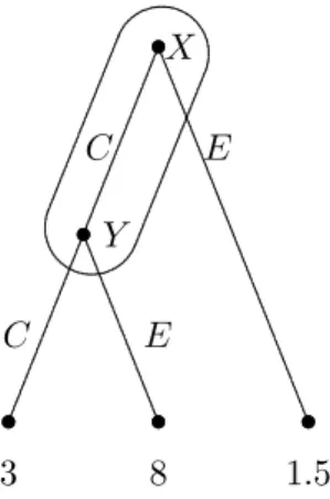
Much of the theoretical discussion focussed on a toy game with which P&R in- troduced their treatment of imperfect recall, the absent–minded driver game. The absent–minded driver starts his journey at node X where he can eitherexit orcontinue to Y where he faces the same choice. The payo¤s (as given in Figure 1) are 1.5 after exiting at X, 8 after exiting at Y and 3 after continuing at Y.
...
...
...
...
...
...
...
...
...
...
...
...
...
...............
............
.....................
............
.........
...
...
...
...
...
...
...
...
...
...
...
...
...
............
...............
......
C E
C E
3 8 1:5
.....................
...
.....................
...
...
...
...
...
...
...
...
...
...
...
...
...
...
...
...
...
...
...
...
...
...
ss
ss
ss ss
ss
X
Y
Figure 1: The absent-minded driver problem
The driver su¤ers from imperfect recall insofar as he cannot distinguish between X and Y, i.e., he cannot remember whether he already passed one of the nodes. P&R claimed that the driver were facing a paradoxical problem. They argued that the driver’s reasoning before he starts his journey (the “planning stage”) were inconsistent with his reasoning once he reaches a decision node (the “action stage”). Others did not share P&R’s view. In the same issue Aumann, Hart and Perry (1997, henceforth AH&P), for example, let the paradox disappear by observing that the driver can only control hiscurrent action while considering the rest of his play as…xed. P&R assumed that the driver, deciding at one node about a probability with which to exit, can simultaneously control his behavior at the other node and they defended this view—as
one among many reasonable approaches—in their synthesis (Piccione and Rubinstein 1997b) that appeared at the end of the special issue.
In this note we do not want to go into further detail about the theoretical contro- versy. Rather we want to explore whether and howany theoretical prediction for the problem at hand can be empirically tested. As it turns out “whether and how?” cannot be easily answered.
Usually, it is more or less straightforward to implement a game in an experimental environment. So why not the absent–minded driver game? The answer is that exactly the same feature that makes it theoretically interesting also makes it (almost) impossible to implement. Experimenters cannot induce imperfect recall of subjects. That is, at least experiments adhering to the standard rules and procedures of experimental economics.
Of course, one could think about deceiving subjects or perhaps about narcotizing them without their prior consent. In fact, we are convinced that the latter would certainly do the trick. Alas, we prefer not to.
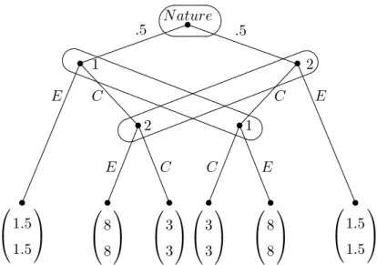
Nevertheless we did test an absent–minded driver model, namely the one suggested by Gilboa (1997, also in the special issue). Gilboa argued, somewhat similar to AH&P, that the correct modeling approach to the problem would be to assume two identical agents of the driver, who each only face one decision node along a path. More speci…- cally, he assumes the structure shown in Figure 2. There are two agents, 1 and 2. The
…rst move is by nature deciding (with equal probabilities) which of the two agents will decide at the …rst decision node. Then, if necessary, nature calls the other agent upon to act at the second decision node. Since both agents represent the same driver, they receive at each terminal node the same payo¤s. And though modeling a situation of imperfect recall, the game itself is one of perfect recall.
As Gilboa shows this approach lets P&R’s inconsistency disappear. The game has a unique symmetric equilibrium in which the agents choose the same probabilities for exit as P&R’s driver would before starting his journey (in the “planning stage”). There are, however, two further asymmetric equilibria of this game. But Gilboa (p.29) argues:
“Since we have a compelling theoretical reason to focus on symmetric equilibria, we should simply do so.”
..
....
..
....
....
..
....
....
..
....
..
....
....
..
....
....
....
..
....
....
..
....
....
..
....
....
..
....
....
..
....
....
..
....
....
..
....
....
....
..
....
....
..
....
....
..
....
....
..
....
..
....
....
....
..
....
....
..
....
....
..
....
....
..
..................
Nature
:5 ..................................................... :5
....................................................
...
...
..................
............
...
...
...
...
...
...
...
...
...
...
...
...
...
...
...
...
...
...
...
...
...
...
1
E C
0
@1:5 1:5
1 A
...
...
...
...
...
...
...
...
...
...
...
...
...
...............
............
......
ss ss
2
E C
0
@8 8
1 A
0
@3 3
1 A ss
ss
ss
......
......
........
.......
.......
........
.......
....
.......
.......
........
.......
........
.......
.......
........
.......
.......
........
.......
........
.......
.
......
...............
..................
...............
............
2
C E
...
...
...
...
...
...
...
...
...
...
...
...
...
...............
............
......
ss ss
1
C E
0
@3 3
1 A
0
@8 8
1 A
0
@1:5 1:5
1 A ss
ss
ss
....
....
..
......
.......
............
................................
..................................
...............................
..
..
..
....
..
..
....
....
....
......
...
...
.........
..............................
..
....
..
..
..
....
.
............................................................
............................................................
ss
Figure 2: The agent–based version of the absent–minded driver problem To some extent, our study examines the (empirical) legitimacy of this view.2 Our main …nding is that it appears indeed legitimate—provided that subjects (a) have time to learn and (b) are constantly rematched with di¤erent partners. If they are not, i.e., if they play Gilboa’s game with the same partner over and over again, they eventually learn to coordinate their actions on one of the Pareto–superior asymmetric equilibria.
The remainder of the paper is organized as follows. Section 2 presents theory and the experimental design. The results of the experiments are reported in Section 3 and Section 4 concludes.
2 Theory and experimental design
Our experiment is based on the game in Figure 2. This game has two asymmetric Nash equilibria in pure strategies, namely (E; C) and (C; E): They are supported by the following beliefs: Whereas the agent playingE believes with equal probability to be at
2Note that Binmore (1997)—although appreciating the result to which Gilboa’s approach leads—
casts doubts on the appropriateness of “modeling players as teams of agents with identical preferences”
(p.60). He argues ”that the right way or ways to proceed will remain mysterious until we have satis- factoryalgorithmic models of the players we study” (p.61). However, as argued above, we think that Gilboa’s approach to games with imperfect recall seems to be the only one that can be tested in the lab.
each node in his information set, the agent playing C believes with certainty to be at the node following nature’s move. In addition, the game has a symmetric equilibrium in mixed strategies in which both agents play E with probability :35which is also the ex ante optimal strategy for a single player (at “the planning stage”) in P&R’s game with accordingly modi…ed payo¤s. For each agent the symmetric equilibrium is supported by the belief to be with probability20=33at the node following nature’s move.3 Whereas the expected payo¤ for both players is 4:75in the asymmetric equilibria, it is3:6125in the symmetric equilibrium.
The experiments were computerized4 and conducted at Humboldt University from October 1999 to January 2000. Subjects were students of economics or business admin- istration. Upon arrival in the lab they were assigned a computer screen and received written instructions. After reading them, questions could be asked which were answered privately. There were two treatments. In treatment Fix subjects were once matched in pairs and then interacted repeatedly. In treatment Rand subjects were (in groups of six) randomly rematched in each period. Both treatments lasted over 60 periods.
Whereas in the former treatment 20 subjects participated, we conducted six sessions for the latter treatment. Thus, altogether 56 subjects participated in the experiments.
The number of periods to be played was known in both treatments.
In the instructions (see Appendix A) subjects were informed that they (and another subject with whom they are matched) had to decide between two options: the option to go “left” and the option to go “right”. The computer would then—with equal probability—decide who were to move …rst. The payo¤ consequences of the decisions were explained both graphically and verbally (see Appendix A). Subjects were informed, however, that they had to choose between left and right without knowing whether they will go …rst or second.
Furthermore, subjects were told that each of the 60 periods would consist of 100 rounds. In each period they would have to makeone decision governing their behavior inall 100 rounds. Basically, this allowed us to elicit mixed strategies in a rather natural way. Subjects were asked to imagine an urn with 100 balls. They were told that they
3Given the agents mixed strategies and using Bayes’ rule, agent 1’s conditional probability to be at the node following the move by nature equals :5+:5£:65:5 =2033:
4We used the software tool kitz-Tree, developed by Fischbacher (1999).
could determine the composition of the urn, i.e., how many of the balls would represent
“going to the left” and how many “going to the right”. Once the composition of the urn was decided, the urn would be relevant for 100 runs. The instructions then explained how these runs would be carried out by the computer (see Appendix A for details).
At the beginning of each period, subjects were asked to enter their mixture of left and right balls into two boxes (see the top panel in Figure 4 in Appendix B which shows the decision screen).
At the end of a period, subjects were informed about: (i) how many times they went …rst respectively second in this period; (ii) for each of these two cases, how many times they earned respectively 1.5, 3, or 8 points (along with the relative frequencies of these cases); and (iii) the payo¤ in this period and the accumulated payo¤ so far (see the bottom panel in Figure 4 in Appendix B which shows an information screen.)
Subjects were informed that the sum of all pro…ts accumulated during the 6.000 rounds (60 periods with 100 rounds) would determine their …nal monetary payo¤. The exchange rate was Points 900 = DM 1. Average earnings in treatment Fix (which lasted for about 50 minutes) were DM25:50 and DM24:30in treatment Rand(which lasted for about 70 minutes).
3 Results
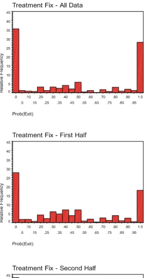
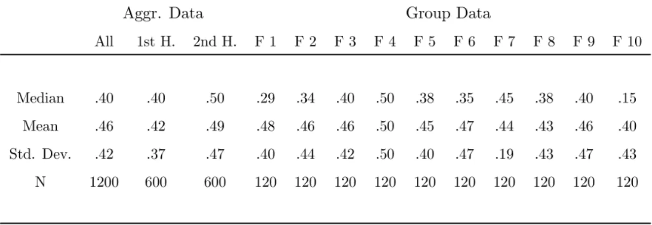
Figure 3 displays the distribution of probabilities with which E(xit) was chosen. On the left– (right–) hand side the results of treatment Fix (Rand) are shown. On each side, the top panel shows the choices across all periods and the middle (bottom) panel the choices in the …rst (second) half of the experiment (in each case aggregated over all groups). Tables 1 and 2 report summary statistics of the two treatments both on the aggregate (all data, …rst and second half) and the group level.
Let us …rst consider treatmentFix. As shown in Table 1, the median of prob(E)–
choices equals .40 for all data and increases from .40 in the …rst half to .50 in the second half. The mean equals .46 for all data and increases from .42 in the …rst half to .49 in the second half. This clear change over time is corroborated by comparing the distribution of choices in the second half of the experiment with the one in the …rst half.
Figure 3: Frequency distribution (Left: TreatmentFix; Right: TreatmentRand)
Aggr. Data Group Data
All 1st H. 2nd H. F 1 F 2 F 3 F 4 F 5 F 6 F 7 F 8 F 9 F 10
Median .40 .40 .50 .29 .34 .40 .50 .38 .35 .45 .38 .40 .15
Mean .46 .42 .49 .48 .46 .46 .50 .45 .47 .44 .43 .46 .40
Std. Dev. .42 .37 .47 .40 .44 .42 .50 .40 .47 .19 .43 .47 .43
N 1200 600 600 120 120 120 120 120 120 120 120 120 120
Table 1: Summary statistics of Treatment Fix
Means and medians, however, only tell half the story as can be seen in Figure 3. The most important feature of the data is that the frequency of the pure–strategy choices (and choices very close to .0 and 1:0) increases over time. Whereas the choice of the strategies in these two categories5 count for 45:5 % of all cases in the …rst half, they count for 81:3 % of all cases in the second half of the experiment. In fact, …ve groups in treatment Fixreach perfect coordination on an asymmetric equilibrium. Whereas one of these groups is—surprisingly—coordinated from the very start, the other groups need some more time and are coordinated by the end of period 30. Four further groups are eventually very close to perfect coordination. Only one of the 10 groups does not manage to coordinate its actions. We summarize this in
Result 1 When subjects play Gilboa’s game repeatedly with the same partner they (almost always) manage to coordinate themselves on one of the Pareto–optimal asymmetric equilibria.
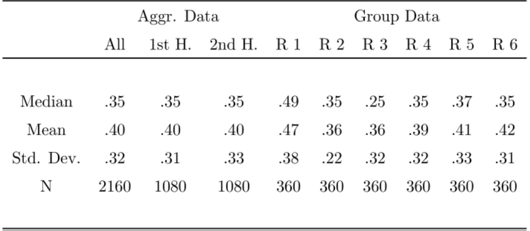
Next consider treatment Rand. Strikingly, the median of prob(E)–choices across all groups equals exactly the equilibrium probability of .35 in both halves of the ex- periment! (See Table 2.) The mean equals .40 without changing much over time.6 The equilibrium prediction also does well against average observed data of individual groups. As can be seen from Table 2, the median is equal (or very close to) .35 in
5For categories 0 and 1.0 we included choices in the interval [.0, .025) and [.975, 1.0] respectively.
6Note that, due to the bounded strategy space, one would expect the mean to exceed the median with most random error models.
Aggr. Data Group Data
All 1st H. 2nd H. R 1 R 2 R 3 R 4 R 5 R 6
Median .35 .35 .35 .49 .35 .25 .35 .37 .35
Mean .40 .40 .40 .47 .36 .36 .39 .41 .42
Std. Dev. .32 .31 .33 .38 .22 .32 .32 .33 .31
N 2160 1080 1080 360 360 360 360 360 360
Table 2: Summary statistics of TreatmentRand
four of the six groups. Inspecting the distributions of choices (Figure 3) we do not …nd much of a time trend. The …ndings for treatment Rand are summarized in
Result 2 When subjects play Gilboa’s game repeatedly with randomly matched part- ners the symmetric mixed equilibrium predicts aggregate behavior very well.
4 Conclusion
This note contributes to the discussion of decision problems with imperfect recall from an empirical point of view. We argue that, using standard methods of experimental economics, it is impossible to induce (or control for) absent–mindedness of subjects.
Thus, even the simple absent–minded driver game, as originally introduced by Piccione and Rubinstein (1997a), cannot be directly tested. Hence, the theoretical dispute about how such games should be treated remains a theoretical dispute. Regardless, which predictions are made they cannot be falsi…ed.
However, Gilboa’s (1997) approach to problems with imperfect recall, which splits the decision maker into two (or more) identical agents, is genuinely testable. In some sense, this might also be seen as an advantage his approach has over others. Moreover, we …nd that the symmetric equilibrium prediction he emphasizes is strikingly accurate—
provided that subjects act in an environment that resembles the one–shot nature of the theoretical model and also gives opportunities for learning. In case of repeated
interaction we …nd, however, that most subjects eventually manage to coordinate on one of the Pareto–superior asymmetric equilibria.
The question which of the two treatments captures the theoretical problem more accurately is ambiguous. On the one hand, one might argue that the random-matching treatment is more accurate as it re‡ects the one-shot nature of the game. On the other hand, the …xed-pairs treatment might be more appropriate with respect to the multiple-selves interpretation. (The other selves I am playing with in reality always remain identical.)
Nevertheless, we conclude that the modelling approach suggested by Gilboa allows to make testable and—in the light of the result with random matching—reliable pre- dictions.
References
[1] Aumann, R. J., S. Hart, and M. Perry (1997): The absent–minded driver, Games and Economic Behavior 20, 102-116.
[2] Binmore, K. (1997): A note on imperfect recall, in: Understanding Strategic Inter- action: Essays in Honor of Reinhard Selten, eds.: Albers, W., Güth, W., Hammer- stein, P., Molduvanu, B., and Van Damme, E., 51-62, Springer-Verlag.
[3] Fischbacher, U. (1999): Z-Tree, Zurich toolbox for readymade economic experi- ments,Working paper Nr. 21, Institute for Empirical Research in Economics, Uni- versity of Zurich.
[4] Gilboa, I. (1997): A comment on the absent–minded driver paradox, Games and Economic Behavior 20, 25-30.
[5] Piccione, M., and A. Rubinstein (1997a): On the interpretation of decision problems with imperfect recall,Games and Economic Behavior 20, 3-24.
[6] Piccione, M., and A. Rubinstein (1997b): The absent–minded driver’s paradox:
Synthesis and responses,Games and Economic Behavior 20, 121-130.
Appendix
A Translated instructions of treatment Fix
Please read these instructions carefully! Do not speak to your neighbors and keep quiet during the entire experiment! In case you have questions give notice. We will then come to your place.
In our experiment you will repeatedly make a decision. By doing that you can earn money. How much money you will earn depends on your decision and on the decisions made by another participant you are matched with. All participants have identical instructions. The situation in which you have to decide is simple.
You and the other participant you are matched with must choose between two options: the option to go “left” and the option to go “right”. Then it will be randomly decided who of you goes …rst. The following picture illustrates how many points you can earn depending on what happens.
1
2
1,5 Left
Left Right
Right
² If the one who goes …rst (in the picture denoted by “1”) decided to go left, both of you get 1.5 points.
² If the one who goes …rst decided to go right then it depends on what the other (in the picture denoted by “2”) did:
– If he decided to go left, both of you get 8 points.
– If he also decided to go right, both of you get 3 points.
(Thus, both of you always get the same number of points.)
The problem, however, is that when you have to decide between “left” and “right”, you don’t know whether you go …rst or second. This will be randomly determinedafter you have decided. The odds are 50:50.
So far the main rules. Now the exact procedure.
Each of 60 periods will consist of 100 rounds in which the situation will be carried out once. In each period you decide as follows. Imagine an urn with 100 balls. You can determine how many of these balls stand for “going to the left” and “going to the right”. In each run the computer randomly decides who of you goes …rst. Of the chosen participant the computer then randomly draws one ball from the urn (and puts it back afterward). If it is a ball showing “left” then this round stops and both participants get 1.5 points. In case the ball shows “right” then the computer also chooses a ball from the urn of the other participant. Depending on what kind of ball it is you get payo¤s as described above.
This procedure makes it possible for you not to do always the same in the 100 rounds (within one period). However, if you always want to do the same, you can do that by providing your urn only with “left” or “right” balls. If on the other hand you want to go on average “so and so often” to the left or to the right, respectively, you can do that by a mixture of “so and so many” left and right balls.
Please keep the following in mind: Since in each round chance decides, it can happen that you go …rst in less than 50 rounds. Furthermore, it can happen, that you go left (or right) more often than the number of Left balls (Right balls) you put in the urn.
On the Screen you will see two boxes (one for left one for right). In each of them you will enter a number. The sum of the numbers must be 100.
At the end of a period, you will get to know what happened in the 100 rounds of this period. Thereby you will get to know how many points you have earned. Then a new period starts which will be conducted following the same rules as the …rst. Altogether there will be sixty such periods.
The sum of your points you earned in the 6.000 rounds (60 periods times 100 rounds) determine your payo¤ in DM. Here you get 1 DM for every 900 points immediately after the experiment.
B Screen shots
Figure 4: English translation of a decision screen (above) and an information screen (below)