presented by
Diplom-Physiker Peter Schuller
born in Bucharest
Oral examination: 16th October 2002
Referees: Prof. Dr. Christoph Leinert Prof. Dr. Wolfgang Duschl
For calibration of the instrument during observations, calibrator stars are used. As part of the selection process of suitable objects for a database of such stars, a sub-sample of candidates was checked by interferometric observations in the K0 band (2.0. . . 2.3µm). Special attention was payed to differential effects in narrow sub-bands.
The potential of stellar interferometry is shown in the case of some late type stars. High spatial resolution data were used to constrain model parameters of the circumstellar envelopes of these objects.
Zusammenfassung
Kalibration von MIDI, dem Mittelinfrarot-Interferometer f¨ur das VLTI DasMIDI-Instrument (MID-infrared Interferometric Instrument) wird amVLTI(Very Large Telescope Interferometer) stellare Langbasisinterferometrie im N-Band (8. . . 13µm) durchf¨uhren.
Im Vorfeld des Aufbaus von MIDI waren einige vorbereitende Aufgaben zu l¨osen, die die Kalibrie- rung des Instruments im Labor betrafen. Die interne Verz¨ogerungsstrecke, die eine wesentliche Untereinheit von MIDI darstellt, wurde sorgf¨altig getestet, um Aussagen ¨uber deren G¨ute zu treffen. Lichtquellen f¨ur verschiedene Zwecke wurden bereitgestellt und mit geeigneten Optiken versehen. Spektrale Referenzen wurden ebenfalls einbezogen. Die Wechselbeziehung zwischen einer kalibrierten Verz¨ogerungsstrecke und spektraler Kalibration wird aufgezeigt.
Zur Kalibration des Instruments w¨ahrend der Beobachtung werden Kalibratorsterne benutzt.
Als Teil des Auswahlverfahrens von geeigneten Objekten f¨ur eine Datenbank von solchen Ster- nen wurde eine Auswahl von Kandidaten durch interferometrische Beobachtungen im K0-Band (2.0. . . 2.3µm) ¨uberpr¨uft. Besonderes Augenmerk wurde dabei auf unterschiedliches Verhalten in schmalen Teilb¨andern gelegt.
Die M¨oglichkeiten stellarer Interferometrie werden am Beispiel einiger Sterne sp¨aten Types aufgezeigt. Daten mit hoher r¨aumlicher Aufl¨osung wurden benutzt, um Modellparameter der zirkumstellaren H¨ullen dieser Objekte einzugrenzen.
2.2.1 General Case . . . 9
2.2.2 Uniform Disk . . . 10
2.2.3 Effect of a Finite Bandwidth . . . 11
2.3 Discussion . . . 11
2.4 A Simple Visibility Measuring Algorithm . . . 13
3 MIDI at the VLTI 17 3.1 The VLTI Environment . . . 17
3.1.1 Telescopes . . . 17
3.1.2 Delay Lines . . . 19
3.1.3 Interferometric Instrumentation . . . 21
3.2 Mid-Infrared Interferometry with MIDI . . . 24
3.2.1 Scientific motivation . . . 24
3.2.2 Technical Aspects . . . 24
3.2.3 Atmospheric Conditions . . . 25
3.3 The MIDI Instrument . . . 27
3.3.1 Warm Optics . . . 27
3.3.2 Dewar . . . 29
3.3.3 Cold Optics . . . 29
4 Calibrations 33 4.1 Overview . . . 33
4.2 Performance of Optical Path Length Modulators in MIDI . . . 34
4.2.1 Overview . . . 34
4.2.2 Results . . . 35
4.2.3 Discussion . . . 42
4.3 Calibration Light Sources . . . 43
4.3.1 The Monochromatic Source . . . 43
4.3.2 The Polychromatic Unresolved Source . . . 48
5.1 Calibrator Stars . . . 59
5.1.1 Overview . . . 59
5.1.2 Establishing a Database . . . 60
5.1.3 Interferometric Verification . . . 61
5.2 Interferometric Data and Astrophysical Modeling . . . 68
5.2.1 The Modeling Code . . . 68
5.2.2 Observational Data . . . 69
5.2.3 Comparison between Model and Observations . . . 69
5.2.4 Discussion . . . 70
6 Conclusion 77 A Signal Estimates 79 A.1 Limiting Magnitude for MIDI . . . 79
A.2 Radiation Sources and Detector Response . . . 83
A.2.1 Laser Sources . . . 83
A.2.2 VLTI Background . . . 85
A.3 Average Flux Density Versus Peak Intensity . . . 85
A.3.1 Gaussian Profile . . . 86
A.3.2 Circular Aperture . . . 86
B Retrieving Visibilities by Long Scan Fourier Analysis 89 B.1 General Description . . . 89
B.2 Data Analysis . . . 90
C Alignment of Calibration Sources 93 C.1 CO2 Laser . . . 93
C.2 Laser Diode . . . 96
C.3 Broad Band Source . . . 98
Bibliography 101 Abbreviations and Acronyms 107 At the end / Zum Schluß ... 109
3.2 VLTI optical train . . . 20
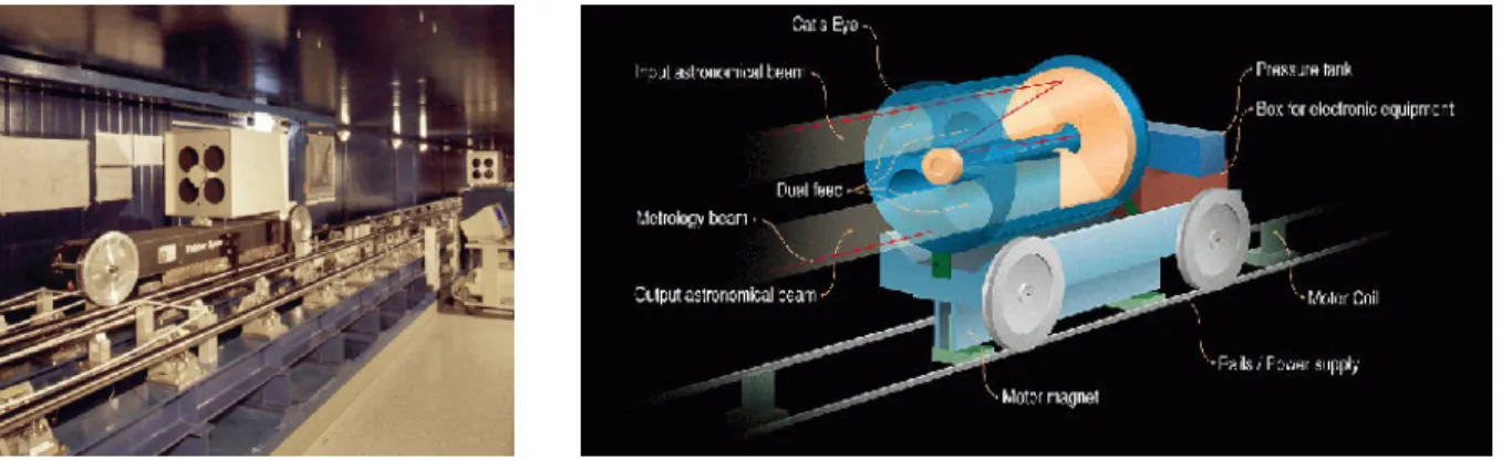
3.3 One of the VLTI Delay Lines . . . 21
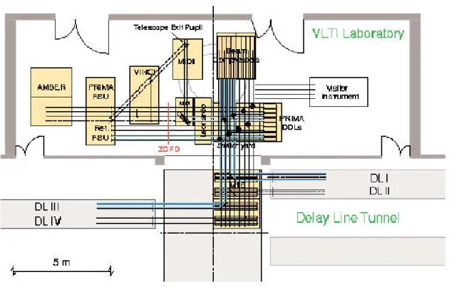
3.4 Ground plan of VLTI Interferometric Laboratory . . . 22
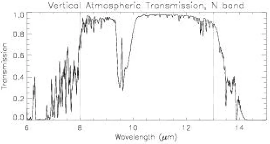
3.5 Atmospheric transmission in the N band . . . 25
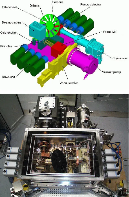
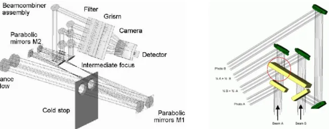
3.6 Scheme and overview of MIDI . . . 28
3.7 MIDI Dewar . . . 30
3.8 MIDI Cold Optics . . . 31
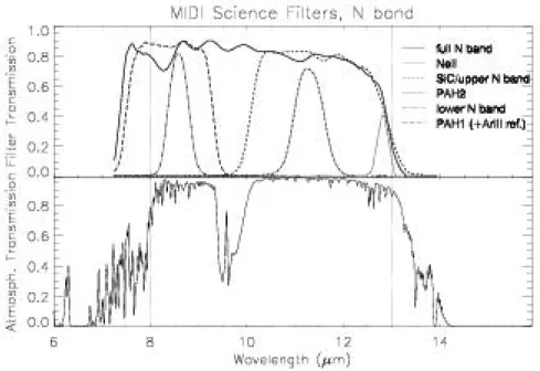
3.9 Science filters in MIDI . . . 32
4.1 Piezo stage and electronics . . . 34
4.2 Piezo test setup with HeNe interferometer . . . 35
4.3 Input signal for piezo tests . . . 36
4.4 Piezo response . . . 36
4.5 Residuals after fit of response . . . 37
4.6 Verification of piezo tests . . . 38
4.7 Noise and its spectrum of a piezo stage . . . 39
4.8 Stepping scanning mode . . . 40
4.9 Step response of the piezo . . . 40
4.10 Fourier scanning mode . . . 41
4.11 Fourier mode residual . . . 41
4.12 Tip-tilt angle of piezos . . . 42
4.13 CO2 laser with attenuation . . . 44
4.14 Laser diode system . . . 47
4.15 Laser diode wavelength . . . 48
4.16 Broad-band source with collimating optics . . . 49
4.17 PulsIR measurements at constant wavelength . . . 50
4.18 Detector images of broad-band interference . . . 51
4.19 Foil reference spectra . . . 52
4.20 Foil spectrum taken with MIDI . . . 53 iii
5.2 Measurements in narrow K filters onMIDI Calibrator Candidates . . . 64
5.3 Model output for α Ori . . . 71
5.4 Model output for R Leo, initial parameters . . . 72
5.5 Model output for R Leo, modified parameters . . . 73
5.6 Model output for SW Vir . . . 74
C.1 CO2 laser and attenuating optics . . . 94
C.2 Alignment of laser diode collimation paraboloid . . . 97
C.3 Broad band source . . . 98
C.4 Optical details of elliptical mirror . . . 99
5.1 Visibilities measured in K0 on MIDI Calibrator Candidates . . . 62
5.2 K band filters available with the FLUOR instrument . . . 63
5.3 Objects observed in spring 2002 with narrow K band filters . . . 65
5.4 Visibilities in narrow K filters measured on MIDI Calibrator Candidates . . . 65
5.5 Basic data of modeled objects . . . 69
5.6 Parameters used for modeling . . . 69
A.1 Limiting magnitude calculation . . . 82
v
spatial resolution. Up to the beginning of the seventeenth century, mechanical devices like sextants were used to measure positions on the sky. Representative of this era, one might name Tycho Brahe (1546 - 1601) who developed his well-known mural quadrant and performed some of the most precise and substantial astronomical observations of his time. A big step forward in observational techniques was initiated when optical devices were used for astronomical purpose for the first time. This fundamental change in instrumentation is usually associated with the name of Galileo Galilei (1564 - 1642). In 1609, he applied strong improvements to prototype telescopes originally invented in the Netherlands1. It was up toJohannes Kepler (1571 - 1630) to penetrate both the astronomical observations and the new technique with theory and thorough calculations, leading to the three Kepler Laws and a comprehensive treatment of the optics known at that time. This triumvirate might be regarded as prototypical for a fruitful linkage of instrumentation, observation, and theory in astronomy.
Ever since, telescopes have been improved and grown in size in order to see increasingly resolved details on the sky. However, every enlargement of the optics and mechanics involved had to be traded for technical feasibility that was and is possible at a time. And still for a long time stars remained unresolved. Yet, in 1868 Armand Fizeau (1819 - 1896) suggested an interferometric method to measure stellar diameters by placing a mask with two holes in front of a telescope’s aperture (Fizeau,1868). He had calculated that the resulting interferometric fringes would vanish at a separation related to the size of the star. The first successful application of interferometry to astronomy was performed by Albert Michelson (1852 - 1931) in 1891 by measuring the diameter of Jovian moons (Michelson,1891). Not until 1920 did Michelson also apply this method to stars which revealed for the first time the angular and, knowing its parallax, the linear diameter of a giant star (Michelson and Pease, 1921). For these measurements, Michelson used a setup that would become a major principle for modern stellar interferometry.
On a very rigid bearing construction fixed to the aperture of the largest available telescope, he placed two independent mirrors at a distance exceeding the telescope’s diameter. Their light was combined at a point where the paths of the produced beams were well matched, i.e., in
1There are, though, earlier reports of stellar observations in 1608, made mainly out of curiosity by Dutch lens makers. The first lunar drawings appeared in England made byThomas Harriot in summer 1609 (Helden,1995).
not suffer from the difficulties governing optical interferometry. Interferometry at radio wave- lengths is a well-established technique and presently an active area of research (Thompson et al., 2001;Finley and Goss,2000). Likewise, the technique of intensity interferometry was developed and demonstrated at optical wavelengths, using for the first time two independent telescopes (Hanbury Brown and Twiss, 1956b,a). Compared with Michelson’s amplitude interferometer this technique had the advantages of being less demanding in mechanical respect and of being essentially unaffected by seeing, i.e., moving and spreading of a star’s image due to atmospheric turbulence.
Then in the 1970s it was demonstrated that the technological demands on mechanical stabil- ity, which is necessary for performing Michelson’s experiment with two separate telescopes, had become solvable (Labeyrie, 1975). With this kind of interferometer a sensitivity much higher than with an intensity interferometer was obtainable. Starting in the 1970s, a number of op- tical interferometers were established, using different techniques of beam combination. Today, there are several long baseline stellar interferometers in operation mainly working at visible and near-infrared wavelengths (CHARA, COAST, GI2T, IOTA, NPOI, PTI, SUSI; see L´ena and Quirrenbach (2000), Session 3, for update reports). In the mid-infrared regime, there is the heterodyne interferometer ISI (Hale et al.,2000), mixing the telescope beams with light from a reference laser working at 11µm.
And again, building on their experience, upcoming interferometers which are currently being constructed (VLTI, KECK (L´ena and Quirrenbach, 2000, Sessions 1 and 2), also LBT and OHANA (L´ena and Quirrenbach, 2000, Session 3)) will take a further step in technological refinement to open an even “sharper view of the stars” (Hajian and Armstrong, 2001). They will provide high spatial resolution with unprecedented sensitivity towards faint objects. In this way many more objects will be observable interferometrically and also new classes of objects.
Future projects (DARWIN,SIM) are already planned to carry out interferometry in space (L´ena and Quirrenbach,2000, Session 4). An overview of the current status of optical interferometry is presented by Quirrenbach (2001). A comprehensive collection of online resources is found at theOLBINwebsite (see bibliography).
The Very Large Telescope (VLT) project of the European Southern Observatory (ESO) is currently being established on Mount Paranal in Chile (Appenzeller, 2001). Four telescopes with a diameter of 8 m are installed and will gradually be equipped with a variety of optical imaging and spectrometric systems covering the visible, near-infrared, and mid-infrared wave- length range. Apart from being used individually, these telescopes will also be combined to form theVery Large Telescope Interferometer (VLTI). Together with presently three additional 1.8-m telescopes, this facility will have a spatial resolution corresponding to a 200-m telescope. Like theVLT, also theVLTIbeam combining instruments will eventually cover a wide optical range.
One of these instruments will be MIDI, the MID-infrared Interferometric Instrument. It will allow access to a wavelength range which until now remains largely unexplored by interferome- try, yet where many interesting astrophysical processes can be observed, e.g., the circumstellar
In Chapter 2, a brief introduction to long baseline stellar interferometry is given as far as the MIDI instrument is concerned. A few resulting aspects of the expected signal in MIDI are discussed in sections 2.3 and 3.2. As MIDI will be closely linked with the VLTI, the main sub-systems of the VLTI are outlined in section 3.1 together with short descriptions of the other interferometric instruments. The MIDI instrument itself with its sub-units is described in section 3.3.
The overall framework of this work was the calibration of MIDI. Testing and characterising the Internal Delay Line (IDL), as crucial sub-unit of MIDI, was one task whose results are presented in section 4.2. Another group of sub-units is the calibration equipment. Section 4.3 shows a further task which was to design and provide narrow and broad band light sources that would be used for laboratory testing and also partly on Paranal. For the narrow band source, a backup system was successfully searched and provided. For a spectral calibration, related means were added which are described in section4.4. The principles of laboratory calibration methods should be demonstrated inasmuch the general status of the project would allow it. A calibration routine is proposed in section 4.5.
During observations, instrumental and atmospheric conditions will be calibrated by taking measurements on calibrator stars. These are objects with well-known properties stored in a database. Preparatory interferometric measurements were taken and are described in section5.1.
An example of applying interferometry to an astronomical subject is given in section 5.2.
Interferometric data taken at different wavelengths on late type stars are compared to the output of a radiation transfer model considering spherical dust envelopes. Thus, object parameters are constrained and limitations of such models are outlined.
2.1 Principles – Monochromatic Unresolved Source
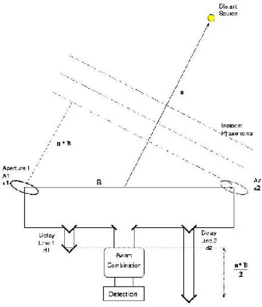
Instrumental Setup Figure2.1depicts the principle of stellar interferometry with two inde- pendent telescopes. Two telescopes, spanning the baseline vectorB, are pointed in directionn towards a source on the sky. Since this source is a great distance away, and therefore considered to be unresolved or “point-like” for the interferometer, the incoming light may be regarded as arriving in plane wavefronts with the wave vector k0 where |k0| = k0 = 2π/λ0 is the wave number1 and λ0 the wavelength. Therefore, n is the negative, normalised wave vector of the incident plane wave, i.e., n=−k0/k0.
The two aperture A1 and A2 each collect a certain section from these wavefronts. The resulting beams are directed by guiding optics towards a beam combination unit where the beams are mixed and therefore interference is produced. This unit may have different configurations depending, for example, on whether the beams are combined in an image plane or in a pupil plane of the telescopes. In an image plane interferometer, the sky is imaged on a detector where the beams are interfered. This will be the case, for example, for the AMBER instrument at the VLTI and the LINC-NIRVANA interferometer on the LBT. In contrast, in a pupil plane interferometer likeMIDI, images of the telescope pupils are overlapped and thus interfered (see Figure 2.2).
Another aspect is the direction in which the interfering beams propagate while they are mixed. Co-axial beams are mixed while propagating in the same direction whereas multi-axial beams propagate in different directions. A pupil plane interferometer with a multi-axial setup shows spatially detectable interferometric fringes, whereas a co-axial setup yields a flat tint. In this case, the interferometric modulation is achieved by a variation of theOptical Path Difference (OPD) between the beams (see below).
MIDI is a co-axial pupil plane interferometer, with the detection taking place in the image plane. All the following considerations are specialised for the MIDI case.
1 Apart from a factor (c/2π), the wave number corresponds to the wave frequencyν0 = c/λ0 (c: speed of light).
Figure 2.1: Principle of stellar interferometry with two independent telescopes. Two telescopes collect light of a source which is directed towards a beam combination unit. TheOptical Path Differencebetween the beams is equalised byDelay Lines. The resulting interference pattern contains information about the observed object. (Drawing adapted fromBoden(2000))
Figure 2.2: Pupil plane beam combiner. The beam combiner plate contains a thin beam splitter layer of symmetric behaviour, i.e., an incident beam is treated the same no matter from which side it occurs.
In this drawing, it is assumed that the layer is sandwiched by two glass plates.
are collected from the same incoming wavefront (see Figure2.1). Losses and phase shifts that are common in both beams are not considered for this purpose. Therefore, it is possible to choose one of the beams as a reference and assign to the other beam allrelativedifferences between the beams, that might be introduced by various effects.
The following effects will be considered explicitly:
An important aspect are atmospheric effects that introduce relative perturbations, which are accounted by a relative atmospheric transfer function
Ta=Ta·eiφa, (2.2)
whereTa is its modulus andφa its phase.
WritingTain this form assumes that the dominant effects of the atmosphere are extinction and the piston effect (see section3.2.3). In particular, relative spatial fluctuations of phase across the aperture pupil do not enter. This assumption is legitimate when the aperture size is clearly smaller than the scale lengthr0 of the atmospheric turbulence, or the phase fluctuations were corrected by spatial filtering or the application of an Adaptive Optics (AO) system.
In each optical train there is a movable mirror which together with some fixed mirrors forms an optical delay line (see Figure 2.1). If the movable mirror is at a distancedaway from its zero position, and one assumes a double-pass optical train, an additional optical path of 2dis introduced. The totalOptical Path Difference (OPD), introduced by purely geometric differences between beam 1 and 2, is then
OP D=n·B+ 2(d1−d2)≡δ. (2.3) The corresponding phase shiftφgeom leads to the complex factor
fgeom=eiφgeom with φgeom=−k0·δ. (2.4)
Instrumental properties that introduce stationary differences between the two beams (e.g., different aperture sizes or bulky optics, like the entrance window, traversed by the beams) can be described by a relative instrumental transfer function
Ti =Ti·eiφi (2.5)
in analogy to the relative atmospheric transfer function.
Now letErbe the reference beam. It follows for the individual contributions in the overlapped beam
Er = Eˆr·exp(iφr),
Et = Eˆt·exp(iφt) = Er·fgeomTaTiTbc
= Eˆr·TaTiTbc·exp[i(φr+φgeom+φa+φi+φbc)] (2.7) and thus for the total interfered beam
E=Er+Et= ˆErexp(iφr)·[1 +TiTaTbc·exp(i(−k0δ+φa+φi+φbc))]. (2.8) The measured signal powerP in this interferometric output is therefore
P =E·E∗ = ˆEr2·[1 +Ti2Ta2Tbc2 + 2TiTaTbc·cos(k0δ−φa−φi−φbc)]. (2.9) Specialisations For simplification, it may be assumed that the atmosphere only introduces disturbances in phase, i.e., Ta = 1. Further, let the design of the two optical paths be ideally matched so thatTi = 1 and Tbc = 1, the latter implying that the beam splitter exactly halves the incident beams. Then, the powerP0 collected by one aperture of areaA from the incoming flux densityF0 =F(λ0) isP0 =AF0 = 2 ˆEr2. With these simplifications, equation (2.9) becomes P =AF0·[1 + cos(k0δ−φa−φbc)] =P0·[1 + cos(k0δ−φa−φbc)], [P] = 1 W. (2.10) For pupil plane interferometers, this last expression can be further evaluated. If the OPDδ is adjusted to zero, then by the symmetry of the interferometer, both interfered output beams should contain equal energy. Changing the OPD will increase the output power of one beam while the other beam will be decreased by the same amount so that the total amount of energy is conserved. This can be explained by the fact that a thin, symmetric beam combiner introduces a phase difference of exactly|φbc|=π/2 between reflected and transmitted beams (Traub,2000) which also accounts for the complementarity of the two beams.
Therefore, it follows withφbc=π/2 for the power contained in one interferometric output P+=AF0·[1 + sin(k0δ−φa)] =P0·[1 + sin(k0δ−φa)] (2.11) and, in analogy, for the complementary output
P− =AF0·[1−sin(k0δ−φa)] =P0·[1−sin(k0δ−φa)]. (2.12) This means that, when changing the OPD, brightness cycles will be observable in the two outputs. Constructive interference will appear in one output and after an OPD step of λ0/2 in the other one. The full modulation corresponds to the total power 2P0 collected by the telescopes.
Likewise, the brightness distribution may vary with position on the sky and wave number so that it should be written asFs(n+∆n, k) ([Fs] = W m−2µm sr−1). Because the projected area collecting light also changes with the offset from the pointing direction, it has to be written A(n+∆n). Another instrument specific may be a response function η(k) that is given by spectral filtering behaviour.
In order to derive equation (2.11), the interferogram of a single unresolved ‘point’ source radiating at wavelengthλ0 was calculated. Having now an extended source, one can consider it as compound of many mutually independent point sources. Furthermore, it can be shown that mixed electric fields of several monochromatic components are incoherent (Born and Wolf,1999, Section 7.5.8). Therefore, one can integrate over all positions of point sources and their spectral range. In general2, equation (2.11) then reads (where the index is dropped):
P(n,B, δ) = Z
dk η(k) Z
∆n
dΩA(n+∆n)Fs(n+∆n, k)·[1 + sin(k·OP D0+φa)] (2.14)
= P0+ Z
dk η(k) Z
∆n
dΩA(n+∆n)Fs(n+∆n, k)·sin(k(∆n·B+δ) +φa).
P0 is the total power collected by one telescope:
P0= Z
dk η(k) Z
∆n
dΩA(n+∆n)Fs(n+∆n, k). (2.15) At this point, one can introduce the correlated flux density Cof the brightness distribution Fs and the aperture functionA as
C(n,B, k) =Ceiψ = Z
∆n
dΩA(n+∆n)Fs(n+∆n, k)e−ik∆n·B, (2.16) where C is the modulus and ψ the complex phase with the phase reference at n. It should be noted that the expression for C, which is the response of the interferometer in a certain config- uration, describes a two-dimensional Fourier transformation of the aperture efficiency weighted brightness distribution on the sky. This could also be expected from the van Cittert-Zernike Theorem in the case of an incoherent source and in small-field approximation, as it is usually present in astronomy.
It is useful to normaliseCby the spectral powerPk received at a certain wave number from the whole source, i.e.,
Pk= Z
∆n
dΩA(n+∆n)Fs(n+∆n, k) , [Pk] = Wµm. (2.17)
2 Note the simplifications leading to equation (2.11).
P(n,B, δ) = P0− Z
dk η(k)={Ce−iφae−ikδ}
= P0+ Z
dk η(k)PkV(n,B, k)·sin(kδ+φa−ψ). (2.19) 2.2.2 Uniform Disk
In order to evaluate equation (2.19) in a more concrete case, one can assume a circular disk source on the sky with angular diameter Θ and spatially uniform brightness distribution Fs. Furthermore,Fs is assumed as constant over the spectral range of the instrument and evaluated at a wave numberk0 which is an effective wave number averaging the spectral behaviour of the intensity distribution of the source (Hanbury Brown et al., 1974, and references therein) (see below). Likewise, Θ should be sufficiently small, so the aperture function may be regarded as constant. Thus, ifρis the angular distance from the centre of the source, the assumptions read Fs(ρ≤Θ/2, k0) =F0 and A(n+∆n) =A0, (2.20) so that the spectral powerPk contained atk0 is
Pk0 =F0·A0·π(Θ/2)2, [Pk0] = Wµm. (2.21) Under these assumptions, it can be shown (Boden,2000) that the correlated flux density for a uniform disk (UD)is
CU D(Θ, B⊥, λ0 = 2π/k0) =CU D·eiψU D =Pk02J1(πΘB⊥/λ0)
πΘB⊥/λ0 ·eiψU D, (2.22) whereB⊥ is the baseline projected in the direction of observation. J1 is the so-called first-order Bessel function of the first kind. The visibility is then given through equation (2.18) by
VU D(Θ, B⊥, λ0) =VU D·eiψU D = 2J1(πΘB⊥/λ0) πΘB⊥/λ0
·eiψU D. (2.23) As the light has to pass through the atmosphere, the interferometer detects in principle CU D ·e−iφa = Pk0VU D ·exp[i(ψU D −φa)], which enters into equation (2.19). Yet, by the turbulent nature of the atmosphere changing the phase φa randomly and thus corrupting the phase information, the phase factor exp[i(ψU D−φa)] is not defined. Therefore, with a two beam stellar interferometer it is usually only possible to access the modulusPk0VU D of the complex visibility. Figure2.3shows the absolute value|VU D|of the modulus of the visibility as a function of its argument (ΘB⊥/λ0) which can be thought of the source diameter Θ in units of (λ0/B⊥).
Inserting these findings in equation (2.19) yields P(n,B, δ) =P0+Pk0
2J1(πΘB⊥/λ0) πΘB⊥/λ0
Z
dk η(k) sin(kδ). (2.24)
3For historic reasons, the absolute value|V|of the modulus V is often sloppily referred by the term “visibility”.
Figure 2.3: Visibility of a Uniform Disk. The absolute value of the modulus of the complex visibility is plotted. The dots indicate visibilities as they would ideally be observed at 10µm with the six baselines provided by the VLTI Unit Telescopes (see section 3.1) on a source with a uniform disk diameter of 22 mas.
2.2.3 Effect of a Finite Bandwidth
In the last step, an example for the effects of a finite spectral bandwidth is presented. Let the overall spectral response η of the instrument be a rectangular bandpass of amplitude η0 = 1 in the range (k0±∆k/2) with|∆k|= 2π∆λ/λ20 and zero elsewhere. The total power collected by one aperture may beP0=Pk0·∆k. Then the integral in equation (2.24) can easily be evaluated, and the power in one interferometric beam, normalised to the total power P0 received by one telescope, becomes
P(n,B, δ) P0
= 1 +
2J1(πΘB⊥/λ0) πΘB⊥/λ0
| {z }
Vobj
·sin(πδ∆λ/λ20) πδ∆λ/λ20
| {z }
Sinst
·sin(2πδ/λ0)
| {z }
Iexp
. (2.25)
The underbraced terms are discussed in the following section.
2.3 Discussion
Basic Oscillation In expression (2.25),Iexp defines the fundamental interference. It is evoked by the experiment when scanning the OPD δ. The frequency is determined by the observing wavelength λ0.
Instrumental Properties Sinst describes the instrument as used for measurements. In gen- eral, Sinst is a product of several factors that describe the state of the instrument like, e.g., unequal aperture size, overlap of the beams, angular alignment, or surface quality of the optics (see sectionA.1). It can be seen as a modulation of the amplitude of the interference and thus as an envelope of the interference. In the present case, a finite wavelength response was considered which results in the given sinc function.
It should be noted that the sinc function contains the coherence length
Lcoh=λ20/∆λ, (2.26)
Figure 2.4:
normalised by the total power received by one aperture, is plotted versus the OPD. Assumptions are an object visibility of 0.75, full transmission in these bands, and a spectral width of 1µm, 3µm and 5µm respectively.
which is the scale length up to which the OPD of the interfering beams must be matched in order to achieve interference. For |δ|=Lcoh the modulation falls to zero. This is seen in Figure 2.4 where some calculated interferogram are plotted as they could be expected for MIDI. They are drawn for λ0 = 10µm, Vobj = 0.75, and for the case that Sinst is only determined by the spectral instrumental properties. One can see how the width of the central wave package varies with spectral width. For comparison, Figure2.5shows an interferogram for a spectral width of roughly 5.5µm like it was recorded during laboratory tests of MIDI. For an OPD larger than Lcoh, i.e.,|δ|> Lcoh, interference is strongly suppressed.
Coherence Length This latter behaviour can be made plausible in the following way (Born and Wolf, 1999, Section 7.5.8). In the interferometer, each single monochromatic component produces a different interference pattern. All these patterns are superposed incoherently, a fact that was actually used to put up equation (2.14) and which in the end yielded the envelope of the total interference pattern. As the OPD increases, the component patterns mutually average each other to a constant level because of their different wavelengths. The coherence length is the typical length of the OPD at which this happens4.
Therefore, in reality when scanning the OPD the visibility of interference fringes decreases with increasing OPD, so that interference is mainly to be expected within the central lobe of the envelope where |δ|< Lcoh.
4In the case of single spectral lines, it is interesting to note that the quantised and statistical nature of light offers an alternative view supposing wave trains of finite length (Born and Wolf,1999, Section 7.5.8). They can only interfere if the OPD is shorter than their roughly common length.
Figure 2.5: Measured broad N band interference pattern. The signal is averaged over four scans and given in arbitrary units. A filter with a spectral width of about 5.5µm was used. (Przygodda,2001)
inst
stars. Their observations deliver an estimation of Sinst so that, in return, Vobj can be derived for the science object which is under investigation.
For a brief outline of the data acquisition process, refer to section2.4.
Object Modeling The full procedure for gaining information about the source is to repeat the measurements and the data reduction process with different baselines. As indicated in Figure2.3, this will yield an according number of visibility points. The proportions between the baselines were chosen in accordance to the ones provided by the Unit Telescopes of the VLTI.
These data can be fitted by applying a model, for example, of a uniform disk to the data points which in turn will yield the source diameter.
In the general case, the source might not be well-described by a uniform disk model be- cause the object brightness becomes fainter towards the edge (limb-darkening effect) or there is effectively no sharply defined edge like, for example, in dust distributions. Retrieving a di- ameter then might be less obvious. Nevertheless, as it was mentioned with equation (2.16), the measured visibility is determined by the Fourier transform of the source brightness distribution.
Therefore, comparing models of astrophysical objects with results from stellar interferometry can help constrain model parameters and improve the understanding of astrophysical processes (see section 5.2).
2.4 A Simple Visibility Measuring Algorithm
As indicated in section 2.3, scanning the OPD is the basic principle of data acquisition in co- axial pupil plane interferometry. This results in an interference signal whose amplitude is the product of an instrumental factorVinst and the object visibility Vobj. If it is assumed thatVinst
can be calibrated, then the full amplitudeM of the interference, which corresponds to the object visibility Vobj, can be restored.
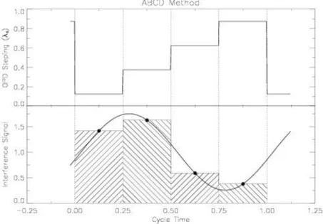
For the MIDI instrument several data acquisition modes are anticipated to retrieve5 the visibility. A quite straightforward mode is called the ABCD method. It is similar to the procedure employed at the Palomar Testbed Interferometer (Colavita, 1999; Colavita et al., 1999). As indicated in Figure2.6, theOPDis adjusted in four steps which are ∆δ =λ0/4 apart.
The associated signals then are (cf. equation (2.11)):
A = M ·sin[(2π/λ0)·δA+φ0] +const., (2.27) B = M ·sin[(2π/λ0)·(δA+ 1·λ0/4) +φ0] +const., (2.28)
5 See also AppendixB.
Figure 2.6: ABCD scan mode. In the bottom diagram, the solid line shows the interferometric signal registered when the OPD were scanned continuously. In the ABCD mode, though, the OPD remains fixed during a quarter of the cycle time as sketched in the top diagram. During this period the interference signal (heavy dots) is integrated which is indicated by the hatched area.
C = M·sin[(2π/λ0)·(δA+ 2·λ0/4) +φ0] +const., (2.29) D = M·sin[(2π/λ0)·(δA+ 3·λ0/4) +φ0] +const., (2.30) where δA is the OPD of the first measured point. φ0 contingently summarises present phase shifts due to instrumental or atmospheric effects. The above set of relations can be rewritten into
A = M·sin[(2π/λ0)·δA+φ0] +const., (2.31) B = M·cos[(2π/λ0)·δA+φ0] +const., (2.32) C = −M ·sin[(2π/λ0)·δA+φ0] +const., (2.33) D = −M ·cos[(2π/λ0)·δA+φ0] +const. (2.34) It follows that for the full modulation (2M) of the signal
2M = q
(A−C)2+ (B−D)2. (2.35)
The phaseφof the first data point with respect to zero OPD is φ= [(2π/λ0)·δA+φ0] = arctan(A−C)
(B−D). (2.36)
Also other combinations of (A, B, C, D) are possible in order to retrieveM and φ. ForM, they may differ in the proportionality factor, which is 2 in equation (2.35).
It is clear that equations (2.27) through (2.30) apply to a single wavelength λ0 at which the fringe contrast is evaluated. For a different wavelengthλ0 the OPD steps do not meet the condition of being one quarter of the wavelength. The four steps of width ∆δ =λ0/4 each will cover more or less than λ0. Therefore, the ABCD method as presented above is only directly
parameters of the VLTI and MIDI.
3.1 The VLTI Environment
3.1.1 Telescopes
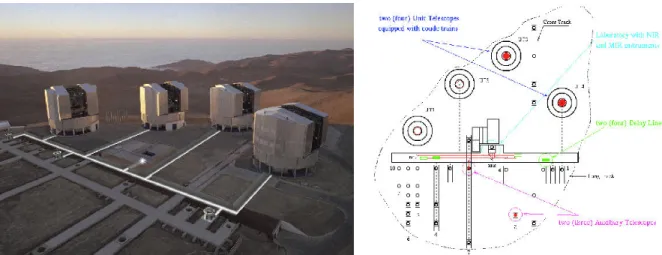
Unit Telescopes (Koehler,1998;Wallander et al.,2000) The main components of the VLTI are fourUnit Telescopes (UT), each with a primary mirror of 8.2 m diameter (8.0 m clear aperture of input pupil). Figure3.1contains an aerial view and a geometric scheme. The VLTI telescopes are specified for operation at wavelengths between roughly 0.5µm and 20µm (Koehler et al., 2002). The angular resolution of a single telescope is defined as
φ= λ
D, (3.1)
which is the angular FWHM of its diffraction limited focal point (Airy disk), where λ is the observation wavelength and D the clear aperture. For a UT, the resolution at λ = 10µm is φU T = 0.2600 (φU T = 0.2100. . .0.3400 forλ= 8. . .13µm). The total of six independent baselines B between two UTs range from 47 m to 130 m. Using two telescopes in interferometric mode, the resolution is again given by equation (3.1) where the baseline1 B enters for the telescope diameter:
φif m= λ
B. (3.2)
Thus, the baseline range translates in interferometric mode at 10µm to a resolution range2 betweenφU Tif m(10µm) = 0.04400 andφU Tif m(10µm) = 0.01600.
Auxiliary Telescopes (Koehler and Flebus, 2000) In addition to the stationary UTs, there will be up to three3 additional Auxiliary Telescopes (AT), with an entrance pupil of 1.8 m and
1 Strictly speaking, it is the baselineprojected into observing direction. Here, zenith observation is assumed.
2 For comparison, the angular diameter of the Sun withD = 0.01 AU as seen from our stellar neighbour α Cen at 1.3 pc distance is 0.00700. The red giant starαOri (Betelgeuse) at 60 pc distance withD= 2.8 au appears under 0.04700.
3 Negotiations are underway to procure a fourthAT.
Table 3.1: Basic parameters of MIDI and the VLTI (selection). Calculated numbers are for 10µm or, where ranges are given, for the N band (8. . . 13µm) respectively.
UTs ATs
Telescope aperture,D 8.0 m 1.8 m
VLTI baselines,B 47. . . 130 m 8. . . 202 m
Telescope Airy diska,b (FWHM) 0.2600 1.100
VLTI spatial resolutiona,b 0.04400. . .0.01600 0.2600. . .0.01000
Field of viewc ≈100 radius
Interferometric field of viewb,c,d ±0.08800. . .0.03200 ±0.5200. . .0.02000
Beam diameter at MIDI input 18 mm
Wavelength range used by MIDI: N band (8. . . 13µm),
expandable to Q band (17. . . 26µm)
Differential dispersion 46µm (1.6. . . 10µm) in 100 m of dry air 0.9µm (10. . . 20µm) Atmospheric stability:
turbulencebtime scale 100 ms, for fringe motion ≤1µmRMS
thermalbtime scale 200 ms, for chopping
Backgroundb,d,e:
from VLTI mirrors 1.5·1011photons/s
from sky 6.2·109photons/s
Signal of N = 0 mag (40 Jy) starb,d,e 2.4·109photons/s 1.2·108photons/s MIDI limiting N magnitude (goal)b,d,e:
without fringe tracking 4 mag (1 Jy) 0.8 mag (20 Jy) external fringe trackingf 9 mag (10 mJy) 5.8 mag (200 mJy) MIDI detector pixel size (50µm)2, 320×240 pixels
full well capacity ≈107 electrons read noise ≈103 electrons per read
a λ/D respectivelyλ/B
bλ= 10µm
csee section3.1.3
d with ∆λ= 5µm (broadband)
ein Airy disk with radiusλ/Dat MIDI detector, see sectionA.1
ffor a broadband on-source integration time of 1000 s
Figure 3.1: View and ground plan of the VLTI. In the aerial view, the white lines indicate the optical path from the Unit Telescopes to the Interferometric Laboratory where the beams are combined. North is up in the layout drawing. (Images: ESO(2002))
thus a resolution of φAT(10µm) = 1.100 (φAT = 0.9200. . .1.500 forλ= 8. . .13µm). Their special property is that they can be relocated to 30 different pre-defined positions with separations of 8 m to 202 m. This yields an interferometric resolution of φATif m(10µm) = 0.2600 down to φATif m(10µm) = 0.01000. The ATs will enable full time use of the VLTI facilities, while UT ob- serving time is shared between single-telescope and interferometric instruments. The smaller diameter of the ATs, reduced by a factor ≈ 4.5 compared to the UTs, means that their light collecting area is (4.5)2 ≈20 times smaller. Considering equation (A.17), their limiting magni- tude will be about 3.2 mag lower. They are therefore likely to be used for bright objects. The current schedule has the ATs becoming operational at Paranal end of 2003.
Siderostats (Derie et al.,2000) Besides the afore-mentioned telescopes, two siderostats (which can be installed at any of the AT locations) are currently available on Paranal. They offer apertures with 0.4 m diameter. Their intention is to provide a facility to test the interferometry subsystems and instruments with little impact on other programmes at the telescopes, but also allow to perform scientific observations on bright objects.
3.1.2 Delay Lines
In order to observe an object interferometrically, it is necessary to direct the beams from the observing telescopes to laboratory instruments that perform coherent superposition. In doing so, the optical paths of the beams must be equalised with a precision of roughly 1/10 of the observing wavelength. In Figure 3.1, the path of the beams through an underground tunnel is shown with white lines. The interferometric laboratory is at the location of the white star.
The geometric OPD between two telescopes depends on the baseline vector B between these telescopes and the observing direction n by (cf. equation (2.3))
OP Dgeom=n·B=B·cosθ, (3.3)
where θ is the angle enclosed by B and n. In Figure 3.2, OP Dgeom is indicated by the line between Telescope 1 and the closest drawn wavefront. For a given object, this value of course changes with sidereal time. The compensation ofOP Dgeom is performed by aDelay Line (DL),
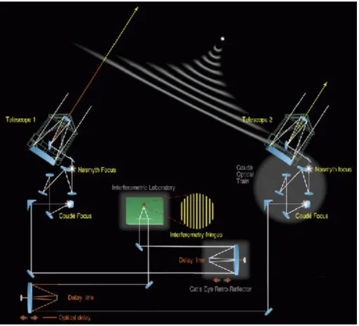
Figure 3.2: VLTI optical train. Beam combination and interference pattern are drawn for an interfer- ometer like AMBER. (Image: ESO(2002))
Figure 3.3: One of the VLTI Delay Lines. Drawing and realisation of the Delay Line cart. (Images:
ESO(2002))
which is shown in Figure 3.3. In principle, the Delay Line is a movable mirror whose position is adjusted so that the OPD of the beams between the entrance pupils and the point of beam combination is nearly canceled. It is realised by a cat’s eye reflector system which can be positioned with an accuracy of only a few dozen nanometers over a stroke length of 60 metres (Derie,2000).
Cancellation of the OPD between two beams by the VLTI Delay Line is specified with an accuracy of ±2.5 mm. Besides the geometric OPD, there is also the additional OP Dadd which is introduced by the atmosphere (see section 3.2.3) and the VLTI optical train. The total internal VLTIfluctuations are estimated to be 0.78µm RMSat 10µm observing wavelength in an exposure time of 290 ms (Koehler et al., 2002). Therefore, an interferometric instrument, requiring zero OPD for measurements, needs an additional Internal Delay Line (IDL) that provides a second step of rapid OPD correction to the precision mentioned before. The IDL for MIDI is discussed in section 4.2. Another possibility is to use a so-called fringe tracker that stabilises the fringe pattern by compensating OP Dadd (see the PRIMA project mentioned in the following section).
3.1.3 Interferometric Instrumentation
After a further reduction of the diameter from 80 mm down to 18 mm and a total of 18 reflec- tions (see Figure 3.2), the beams reach the Interferometric Laboratory where the main VLTI instruments are placed. Figure 3.4shows a floor plan of the lab. At this point, the VLTI offers a Field Of View (FOV), projected back on the sky, of about 100 radius. The full interferometric FOV Θif m around the observing direction is given by the fact that the maximum allowed OPD B·(Θif m/2)additional to the geometric one from equation (3.3) must be shorter than the co- herence length defined by the filter in use of width ∆λand central (effective) wavelengthλc (see equation (2.26)):
B·(Θif m/2)< λ2c
∆λ or (Θif m/2)< λc
B λc
∆λ . (3.4)
B is again the baseline length4 of the stellar interferometer. Observing with a baseline of 100 m at λc = 10µm with ∆λ = 5µm, this yields Θif m ≈ ±0.04000. The wavefront error between two beams as delivered by the VLTI to the instruments is specified with 1.17µmRMS for UT
4 Note remark1on page17.
Figure 3.4: Ground plan of VLTI Interferometric Laboratory. (Image: ESO (2001))
beams and 0.33µmRMSfor AT beams without usage of anAdaptive Optics(see below) system (Koehler et al.,2002).
The following paragraphs shortly describeVLTIsupporting units and the instruments in the Interferometric Laboratory except forMIDI. In section3.3, the design and capabilities of MIDI are focused on.
MACAO (Donaldson et al., 2000) MACAO (Multiple Application Curvature Adaptive Op- tics) is an Adaptive Optics (AO)system which will be installed at several foci of the VLT. The term MACAO-VLTI indicates the application of this AOsystem for use by the VLT interfer- ometer. All four VLT/UT Coud´e foci will be equipped with such a system feeding the VLTI delay lines with a corrected (diffraction limited) IR beam in the range 1.0. . .13.0µm. System performance is expected to show up to 50 % Strehl5 ratio at 2.2µm. The first MACAO-VLTI unit is scheduled for installation on Paranal by end of 2002. The final unit is foreseen to be installed by mid of 2003.
Part ofMACAOis theSystem for Tip-tilt Removal with Avalanche Photodiodes (STRAP).
As outlined in section3.2.3, this unit alone will be able to perform a large part of signal correction forMIDI at 10µm. Instruments at shorter wavelengths, like e.g. AMBER (see below), require the application of the fullMACAO system.
VINCI (Kervella et al.,2000b) The fibre beam combiner VINCI (VLT INterferometer Com- missionning Instrument) works in the K band around 2.2µm. It uses a combination tech- nique proven by the FLUOR (Fiber Linked Unit for Optical Recombination) instrument which has been operational at the IOTA (Infrared-Optical Telescope Array) stellar interferometer on
5 See sectionA.3
referred to as “artificial stars”. These help in aligning the various VLTI instruments, e.g., by providing stable radiation sources. To date, the performance of these light sources is mainly specified at visible and near-infrared wavelengths. For the mid-infrared regime, development is still behind. Experiences gained with MIDI and its laboratory calibration sources (as described in section 4.3) will help constrain requirements and properties.
In the future, it is planned to source out the alignment sub-unit ofVINCIand the calibration sources to a separate VLTIunit called ARAL.
AMBER (Petrov et al.,2000) The science instrument for the near-infrared regime is AMBER (Astronomical Multiple BEam Recombiner). Being designed for eventually interfering three beams in the pupil plane, this instrument will be able to construct images by phase closure techniques. In a first phase, AMBER will operate in the 1. . .2.5µm wavelength range with two UTs. The wavelength coverage will be extended down to 0.6µm at the time the ATs become operational. Due to its working wavelength range, the performance of AMBER will strongly depend on availability of AOsystems. In the K band around 2.2µm, for example, the Fried parameter is r0(2.2µm) = 0.8 m, which is roughly one tenth of the UT aperture size (see section 3.2.3). The magnitude limit of AMBER in the K band is expected to be 20 mag when a bright reference star for AOis available and 14 mag otherwise.
PRIMA (Delplancke et al., 2000) The objective of the planned PRIMA (Phase-Referenced Imaging and Microarcsecond Astrometry) project is to enable simultaneous interferometric ob- servations of two objects that are separated by up to 1 arcmin, without requiring a large contin- uous FOV. The principle of operation relies on finding, within an area of about 1 arcmin around the science target, a sufficiently bright star that can be used as a reference star for the mea- surement and the stabilisation of the science fringe motion induced by atmospheric turbulence, namely the piston effect (see section 3.2.3). This fringe stabilisation will be performed by the FINITO (Fringe-tracking Instrument of NIce and TOrino) respectively an equivalent sub-unit of PRIMA. The performance is expected to yield an OPD fluctuation of less than 0.1µmRMS (Koehler et al., 2002). By allowing longer integration times, this mode increases photometric sensitivity by an expected 3 mag or more. The other interferometric instruments will accordingly benefit from this fringe stabilisation.
Additionally, all optical path lengths of the reference star and of the science star inside the interferometer will be controlled with a laser metrology system, and fluctuations will be compen- sated for by adjusting the Differential Delay Line (DDL) which is also shown in Figure3.4. It will therefore allow to preserve the visibility phase information. This introduces the capability of phase-referenced imaging of science objects with two telescopes and of determining the angular
that highly suppress light from bright stars to detect faint emission from neighbouring dust and possibly massive extra-solar planets. The newly announced Ground-based European Nulling Interferometer Experiment (GENIE) (Gondoin et al., 2002) is a joined ESA/ESO project in order to study technological demands and gain experience in their solution. It could demonstrate the working principle of future space missions like, for example, DARWIN.
3.2 Mid-Infrared Interferometry with MIDI
3.2.1 Scientific motivation
The mid-infrared wavelength range around 10µm is a regime where emission originating from dust plays an important role in astrophysical processes. For matter at temperatures 230. . .370 K, the maximum of blackbody emission lies in the N band. The main scientific topics that will be addressed with MIDI are:
Star formation andYoung Stellar Objects (YSO): size, geometry and structure of proto- stellar cores, circumstellar disks and envelopes; YSO multiplicity, determination of mass ratios
Evolved stars: size, geometry and structure of dust and molecule envelopes aroundAsymp- totic Giant Branch (AGB)stars; spatial pulsation of variable stars; surface structure (e.g., spots)
Substellar objects: aiming at a direct detection and, where possible, spectroscopy of brown dwarfs and hot massive planets by differential interferometric techniques (observationally and technically demanding)
Active Galactic Nuclei (AGN): existence, size, and possibly structure of dust tori
Other programs: e.g., hot stars, the Galactic centre, volcanism in the solar system With the VLTI, it will be possible to extend full interferometric resolution to fainter objects and therefore also to new classes of objects. A detailed description of the scientific prospects of interferometry, not only at 10µm, is found, for example, inParesce(1997).
3.2.2 Technical Aspects
Apart from this scientific motivation for interferometry in the mid-infrared regime, there is another advantage compared to the near-infrared or, to a greater extent, to the visible regime.
Optical and mechanical requirements are less stringent since the demands relax and scale with the wavelength.
On the other side, the mid-infrared regime also suffers from high thermal background pro- duced by the atmosphere, VLTI telescopes, and transfer optics. The signal of a 0 mag object
Figure 3.5: Atmospheric transmission in the N band. Shown for the Mauna Kea observation site on Hawaii (Lord, 1992) at water vapour column of 1.0 mm and air mass AM = 1.5. (With z the zenith angle, the air mass is AM= 1/cosz (L´ena et al.,1998).) Except for a strong absorption around9.5µm due to the ozone layer in the upper atmosphere and a few minor other lines, the atmosphere is highly transparent, in particular between 10µm and 12µm.
is roughly 1 % of the optics background (see section A.1). Therefore, chopping is necessary to extract the source signal from the background. For a typical integration time of 25 ms, which is driven by the need to perform a full measurement within one atmospheric turbulence time scale (see below), the background signal produces about 109 electrons on the detector. Because the detector has a well depth of 107 electrons per pixel, another requirement is to spectrally disperse the signal over at least 100 pixels in order not to saturate or operate in a non-linear regime. Another option is to decrease the integration time and perform repeated short reads of the detector.
3.2.3 Atmospheric Conditions
Ground-based astronomy in the mid-infrared regime is made possible by the atmospheric trans- mission window in the so-called N band between 8µm and 13µm and in the Q band between 17µm and 26µm. The transmission for the N band is shown in Figure 3.5. The atmosphere also affects astronomical observations in respect to the stability of observing conditions. This is discussed in the following paragraphs.
Quantities from Turbulence Theory For a given wavelength λ, the Fried parameter r0
describes the turbulent behaviour of the atmosphere integrated over its total height H. r0 can be interpreted as a scale length, perpendicular to the line of sight, over which the phase of a light wavefront coming from a star may be considered as constant. The atmosphere can be seen as layers of air at a given heighthmoving at a wind speedvw. Turbulence causes density variations and thus fluctuations of the refraction index. The quantity Cn2(h) describes these fluctuations.
Observing at an angle zfrom the zenith, one yields for r0 (Tyson,1998):
r0 ∝λ6/5(cosz)3/5 Z H
0
Cn2(h)dh
!−3/5
. (3.5)
Directly related tor0 is the coherence time,τ0∝r0/vw, which describes the time scale over
Specifics at Paranal Because all these quantities depend on atmospheric properties, they can vary for specific sites, time of day etc. For the VLT(I) on Mt. Paranal, recent values of these quantities can be found in the ESO (1999) reference. Latest measurements appear in Martin et al.(2000). In the year 2000, the median seeing value on Paranal was 0.7500, measured at 0.5µm zenith pointing. This translates to a Fried parameter of r0(0.5µm) = 0.14 m. The median coherence time was 3.6 ms.
By means of equation (3.5), in particular usingr0 ∝λ6/5, it is possible to derive the expected values of the discussed quantities for the N band, namely the Fried parameterrN0 = 5.0 m, the seeing αN = 0.4000, and the coherence time τ0N = 130 ms. These findings imply two main consequences:
1. BecauserN0 is roughly of the aperture size of one Unit Telescope (and, notably, larger than the ATs), the wavefront phase can be considered as almost constant over the aperture.
Therefore, interferometry with the VLTI at 10µm depends little on an Adaptive Optics system, which would correct mainly higher order aberrations in one aperture. Application of a tip-tilt correction provided by a mirror in the Coud´e optical train already compensates signal variations to a high degree (seeMACAO system in section3.1.3).
The main remaining atmospheric effect is the piston difference, i.e., the offset of the wave- front phase, introduced by the atmosphere between the two interfering telescope apertures.
This piston effect, which is a random effect, causes fringe motion, i.e., a shift of the zero OPD position. At 10µm observing wavelength and 290 ms exposure time, it is estimated as 0.63µm RMS for the purely atmospheric contribution, i.e., outside the interferome- ter (Koehler et al., 2002). For a long exposure time, the peak-to-valley value is 30µm (Glindemann,2002).
2. As long as there is no fringe sensor unit installed which compensates for this remaining piston error, all exposures taken by MIDI must be qualitatively shorter thanτ0N, in order to avoid smearing of the interference pattern.
For a quantitative estimation of the maximum possible exposure time,Leinert et al.(1997) chose an approach different to that presented above. A tip-tilt corrected telescope was assumed with a diameter equal to the separation ofUT1 andUT2 at the VLTI, i.e., 54 m.
As a critical condition it was assumed that the corresponding image centroid would move less then 1/10 of the fringe spacing, i.e., 1µm. Considering the bandwidth requirements for such a system, a maximum exposure time of 120 ms was derived. This is essentially the same value derived above.
The equivalence between the two approaches to derive an appropriate exposure time is given in the following argument, again taking into account a frozen atmospheric layer.
As stated above, the phase of a wavefront is considered constant overr0. With the layer moving at a wind speedvw, the phase distribution in the aperture will have changed after
camera MAX at the UKIRT telescope indicates that the typical time scale for these thermal fluctuations is τsky ≈200 ms (Robberto and Herbst,1998). This requires a chopping frequency of 5 Hz in order to calibrate for the sky background.
An expanded treatment of effects of atmospheric turbulence on visibility measurements with MIDI are presented byPorro et al. (2000).
3.3 The MIDI Instrument
MIDI, theMID-infrared Interferometric Instrument, will work in the N band between 8µm and 13µm (Leinert et al.,2000). In a later phase, it is expected to extend MIDI also to the Q band (17. . . 26µm). Figure 3.6 contains a simplified schematic of MIDI. The optical table of MIDI expects two incoming beams of 18 mm diameter which are extracted from the VLTI beams and directed towards the MIDI optics.
3.3.1 Warm Optics
The extracted beams travel through the Warm Optics of MIDI which are mounted on an optical table in front of the instrument housing. Like the VLTI optics, the Warm Optics (and the Cold Optics within the cryostat) are designed such that the same number and kind of reflections occur in each light path. All mirrors involved are gold-coated in order to optimise their reflectivity6 and tilt-adjustable. Both light paths are equipped with a piezoelectric stage carrying a roof mirror7. The piezos have a mechanical stroke of roughly 80µm each and serve as the fast part of the Internal Delay Line and scanned according to operational mode (see section2.4). The piezo stages are further focused on in section4.2. One of the piezo stages is, in addition, mounted on a translation stage with a total mechanical stroke of about 25 mm. This allows static equalisation of the optical path of the beams (see section 3.1.2) to a few wavelengths in the first place so that nominal zero OPD is well within reach of the fast delay line piezo stages.
Another part of the Warm Optics is a set of alignment plates, working at visible light, which are mounted on the Warm Optical Table. They serve as the positional reference for the entire instrument. Together with two alignment telescopes, they are used to adjust the Warm Optics components.
A major group of devices within the Warm Optics is dedicated to the calibration of MIDI.
Directly placed on the Warm Optical Table, there is a black screen which can be heated by about
6 At 10µm, the reflectivity of a gold-coated mirror is usually higher than 99 %.
7 In a roof mirror, two plane mirrors enclose an angle of 90 degrees (see Figure4.1). If it is mounted with the angle opening parallel to the optical table, a beam travelling parallel to the table is exactly reversed (see Figure2.1), independently of the lateral incident direction of the beam.
Figure 3.6: Scheme and overview of MIDI.In front of the dewar lies the Warm Optics bench. In the overview on the far right one can see the extra optical table carrying two of the three calibration light sources.