A Confidence Corridor for Sparse Longitudinal Data Curves

SFB 649 Discussion Paper 2011-002

A Confidence Corridor for Sparse Longitudinal

Data Curves

Shuzhuan Zheng*

Lijian Yang*

Wolfgang Karl Härdle**

*Michigan State University, USA

** Humboldt-Universität zu Berlin, Germany

This research was supported by the Deutsche

Forschungsgemeinschaft through the SFB 649 "Economic Risk".

http://sfb649.wiwi.hu-berlin.de ISSN 1860-5664

SFB 649, Humboldt-Universität zu Berlin Spandauer Straße 1, D-10178 Berlin

S FB

6 4 9

E C O N O M I C

R I S K

B E R L I N

A CONFIDENCE CORRIDOR FOR SPARSE LONGITUDINAL DATA CURVES^∗

By Shuzhuan Zheng¹, Lijian Yang^2,1 and Wolfgang K. H¨ardle^3,4

1Michigan State University,²Soochow University, ³Humboldt-Universit¨at zu Berlin and⁴National Central University

Longitudinal data analysis is a central piece of statistics. The data are curves and they are observed at random locations. This makes the construc- tion of a simultaneous confidence corridor (SCC) (confidence band) for the mean function a challenging task on both the theoretical and the practical side. Here we propose a method based on local linear smoothing that is implemented in the sparse (i.e., low number of nonzero coefficients) mod- elling situation. An SCC is constructed based on recent results obtained in applied probability theory. The precision and performance is demonstrated in a spectrum of simulations and applied to growth curve data. Technically speaking, our paper intensively uses recent insights into extreme value the- ory that are also employed to construct a shoal of confidence intervals (SCI).

1. Introduction. Longitudinal or functional data analysis (FDA) is a central piece of statisti- cal modelling. A well known application is growth curve analysis in biology, medicine and chemistry, see e.g. M¨uller (2009), James, Hastie and Sugar (2000), Ferraty and Vieu (2006) and the references there. Groundbreaking theoretical work on functional data analysis has been done among others by

∗This research was supported by the Deutsche Forschungsgemeinschaft through the CRC 649 “Economic Risk”, NSF Awards DMS 0706518, DMS 1007594, an MSU Dissertation Continuation Fellowship, and a grant from Risk Management Institute, National University of Singapore.

AMS 2000 Classification:Primary 62G08; secondary 62G15 JEL Classification:C14, C33

Keywords and phrases:Longitudinal data, confidence band, Karhunen-Lo`eveL²representation, local linear estimator, extreme value, double sum, strong approximation.

1

Cai and Hall (2006), Cardot, Ferraty and Sarda (2003). Much of this work though is devoted to co- efficient estimation, semiparametric analysis or dimension reduction methods. Research on statistical inference on the mean curve for example is rather scarce although it is potentially important for char- acterization of global properties. To characterize global properties of the unknown function of interest, the simultaneous confidence corridor (SCC) and the shoal of confidence intervals (SCI) are puissant in- struments. They can be applied to test the overall trend or shape of the mean function. Such decisions are critical e.g. in ozone analysis, seeLucas and Diggle (1997)for a longitudinal study on Sitka spruce.

They have pointed out that, in order to assess the cumulative effect of ozone pollution on spruce, an inference on the mean function of spruce growth during the entire experiment rather than at the end of the growth is required. This is one of the many other motivations to develop a new method and its theory to construct an SCC for the mean function of sparse longitudinal data where the measurements are randomly located with random repetitions.

The SCC methodology has been extensively studied in the literature. For the nonparametric regres- sion, seeFan and Zhang (2000)and references there. In this strand of literature though it is not assumed that for family of curves one needs to take care of dependence structures. Wu and Zhao (2007) re- cently constructed a confidence band for the non-stationary mean function, andWang and Yang (2009), Song and Yang (2009)obtained the spline-based analogy for the mean and variance functions. Nonpara- metric time series with specific dependence structures are considered inZhao and Wu (2008). An SCC construction for longitudinal data remains however an open problem.

The major difficulty to construct the SCC for longitudinal data is that the observations within subject are dependent. In this situation, the “Hungarian embedding”, used to construct confidence bands is no longer applicable. The sparse longitudinal data situation has been considered byYao et al. (2005a)for individual trajectories instead of the mean function, while Yao (2007) obtained an SCI for the mean and covariance functions.Ma et al. (2010)constructed the first SCC of the mean function for the sparse longitudinal data through piecewise constant spline. The constructed SCC, however, is nonsmooth and

its convergence rate to the true mean function has suboptimal rate.

Here we propose to construct the SCC for the mean function of the sparse longitudinal data via local linear smoothing. We tackle with this research a variety of interesting issues. First, the proposed SCC allows for the global rather than pointwise inference. Second, the sparse rather than dense longitudinal data setting requires more sophisticated extreme value theory. Third, compared to the piecewise con- stant spline method ofMa et al. (2010), different extreme value results are employed for a local linear estimator that leads to higher accuracy, better coverage, smooth mean curve and smooth SCC, all of which are desirable in the application.

We organize our paper as follows. In Section 2, we state our model and local linear smoothing methodology. In Section 3, we investigate the asymptotic distribution of the maximal deviation of the local linear estimator from the true mean function, which is used to construct the SCC. Section 4 outlines the key procedures to implement the SCC. Section 5 illustrates the performance of the SCC through extensive simulations followed by an empirical example in Section 6 which illustrates the SCC application on growth curve data. Technical proofs are presented in the Appendix.

2. Model and Methodology. Longitudinal data has the form of{X_ij, Y_ij},1≤j≤N_i,1≤i≤ n, in whichXij ∈ X = [a, b] is thej-th random time point for the i-th subject and Yij is the response measured at Xij. For the i-th subject, the sample path is the noisy realization of a continuous time stochastic processξi(x), namely,

Y_ij =ξ_i(X_ij) +σ(X_ij)ε_ij, (2.1) where the errorsεij are i.i.d. withEεij = 0,Eε²_ij = 1, and{ξi(x), x∈ X }are i.i.d. copies of the process {ξ(x), x∈ X }withE∫

Xξ²(x)dx <+∞.

Denote bym(x) =Eξ(x) the regression curve and byG(x, x^′) = Cov{ξ(x), ξ(x^′)} the covariance operator with the Karhunen-Lo`eveL² representation

ξi(x) =m(x) +∑∞

k=1ξikϕk(x), (2.2)

one has the random coefficients {ξ_ik}^∞k=1 uncorrelated with mean 0 and variance 1. Here ϕ_k(x) =

√λkψk(x), where {λk}^∞k=1 and {ψk(x)}^∞k=1 are respectively the eigenvalues and eigenfunctions of G(x, x^′) such that λ1 ≥ λ2 ≥ . . . ≥ 0 and {ψk}^∞_k=1 forms an orthonormal basis of L²(X). There- fore,G(x, x^′) =∑_∞

k=1ϕ_k(x)ϕ_k(x^′) and∫

G(x, x^′)ϕ_k(x^′)dx^′=λ_kϕ_k(x).

In applications, the number of eigenfunctionsψk(x), k= 1,2, ...needs to be chosen by some criterion, seeYao et al. (2005a). In the sparse curve data situation, many practical studies have shown that fitting too many eigenfunctions can heavily degrade the overall fit, see e.g. James, Hastie and Sugar (2000).

Hence, in what follows, we assume thatλ_k= 0 ifk > κ, whereκis a positive constant. Equations (2.1) and (2.2) can then be written as:

Y_ij =m(X_ij) +∑κ

k=1ξ_ikϕ_k(X_ij) +σ(X_ij)ε_ij. (2.3) For convenience, we denote the conditional variance ofYij givenXij=xas

σ²_Y (x) =G(x, x) +σ²(x) =Var(Yij|Xij=x). (2.4) We are interested in the sparse situation where the number of measurementsNi within subject are i.i.d. copies of a positive random integerN1, seeYao et al. (2005a),Yao et al. (2005b),Yao (2007).

To introduce the estimator, denote byK a kernel function,h=h_n >0 a bandwidth andK_h(x) = h⁻¹K(x/h). LetN_T=∑n

i=1N_i be the total sample size and defineY= (Y_ij)_1≤j≤N

i,1≤i≤ntheN_T×1 vector of responses. For any x∈[0,1], letX=X(x) = (1, Xij−x)_1≤j≤N

i,1≤i≤n be the design matrix for linear regression andW=W(x) =N_T⁻¹diag{Kh(X11−x),· · ·, Kh(XnN_n−x)}the kernel weight diagonal matrix. FollowingFan and Gijbels (1996), local linear estimators ofm(x) andm^′(x) are

{mb(x),mc^′(x)}^T= arg min

a,b{Y−X(a, b)^T}^TW{Y−X(a, b)^T}

=(

X^TWX)₋1

X^TWY.

Consequently, withe^T₀= (1,0),mb(x) is written as b

m(x) =e^T₀(

X^TWX)₋1

X^TWY, (2.5)

where the dispersion matrix

X^TWY= diag (1, h)



 s_n,0 s_n,1 sn,1 sn,2



diag (1, h), (2.6)

has for any nonnegative integerl,

s_n,l=s_n,l(x) =N_T⁻¹∑

i,jK_h(X_ij−x){(X_ij−x)/h}^l. (2.7) 3. Main Results. Without loss of generality, assume X = [0,1] and consider the assumptions:

(A1) The mean function m(x)∈C²[0,1], i.e. twice continuously differentiable.

(A2) {Xij}^∞_i=1,j=1^,∞ are i.i.d. with a probability density f(x). The functions f(x), σ(x)and ϕk ∈C¹[0,1]

with f(x)∈[c_f, C_f], σ(x)∈[c_σ, C_σ] and all involved constants are finite and positive.

(A3) The numbers of observations Ni, i = 1,2, . . . are i.i.d. random positive integers with EN₁^r ≤ r!c^r_N, r = 2,3, . . . for some constant cN > 0. (Ni)^∞_i=1,(Xij)^∞_i=1,j=1^,∞ ,(ξik)^∞_i=1,k=1^,κ ,(εij)^∞_i=1,j=1^,∞ are independent, while {ξ_ik}^∞_i=1,k=1^,κ are i.i.d. N (0,1).

(A4) There exists r >5, such that E|ε11|^r<∞.

(A5) The bandwidth h=hn satisfies nh⁴→ ∞, nh⁵logn→0 and h <1/2.

(A6) The kernel function K(x) is a symmetric probability density function supported on [−1,1] and

∈C³[−1,1].

Assumptions (A1), (A2), (A5) and (A6) haven been postulated in many papers related to kernel smoothing. (A3) has been used inYao et al. (2005a). (A4) can be found also inMa et al. (2010).

For a nonnegative integerl and a continuous functionL(x), define:

µ_l,x(L) =













∫1

−x/hv^lL(v)dv, µ_l(L) =∫1

−1v^lL(v)dv,

∫(1−x)/h

−1 v^lL(v)dv,

x∈[0, h) x∈[h,1−h]

x∈(1−h,1]

(3.1)

D_x(L) =µ_2,x(L)µ_0,x(L)−µ²_1,x(L), (3.2)

and the equivalent kernel function, seeFan and Gijbels (1996):

K_x^∗(u) =K(u){µ2,x(K)−µ1,x(K)u}D⁻_x¹(K), K_x,h^∗ (u) =K_x^∗(u/h)/h (3.3) whereD_x⁻¹(K) exists by LemmaA.5. One may verify:

µ0,x(K_x^∗) = 1, µ1,x(K_x^∗) = 0

Dx(K) =µ2(K), K_x^∗(u)≡K(u),∀x∈[h,1−h]. The asymptotic variance function is:

σ²_n(x)^def= ∥K_x^∗∥²2σ_Y² (x) nhf(x)EN1

[ 1 + E(

N₁²−N1

) EN1

G(x, x)f(x)h σ²_Y (x)∥K_x^∗∥²2

+µ1,x

(K_x^∗2) {

σ_Y² (x)f(x)}_′ h

∥K_x^∗∥²2σ_Y² (x)f(x) ]

. (3.4)

Definez_1−α/2^def= Φ⁻¹(1−α/2) and

Q_h(α)^def= a_h+a⁻_h¹[log{√

C(K)/(2π)} −log{−log√

1−α}] (3.5)

witha_h=√

−2 logh,C(K) ={∫1

−1K^′(x)²dx}{∫1

−1K²(x)dx}⁻¹. THEOREM 3.1. Under Assumptions (A1)-(A6), for any α∈(0,1)

nlim→∞P{sup_x∈[0,1]|mb(x)−m(x)|/σ_n(x)≤Q_h(α)}= 1−α,

nlim→∞P{|mb(x)−m(x)|/σ_n(x)≤z_1−α/2}= 1−α,∀x∈[0,1], withσ²_n(x)andQh(α)given in (3.4) and (3.5).

By Theorem3.1, we construct the SCC and SCI form(x) as follows,

COROLLARY 3.1. Assume (A1)-(A6). A100 (1−α) %simultaneous confidence corridor (SCC) form(x)is:

[mb(x)±σ_n(x)Q_h(α)]. (3.6)

A shoal of confidence intervals (SCI) is given by:

[mb(x)±σn(x)z_1−α/2]

. (3.7)

A simple approximation ofσ²_n(x) is given by:

σ²_n,IID(x) = ∥K_x^∗∥²₂σ_Y² (x) nhf(x)EN1

. (3.8)

PROPOSITION 3.1. Given (A2), (A3) and (A6), thensup_x∈[0,1]σ⁻_n¹(x)σn,IID(x)−1=O(h). Usingσ²_n,IID(x) instead ofσ²_n(x) is equivalent to treat{Xij, Yij},1≤j≤Ni,1≤i≤nas i.i.d data, which implies that the longitudinal dependence structure is negligible in case of sparsity. This was also observed byMa et al. (2010),Wang et al. (2005).

4. Implementation. Now we outline the construction of the SCC and SCI. Recall the definition of mb (x). The practical implementation of (3.6) and (3.7) is via estimating EN1, f(x) and σY (x), see Wang and Yang (2009) and references therein. The quantity EN₁ is estimated by N_T/n and the estimator of the densityf(x) is

fb(x) =N_T⁻¹∑n i=1

∑Ni

j=1Kh(Xij−x). (4.1)

The local linear estimatorbσY (x) =ba1 results from:

(ba₁,bb₁ )

= arg min

a₁,b₁

∑n i=1

∑N_i j=1

{bε²_ij−a₁−b₁(X_ij−x)}2

w_ij,

where εb_ij = Y_ij −mb(X_ij), w_ij = N_T⁻¹K_h(X_ij−x) and h = N_T^−1/5(logn)⁻¹ satisfying (A5). The consistency offb(x) andσbY (x) is proved e.g. inLi and Hsing (2010),Yao et al. (2005a). Therefore, the SCCmb(x)±σˆn,IID(x)Qh(α) and the SCI mb(x)±ˆσn,IID(x)z_1−α/2 both have asymptotic confidence level 1−α.

5. Monte Carlo Studies. This section checks the finite sample performance of the SCC. The data are generated from (2.1) withκ= 2:

Yij =m(Xij) +∑2

k=1ξikϕk(Xij) +σ(Xij)εij,

withm(x) = sin{2π(x−1/2)},ϕ1(x) =−0.2 cos{π(x−1/2)},ϕ2(x) = 0.1 sin{π(x−1/2)},σ(x) = exp{3(x−0.5)²}/[1 + exp{3(x−0.5)²}] andX ∼U [0,1], ξ_k ∼N (0,1), ε_ij ∼N (0,1), whileN_i has a

discrete uniform distribution from 5, . . . ,15 and nvaries: 20,50,100,200. The confidence level is set to:

1−α= 0.95,0.99.

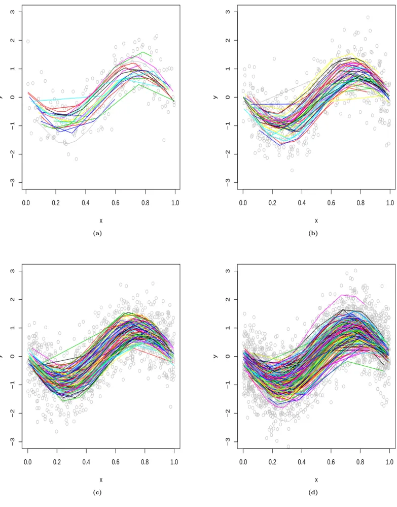
(Insert Figure1“Dataplot and trajectories” about here)

Table 1

Empirical coverage from 200 replications n 1−α= 0.95 1−α= 0.99

20 0.925 0.965

50 0.940 0.980

100 0.950 0.995

200 0.955 0.990

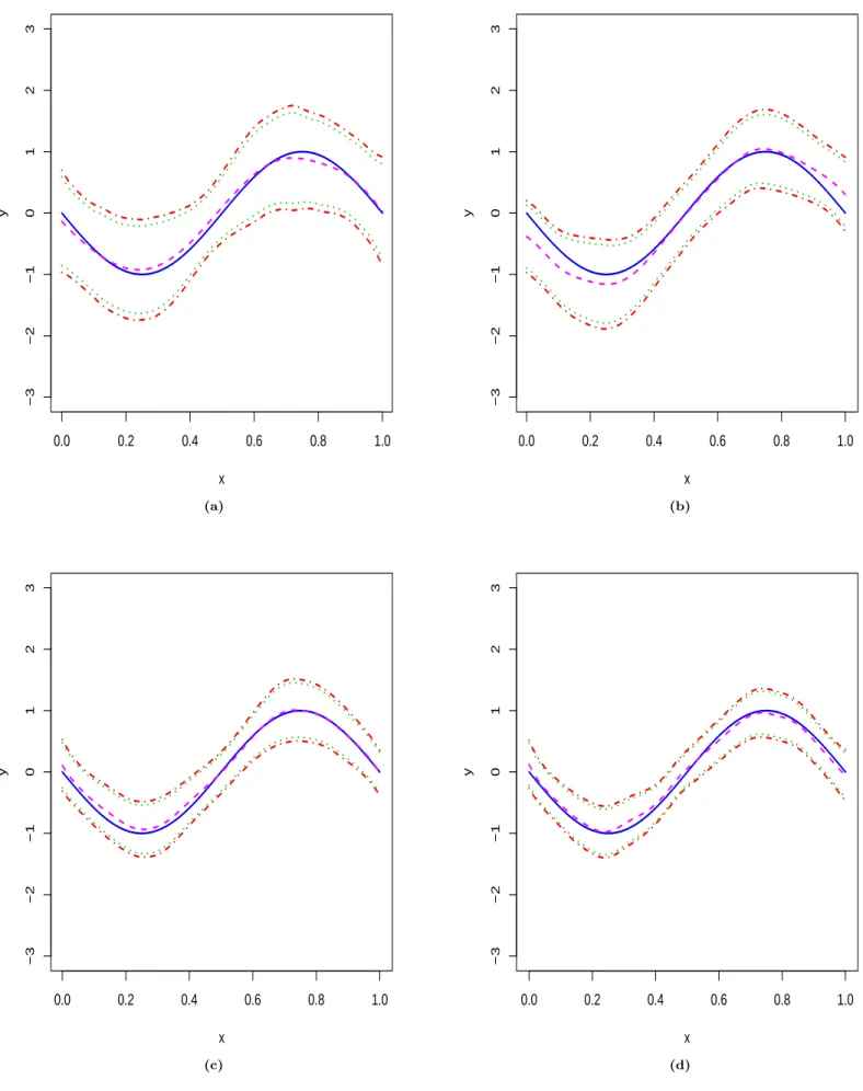
The empirical coverage is reported in Table1. The data are displayed in Figure1. Clearly, the coverage approaches the nominal confidence levels asnincreases, see Theorem3.1. Coverage frequencies remain stable if the bandwidths’ slightly vary. In practice, one can choose bandwidths adaptively to achieve better performance. The theoretical study of this issue would require too much space here. We therefore do not pursue this. Figure2plots the SCCs with 95% and 99% confidence levels. The above studies have illustrated the reliability of our method, which actually ensures the application of the SCC including the true curve for the real data in Section 6.

(Insert Figure2“The 95% and 99% SCCs of the mean curve” about here)

6. Application. Now we apply the SCC and SCI to a longitudinal study of growth curve data. The data curve analysis is a key in the studies of human skeletal health. These data consist of measurements Y_ij, spinal bone mineral density (g/cm²), forn= 286 people. However,N_i, the number of measurements for each individual, is between 2 and 4 (sparsity), andXij, the time points of measurements (aged 8.8–

26.2 yr), varies among individuals.

An earlier study of the growth curve data inJames, Hastie and Sugar (2000)developed the pointwise inference of the mean function. Using the bootstrap method, they constructed the confidence intervals to test the mean curve at points of interest, e.g. the fastest growth point at about 15 yr. In our study, this task can be also done via constructing the SCI by (3.7). However, its computation is much faster than the bootstrap procedures. Furthermore, we will use the SCC to examine the global shape of the mean

curve on the whole domain, such as the upward or downward trend at different stages, the acceleration or plateau during different periods.

(Insert Figure3“Growth curve data and the SCCs & SCIs of its mean curve” about here) Figure3(a) exhibits the scatter plot of the spinal bone density v.s. the age. Figure3(b), (c) and (d) depict the SCCs and SCIs of the population mean of the growth curve data, at the confidence levels of 90%, 95% and 99%, respectively. For the pointwise inference, James, Hastie and Sugar (2000) and our method share similar SCIs. However, testing the global shape of the growth curve, the constructed SCCs can indicate that the spinal bone density at mean level increases with age, but the bone growth is accelerated during early adolescence (9-15 yr) whereas it reaches the plateau during late puberty (16-26 yr). An R algorithm of our method has been provided on www.quantlet.org.

APPENDIX .

A.1. Preliminaries. We introduce Lemmas (A.1)-(A.4) for the proof of Theorem3.1(Appendix A.2). For the details of LemmaA.1, seeCierco-Ayrolles et al (2003),Zheng, Yang and H¨ardle (2010).

LEMMA A.1. [Cierco-Ayrolles, Croquette and Delmas (2003)] Let X(t) be a Gaussian process with almost surelyC¹ sample paths on[0, T]. Then

P{|X(0)|> u}+E[(

U_u^X[0, T] +D^X_−u[0, T])

I_{|X(0)|6u}]

(A.1)

−1 2E(

U_u^X[0, T] +D₋^X_u[0, T])[2]

≤P{sup_x∈[0,T]|X(t)|> u} ≤ P{|X(0)|> u}+E[(

U_u^X[0, T] +D₋^X_u[0, T])

I_{|X(0)|6u}] .

LEMMA A.2. [Theorem 1 of Cierco-Ayrolles, Croquette and Delmas (2003)] Suppose X is a C¹ real-valued Gaussian process defined on an intervalIand{X(t), X(s), X^′(t), X^′(s)}is non-degenerate

∀t̸=s,(t, s)∈I². Then, denoting pV the probability density of a random vectorV: E(U_u^X[I]^[2]) =

∫

I²

∫

(0,∞)²

|x^′₁| |x^′₂|pX_t;X_s;X_t^′;Xs′(u;u;x^′₁;x^′₂)dx^′₁dx^′₂dtds,

E(

U_u^X[I]D^X_−u[I])

=

∫

I²

∫ +∞ 0

∫ 0

−∞|x^′₁| |x^′₂|p_Xt;Xs;X′

t;X_s^′(u;−u;x^′₁;x^′₂)dx^′₁dx^′₂dtds.

LEMMA A.3. [Theorem 2.6.7 of Cs˝org˝o and R´ev´esz (1981)] Suppose that ξ_i,1 ≤i≤n are i.i.d.

withEξ1= 0,Eξ²₁= 1andH(x)>0 (x≥0)is an increasing continuous function such thatx^−2−γH(x) is increasing for some γ > 0 and x⁻¹logH(x) is decreasing with EH(|ξ1|) < ∞. Then there exist constantsC₁, C₂, a >0which depend only on the distribution ofξ₁and a sequence of Brownian motions {Wn(t),0≤t <∞}^∞n=1 such that for any {xn}^∞n=1 satisfying H⁻¹(n) < xn < C1(nlogn)^1/2 and Sk=∑k

i=1ξi

P{max1≤k≤n|Sk−Wn(k)|> xn} ≤C2n{H(axn)}⁻¹.

LEMMA A.4. [Theorem 1.2 of Bosq (1996)]Suppose that ξi,1 ≤ i ≤ n are i.i.d. with σ² = Eξ²₁,Eξ1 = 0 and there exists c > 0 such that for r = 3,4, ...,E|ξ1|^r ≤ c^r−2r!Eξ²₁ < +∞, then for eachn >1,t >0,P (|S_n| ≥√

nσt)≤2 exp{−t²(4 + 2ct/√

nσ)⁻¹}.

A.2. Proof of Theorem 3.1. Throughout this section, for functionsan(x) and bn(x),an(x) =

U{b_n(x)} anda_n(x) =U {b_n(x)}respectively means that, as n→ ∞, sup_x∈[0,1]|a_n(x)/b_n(x)|=_O(1) and sup_x∈[0,1]|an(x)/bn(x)| = O(1). In addition, an(x) = Ua.s.{bn(x)} and an(x) = Ua.s.{bn(x)} respectively means that, asn→ ∞,an(x) =U{bn(x)}andan(x) =U {bn(x)}almost surely, andOa.s.,

Op,Oa.s.,Op are similarly defined.

We denotem= (m(X_ij)),ε= (σ(X_ij)ε_ij),ξ_k= (ξ_ikφ_k(X_ij)). The signal and noise decomposition X^TWY=X^TWm+∑κ

k=1X^TWξ_k+X^TWεimplies that, b

m(x)−m(x) =me(x)−m(x) +ee(x), (A.2) e

e(x) =∑κ k=1

ξek(x) +ε(x),e whereξek(x) =e^T₀(X^TWX)⁻¹X^TWξ_k andeε(x) =e^T₀(X^TWX)⁻¹X^TWε.

The error structure in (A.2) allows one to investigate the asymptotics of sup_x∈[0,1]|ee(x)/σn(x)|and sup_x∈[0,1]|{me(x)−m(x)}/σ_n(x)|separately in LemmasA.6-A.14, with σ_n(x) given in (3.4).

We introduce some more notations, defining

Dx=



 µ_2,x(K) −µ_1,x(K)

−µ1,x(K) µ0,x(K)



, (A.3)

withµl,x(K) given in (3.1) b

ε(x) =f⁻¹(x)N_T⁻¹∑

i,jK_x,h^∗ (X_ij−x)σ(X_ij)ε_ij, (A.4) ξb_k(x) =f⁻¹(x)N_T⁻¹∑

i,jK_x,h^∗ (X_ij−x)ϕ_k(X_ij)ξ_ik, (A.5) withK_x,h^∗ (u) given in (3.3)

Rij,ε(x) =K_x,h^∗ (Xij−x)Dx(K)σ(Xij), (A.6) Rik,ξ_k =∑N_i

j=1K_x,h^∗ (Xij−x)Dx(K)ϕk(Xij), (A.7) withD_x(K) given in (3.2)

σ_ε,n² (x) =f⁻²(x)N_T⁻²D⁻_x²(K)∑

i,jR²_ij,ε(x), (A.8)

σ_ξ²_k,n(x) =f⁻²(x)N_T⁻²D⁻_x²(K)∑n

i=1R²_ik,ξk(x), (A.9) Cx(K) =µ_0,x{K_x^∗′(x)²}

µ_0,x{K_x^∗(x)²} −µ²_0,x{K_x^∗(x)K_x^∗′(x)}

µ²_0,x{K_x^∗(x)²} , (A.10) where K_x^∗′(x) = dK_x^∗(x)/dx, µl,x(L) given in (3.1). It is easily verified that Cx(K) = C(K), ∀x∈ [h,1−h] withC(K) given in (3.5).

LEMMA A.5. Under Assumptions (A5)-(A6), forx∈[0,1]

0< D0(K)≤Dx(K)≤D1/2(K) =µ2(K)<+∞, (A.11) whilesup_x∈[0,1]|Cx(K)|<∞.

Proof.See Appendix B,Zheng, Yang and H¨ardle (2010).

LEMMA A.6. Under Assumptions (A1)-(A6), forD_x(K)given in (3.2) andD_x in (A.3), (X^TWX)−1

=f⁻¹(x) diag(

1, h⁻¹) {

D⁻_x¹(K)Dx+ ∆1,n(x)} diag(

1, h⁻¹) asn→ ∞, where the2×2 random matrices∆1,n(x) =U(h) +Ua.s.{√

logn/(nh)}.

Proof.For notational simplicity, letx∈[h,1−h], we investigate sn,l(x), l= 0,1,2, given in (2.7).

|s_n,0(x)−f(x)| ≤n(EN₁)N_T⁻¹−1

(nEN₁)⁻¹∑n i=1

∑N_i

j=1K_h(X_ij−x)

+ (A.12)

|EKh(Xij−x)−f(x)|+

(nEN1)⁻¹∑n i=1

∑N_i

j=1Kh(Xij−x)−EKh(Xij−x)

=I1(x) +I2(x) +I3(x). Clearly,I2(x) =U(

h²)

andE{Kh(Xij−x)}^r=U( h^1−r)

forr≥2. DefineI3(x) = (nEN1)⁻¹|∑n i=1ζi,h| withζ_i,h=∑N_i

j=1K_h(X_ij−x)−EK_h(X_ij−x)EN₁. For largen, E|ζi,h|^r=E

∑Ni

j=1Kh(Xij−x)−EKh(Xij−x)EN1

^r≤ (A.13)

2^r−1[E{∑N_i

j=1K_h(X_ij−x)}^r+{EK_h(X_ij−x)EN₁}^r]≤ 2^rE{∑N_i

j=1Kh(Xij−x)}^r= 2^rE





r1+...+r∑_Ni=r 0≤r₁,...,r_Ni≤r

( r r₁...r_Ni

)∏N_i i=1

E{Kh(Xij−x)}^ri





≤2^rE [

N_i^{r r1+...+r}max^Ni=r

0≤r₁,..., r_Ni≤r N_i

∏

i=1

E{Kh(Xij−x)}^ri ]

≤2^r(EN₁^r)Crh^1−r≤Cζr!h^1−r.

It can be next verified that E(ζi,h)² = (EN1)h⁻¹f(x)∫

K²(v)dv{1 +U(1)}. Hence, ∃ C_ζ^′ > c^′_ζ > 0 such that c^′_ζh⁻¹ < E(ζi,h)² < C_ζ^′h⁻¹ , i.e., E|ζi,h|^r ≤ c^r_∗⁻²r!E(ζi,h)² with c_∗ = (Cζ/c^′_ζ)^r−21 h⁻¹, see (A.13). In fact, it implies {ζi,h}ⁿ_i=1 satisfies Cram´er’s Condition. Therefore, applying Lemma A.4 to

∑n

i=1ζ_i,h, for largenand largeδ >0, one shows P{I3(x)> δ√

logn/(nh)} ≤ 2 exp[−(EN₁)²δ²logn{4C_ζ^′ + 2δEN₁(

C_ζ/c^′_ζ)1/(r−2)√

logn/(nh)}⁻¹]≤2n^−Cδ2≤2n⁻⁸.

Now discretizeh=x₀< x₁<· · ·< x_Mn= 1−hwithM_n=n⁴and then, P{max^M_j=0ⁿ I3(xj)> δ√

logn/(nh)} ≤∑M_n

j=0P{|I3(x)|> δ√

logn/(nh)} ≤2n⁻⁴, and hence the Borel-Contelli Lemma implies that max^M_j=0ⁿI₃(x_j) =Oa.s.{√

logn/(nh)}. It is also clear that,

sup_{x∈[h,1−h]}I3(x)≤max^M_j=0ⁿI3(xj) + max^M_j=0ⁿ⁻¹sup_{x∈[xj,xj+1]}|I3(xj)−I3(x)|

≤ Oa.s.{√

logn/(nh)}+U{

(1−2h)/( nh⁴)}

=Oa.s.{√

logn/(nh)}, which by the definition ofI3(x) implies that

(nEN1)⁻¹∑n i=1

∑Ni

j=1Kh(Xij−x) =EKh(Xij−x) +Ua.s.{√

logn/(nh)} (A.14)

=f(x) +U(h²) +Ua.s.{√

logn/(nh)}. Applying LemmaA.4forNT, one has|(nEN1)/NT−1|=Oa.s{√

logn/n}and (A.14) also implies that sup

x∈[h,1−h]

I1(x) =Oa.s.(√

logn/n). Now, by (A.12),sn,0(x) =f(x) +U( h²)

+Ua.s.{√

logn/(nh)}. Similarly,sn,1(x) =U(h) +Ua.s.{√

logn/(nh)}andsn,2(x) =f(x)µ2(K) +U(h) +Ua.s.{√

logn/(nh)} which imply thatX^TWXcan be written as

f(x) diag(1, h)[diag{1, µ2(K)}+U(h) +Ua.s.{√

logn/(nh)}] diag(1, h).

Finally, the inverse of this matrix is concluded as this lemma.

LEMMA A.7. Under Assumptions (A1)-(A6), asn→ ∞,∥me(x)−m(x)∥_∞=Oa.s.

(h²) .

Proof.See Proof of Theorem 6.5, page 268 ofFan and Yao (2005).

LEMMA A.8. Under Assumptions (A1)-(A6), forbε(x) andξbk(x) given in (A.4) and (A.5), e

e(x) ={1 + ∆2,n(x)} {bε(x) +∑κ k=1

ξbk(x)}

asn→ ∞, where the2×2 random matrices∆_2,n(x) =U(h) +Ua.s.{√

logn/(nh)}.

Proof. For notational simplicity, let x ∈ [h,1−h], therefore bε(x) +∑κ

k=1ξb_k(x) = f⁻¹(x)T₀(x) withTl, l= 0,1 defined as

Tl(x) =N_T⁻¹∑

i,jKh(Xij−x){(Xij−x)/h}^l{σ(Xij)εij+∑κ

k=1ϕk(Xij)ξik}. LemmaA.6shows that for ∆_1,n(x) given in LemmaA.6

e

e(x) =f⁻¹(x)e^T₀diag(

1, h⁻¹) [ diag{

1, µ⁻₂¹(K)}

+ ∆_1,n(x)]

{T₀(x), T₁(x)}^T,

i.e.,ee(x) ={1 + ∆1,n(x)}f⁻¹(x)T0(x). Therefore, this lemma holds.

LetXij,1≤i≤n,1≤j≤Ni be descendingly ordered asX_(t), 1≤t≤NT, Sq =∑q

t=1ε_(t) where ε_(t)is corresponding in index toX_(t).

LEMMA A.9. Given (A1)-(A6), then there exists a sequence of Wiener processes {W_NT(t)}^N_t=1^T independent of {Ni, Xij, ξi 1 ≤ i ≤n, 1 ≤j ≤ Ni, 1 ≤ k ≤κ} such that as n → ∞ and for some t^′ >2/5

∥bε(x)−εbN_T(x)∥_∞=Oa.s.(n^−t′), withεb_NT(x) ={N_Tf(x)}⁻¹∑N_T

t=1K_x,h^∗ (

X_(t)−x) σ(

X_(t))

{W_NT(t)−W_NT(t−1)}.

Proof.Without loss of generality, let x∈ [h,1−h]. By Lemma A.3, let H(x) = x^r, r > 5 (As- sumption A4) andxn =n^s, s∈(

2r⁻¹,2/5)

. It is easy to verify that{ ε_(t)}N_T

t=1satisfies the conditions of LemmaA.3andnH⁻¹(axn) =a^−rn^1−rs=O(n^−s′) for somes^′>1. Therefore, there exists a sequence of Wiener process {W_NT(t)}^Nt=1^T independent of {N_i, X_ij, ξ_i 1 ≤ i ≤ n, 1 ≤ j ≤ N_i, 1 ≤ k ≤ κ} such thatP{MN_T> n^s} ≤C2n^−s′ with MN_T = max1≤q≤N_T|Sq−WN_T(q)| and hence Borel-Cantelli Lemma warrants thatMN_T =Oa.s(n^s).

The technique of summation by parts implies that sup

x∈[h,1−h]

|bε(x)−εbN_T(x)| ≤ sup

x∈[h,1−h]

N_T⁻¹c⁻_f¹|Kh

(X(N_T)−x) σ(

X(N_T)

){WN_T(NT)−SN_T} (A.15)

+∑NT−1 t=1 {Kh

(X(t)−x) σ(

X(t)

)−Kh

(X(t+1)−x) σ(

X(t+1)

)} ≤h⁻¹MNTN_T⁻¹c⁻_f¹×

sup

x∈[h,1−h]

[ 3C_KC_σ+∑X_(t)∈[x−h,x+h]

1≤t≤N_T−1 |K{(

X_(t)−x) /h}σ(

X_(t))

−K{(

X_(t+1)−x) /h}σ(

X_(t+1))

|].

Since|ab−cd| ≤ |a||b−d|+|b||a−c|+|a−c||b−d|, (A.15) is bounded by h⁻¹MN_TN_T⁻¹c⁻_f¹ sup

x∈[h,1−h]

[ 3CKCσ+∑X_(t)∈[x−h,x+h]

1≤t≤NT−1 2CK×

|σ( X_(t))

−σ( X_(t+1))

|+Cσ|K{(

X_(t)−x)

/h} −K{(

X_(t+1)−x) /h}|].

Therefore,∃constantsL¹_K,σ, L²_K,σ, C andC^′ such that (A.15) is bounded by h⁻¹M_NTN_T⁻¹c⁻_f¹ sup

x∈[h,1−h]

( 3C_KC_σ+L¹_K,σ∑X_(t)∈[x−h,x+h]

1≤t≤N_T−1 |X_(t)−X_(t+1)|+ L²_K,σh⁻¹∑X_(t)∈[x−h,x+h]

1≤t≤N_T−1 |X_(t)−X_(t+1)|)≤h⁻¹MN_TN_T⁻¹(C+C^′h). Namely sup_{x∈[h,1−h]}|bε(x)−bε_NT(x)|=Oa.s(h⁻¹n^s−1) and by assumption (A5), one obtains

sup

x∈[h,1−h]

|bεNT(x)−εb(x)|=Oa.s.(n^−t

′

), t^′ >2/5.

This completes the proof.

LEMMA A.10. Under Assumptions (A1)-(A6), asn→ ∞, N_T⁻¹∑

i,jR²_ij,ε(x)−ER²_11,ε(x)

∞=Oa.s.{√

logn/(nh)}, N_T⁻¹∑n

i=1

∑κ k=1R²_ik,ξ

k(x)−(EN₁)⁻¹∑κ

k=1ER²_1k,ξ

k(x)

∞=Oa.s.{√

logn/(nh)}, withRij,ε(x)andRik,ξ_k(x)given in (A.6) and (A.7).