A Dynamic Day-ahead Paratransit Planning Problem
Maria L.A.G. Cremers
∗Willem K. Klein Haneveld Maarten H. van der Vlerk
Department of Operations University of Groningen P.O. Box 800, 9700 AV Groningen
the Netherlands October 4, 2007
Abstract
We consider a dynamic planning problem for the transport of elderly and disabled people. The focus is on a decision to make one day ahead:
which requests to serve with own vehicles, and which ones to assign to subcontractors, under uncertainty of late requests which are gradually re- vealed during the day of operation. We call this problem the Dynamic Day-ahead Paratransit Planning problem. The developed model is a non- standard two-stage recourse model in which ideas from stochastic pro- gramming and online optimization are combined: in the first stage clus- tered requests are assigned to vehicles, and in the dynamic second-stage problem an event-driven approach is used to cluster the late requests once they are revealed and subsequently assign them to vehicles. A genetic al- gorithm is used to solve the model. Computational results are presented for randomly generated data sets. Furthermore, a comparison is made to a similar problem we studied earlier in which the simplifying but unreal- istic assumption has been made that all late requests are revealed at the beginning of the day of operation.
Keywords: Paratransit Transport, Stochastic Programming, Online Op- timization
∗Email: m.l.a.g.cremers@rug.nl
1 Introduction
We consider a dynamic planning problem for the door-to-door transport of el- derly and disabled people. In particular, since already one day before the day of operation (day-ahead) it is known that there are not enough own vehicles to serve all requests, we focus on a decision to make day-ahead: which requests to assign to subcontractors, and which requests to serve with own vehicles? We will call this problem the Dynamic Day-ahead Paratransit Planning (DDaPP) problem. A typical aspect of the DDaPP problem is that only part of the re- quests are known day-ahead and more requests become known on the day of operation itself. We will focus on this uncertainty with respect to late requests, and on the clustering of requests into routes. Clustering ensures that less ve- hicles are needed to serve all requests. The decision criterion of the DDaPP problem is the expected costs of serving all requests, which depends to a large extent on the degree of clustering.
In the literature, several studies can be found on the door-to-door trans- portation problem for elderly and disabled people (e.g. [2, 4, 5, 6, 13, 15, 18]).
In this problem, a set of service requests is given, as well as a vehicle fleet. Each request consists of the number of customers, a pickup location (origin) and de- livery location (destination), and a desired time for pickup or delivery. The aim is to find a set of minimum cost vehicle routes subject to constraints regarding, among others, vehicle capacity and service measures.
A typical aspect of the door-to-door transportation problem for elderly and disabled people (paratransit problem) is that there are various types of cus- tomers, mostly depending on physical characteristics (e.g., ambulatory cus- tomers, those in folding or non-folding wheelchairs, and those needing special assistance). To accommodate for the various types of customers, the vehicle fleet is often heterogeneous. Each vehicle type has its own capacity depending on the customer type. In addition to the own vehicle fleet, sometimes taxis are used, mainly to transport ambulatory customers during peak hours.
Service measures are important in the paratransit problem and can include waiting time, excess ride time due to detours made because of combined re- quests, and deviations from the desired pickup or delivery time. These measures can either be included in the (multi-criteria) objective function or added to the set of constraints. In the latter case, a bound for each measure needs to be prescribed.
In practice, only part of the requests are known before the start of the day of operation; the remaining requests are gradually revealed during that day.
This dynamic version of the problem is much harder to solve than the static version, in which all requests are assumed to be known beforehand. Of all studies mentioned above, only the studies of Madsen et al. [15] and Attanasio et al. [2]
consider the dynamic version. Various options exist to handle the uncertainty with respect to the late requests. Both Madsen et al. [15] and Attanasio et al.
[2] construct (optimal) vehicle routes for the known requests, and then use an insertion heuristic to include new requests.
As opposed to all other studies, which look at the paratransit problem on
the day of operation (tomorrow), we consider the paratransit problem one day before the day of operation (today). At this time, many requests are already known which makes it possible to assign already today some of the early requests to subcontractors. Since there are not enough own vehicles to serve all requests, and for day-ahead subcontracting better rates have been agreed upon than for subcontracting on the day of operation, it can be profitable to do so. Another advantage of considering the paratransit problem day-ahead, which is very im- portant in practice, is that tomorrow the set of requests requiring scheduling is smaller so that a solution can be found faster. Moreover, some simplifying assumptions can be made which diminish the complexity of the problem and resulting model. For example, the vehicle routes do not need to be determined in detail in our problem.
In a previous paper [7], we studied the (semi-dynamic) day-ahead paratran- sit planning problem. This problem is very similar to the DDaPP problem, except that we have made there the unrealistic but simplifying assumption that all late requests become known early tomorrow morning, as opposed to the DDaPP problem at hand in which we assume the late requests to be gradually revealed during that day. In [7], we developed a two-stage recourse model in which the first stage models today. Only the early requests are handled explic- itly and probabilistic information is used on the late requests. The second-stage problem is a static problem, modeling tomorrow, in which all late requests are known at the outset. For the DDaPP problem, we have also developed a two- stage recourse model. The first stage is equal to the first stage of the simplified problem, but now the second-stage problem, again modeling tomorrow, is ady- namicproblem in which late requests are gradually revealed and immediate or online decisions are required. Thus, the second stage is an online optimization problem. In this problem, no information is assumed to be known about future requests and their time of arrival. Hence, like in traditional recourse problems from stochastic programming, we model the uncertainty about tomorrow’s re- quests by assuming probabilistic information (scenarios), allowing to calculate the expected future costs of each current (first-stage) decision. However, unlike the stochastic programming paradigm, in the second stage we do not allow to use (probabilistic) information about the remaining future. (See Section 3 for a short discussion of multi-stage recourse models). Essentially, as soon as a new request arrives, a decision needs to be made, without any information on possible further requests. In this sense, our second-stage problem is an online optimization problem. In online optimization, not only the assumption to have probabilistic information as represented by scenarios is non-standard, but also the two-stage approach itself. As far as we know, no such combination of ideas from stochastic programming and online optimization has been made before. By introducing a model in which these research directions are combined, we present an alternative for the commonly used deterministic models. In this alternative, a look-ahead feature is incorporated as suggested by several other studies (e.g.
[2, 5]). This makes the model more complex, but describes the reality better.
In Section 2 we give an extensive description of the DDaPP problem. In Section 3, we present the two-stage recourse model. This model is non-standard
since in the first stage two optimization problems have to be solved consecu- tively. Moreover, the second stage consists of an online optimization problem in which the same two optimization problems need to be solved repeatedly.
Section 4 contains the heuristics to solve both optimization problems, and the genetic algorithm which is used to solve the recourse model. A description of the numerical experiments and results can be found in Section 5, followed by conclusions and recommendations for further research in Section 6.
2 Problem description
In the DDaPP problem we consider two different types of requests: early and late. Early requests are known today, while late requests are gradually revealed during the day of tomorrow, but at least a certain time before they start. All requests need to be served.
There are two types of customers: ambulatory and those in a wheelchair, and three types of vehicles: cars, vans, and taxis. Cars and vans belong to the own fleet, and taxis belong to subcontractors. The capacity of cars is smaller than that of vans; the capacity of taxis is not relevant in this problem. Ambu- latory customers can be transported by all vehicle types, unless the number of customers of a request is larger than the capacity of a car. Then, the request has to be served by a van, or subcontracted. By splitting the requests if necessary, we may assume that the number of customers is at most equal to the capacity of a van. Vans and taxis have convertible seats to accommodate for wheelchair customers, who can not be transported by a car.
The number of available cars and vans is given and may vary during the day. For taxis, we assume that there are always sufficiently many available, and that subcontractors need to know at least a certain time in advance which requests to serve. All vehicles have the same, fixed driving speed and stopping to pick up or deliver customers does not take time. Furthermore, it is assumed that driving empty from the destination of a request to the origin of the next request does not take time, i.e., the vehicle becomes available to serve the next request immediately after completing the current one. The last two assumptions are simplifications of reality which are acceptable in our view, since we are concentrating on a day-ahead problem which does not require the actual vehicle routes to be made.
Each request consists of a pickup and delivery location, the number of cus- tomers and their type, and a desired pickup or delivery time. From this single desired time, pickup and delivery time windows are constructed, which are not allowed to be violated. For this, we use an approach which is very similar to the one recently applied by other researchers [9, 13, 19]. Let (EPTi,LPTi) and (EDTi,LDTi) be the time windows associated with the pickup and delivery times of requesti, respectively. Here,EPTi andLPTi are the earliest and lat- est pickup time of requesti, andEDTiandLDTithe earliest and latest delivery time of request i. Furthermore, letDRTi be the direct ride time of request i, WT the maximum wait time at a location andERT the maximum excess ride
time. The excess ride time is defined as the actual ride time minus the direct ride time, and originates from detours made when combining requests. In the literature the excess ride time is also known as the maximum ride time. To construct the time windows, a distinction is made between outbound requests, from home to a destination, and inbound requests, for the return trip. For the first, the desired delivery time is specified by the customer whereas for the second the desired pickup time is specified. Let the desired delivery time of an outbound request be equal toLDTi. Then,
EDTi = LDTi−WT LPTi = LDTi−DRTi
EPTi = EDTi−DRTi−ERT.
For an inbound request, let the desired pickup time be equal toEPTi. Then, LPTi = EPTi+WT
EDTi = EPTi+DRTi
LDTi = LPTi+DRTi+ERT.
Requests can be clustered and served with one vehicle instead of multiple vehicles. Considerable cost savings can be achieved since less vehicles are needed to serve all requests. In some studies, clustering even is the only subject under consideration (e.g. [8, 12]). In our problem, since the size of the own vehicle fleet is fixed and using an own vehicle is cheaper than using a taxi, clustering ensures that less requests will need to be subcontracted. The following constraints need to be satisfied for requests to be clustered.
• The vehicle capacity should be respected.
• The time windows have to be satisfied.
• The maximum detour of each customer is bounded by the maximum excess ride timeERT.
Clustered requests are called a route. Within a route, we do not allow the vehicle to become empty. Without this restriction, many more possible routes exist, also better ones, but the problem of finding them will be much harder.
Furthermore, it is possible then to create routes which last the entire planning period. As a consequence, the influence of clustering on the decision to be made increases: requests which are not combined will most likely be assigned to subcontractors. This demands a (near) optimal clustering instead of a good one. In our view, this is not required in view of the day-ahead decision to be made.
The objective of the DDaPP problem is to minimize the expected costs of serving all requests. The operational costs of serving a request are proportional to the distance driven. In addition, for each request assigned to a taxi a fixed cost needs to be paid. No fixed costs of the own vehicles are considered. Since for day-ahead subcontracting better rates have been agreed upon, subcontracting
tomorrow is more expensive than today. As agreed with subcontractors, com- bined requests assigned to taxis are always assigned separately. Consequently, for each request in a route served by taxis the fixed and operational costs have to be paid.
3 Two-stage recourse model
The two main characteristics of the DDaPP problem are the clustering of re- quests into routes and the uncertainty with respect to the late requests. To incorporate these aspects in a model we have chosen to develop a two-stage recourse model as known in stochastic programming [3, 14, 17]. However, the model is non-standard in several respects. In the first stage two optimiza- tion problems are solved consecutively. First, requests are clustered into routes which are then assigned to vehicles (own vehicles and taxis). Moreover, the sec- ond stage is modeled as an online optimization problem [1, 11], while typically it consists of a (mixed-integer) linear programming problem.
Instead of using online optimization to model the second stage, a multi-stage recourse model could have been developed for the DDaPP problem. Then, the first stage models today and the remaining stages model together tomorrow:
each remaining stage takes a fixed time period in which late requests can be revealed. In each of these stages a decision has to be made on the revealed late requests and on the routes which were previously assigned to own vehicles, while taking into account future requests by assuming probabilistic information on them. On the other hand, in the two-stage recourse model the online opti- mization problem is modeled by discrete events: after the arrival of every late request a decision has to be made. Furthermore, probabilistic information on future late requests is not assumed.
early requests plus data
Clustering 1st-stage assignment
routes plus data
routes assigned to taxis (plus data)
routes assigned to own vehicles plus data
late requests plus data
First stage
Second stage
Next event ?
Arrival single late request
Partial route assignment
Clustering of late request
More
events ? no End
yes
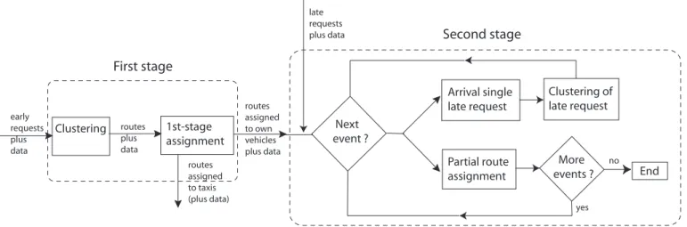
Figure 1: Schematic overview of the two-stage recourse model.
Figure 1 contains a schematic overview of the model. In the first stage, modeling today, all early requests are clustered into routes. For this purpose, a clustering heuristic is developed and described in [7]. In this heuristic, the clustering of requests is based on common locations since in paratransit trans- port some locations like hospitals and elderly homes occur frequently. After the requests have been clustered into routes, the routes are assigned to own vehicles and taxis. The assignment of routes to subcontractors (i.e., to be served by taxis) is permanent. Thus, these routes are not reconsidered tomorrow, and therefore do not appear in the second-stage problem. In contrast, the assign- ment of routes to own vehicles is preliminary since tomorrow this assignment can be changed.
The objective of the DDaPP problem is to find the assignment with minimal (expected) costs. The costs of an assignment consist of two parts: the costs of the routes assigned to a taxi today (the first-stage costs) and the expected costs of the second-stage problem in which all remaining routes and the late requests will need to be given a permanent assignment. That is, in both stages only the costs of the permanent assignments are taken into account. To find an assignment with small (expected) costs, we use a genetic algorithm described in Section 4.3.
In the second stage, modeling tomorrow, for a given first-stage assignment and given realization of the late requests, an event-driven approach is used to solve the online optimization problem. This problem is to find the minimal cost assignment of the routes assigned to own vehicles in the first stage and all late requests. Since this assignment is permanent, all assignment costs are taken into account.
Since requests need to be subcontracted at least a certain time before they start, say tsub, at the start of the day of operation all routes starting within tsub are given a permanent assignment. As time progresses, all routes starting within a time frame fromtsubare assigned permanently, and the corresponding costs are added to the total costs. Hence, at the end of the day the total costs reflect the costs of serving all routes and late requests.
There are two types of events:
• the arrival of a late request, with stochastic interarrival times, and
• part of the routes are given a permanent assignment, with deterministic interarrival times.
Every time a late requests arrives, immediately an attempt is made to com- bine the request with routes having a preliminary assignment. Hence, an online decision is made. Since it would be too time-consuming to use the clustering heuristic of the first stage, it has been modified. The idea is to split the routes (only those with a preliminary assignment) into subgroups based on common locations. Throughout the the day of operation these subgroups are maintained and updated if necessary. As soon as a late request arrives, it is attempted to be combined with routes from a subgroup which have the same origin or des- tination. In Section 4.1, the modified clustering heuristic will be described in
more detail.
Unlike the clustering in which time is measured continuously, to assign routes to vehicles time is discretized in periods of equal length, say lper. At the be- ginning of every period, the assignment heuristic, described in Section 4.2, is used to give part of the routes a permanent assignment. These routes start withintsub and tsub+lper. Routes starting earlier already have a permanent assignment and routes starting even later will be taken into account (but not the late requests which have not arrived yet).
Notice that until the first late request arrives, all routes which need to be given a permanent assignment, are assigned to an own vehicle. Furthermore, since all late requests are assumed to be known at leasttsub+lper before they start, an attempt can be made to combine a late request before it is given a permanent assignment.
4 Solution methods
In Section 4.1, we present the heuristic to combine a single late request with routes having only a preliminary assignment. This heuristic is based on the one used in the first stage to cluster the early requests with each other. Hence, the heuristic is based on the data of individual requests. To allow application in the second stage, the routes therefore are reformulated as requests. Moreover, a modification of the original heuristic is necessary since otherwise combining every single late request with a group of (reformulated) routes would be too time-consuming.
Section 4.2 contains the heuristic to give part of the routes a permanent assignment. This heuristic originates from the one developed and described in [7]. Modifications have been made since now only part of the routes are given a permanent assignment, not all.
A short description of the genetic algorithm used to solve the recourse model can be found in Section 4.3. This algorithm is very similar to the one used to solve the model of the simplified problem in which the late requests are assumed to be known at beginning of tomorrow [7]. In fact, only the cost function (fitness function) is different. Hence, in Section 4.3 the genetic algorithm is described briefly, with an extensive description of the cost function. For details we refer the interested reader to [7] or to [10, 16] for information on genetic algorithms in general.
4.1 Modified clustering heuristic
The input of the modified heuristic consists of one late request and the set of (reformulated) routes which only have a preliminary assignment. Routes having a permanent assignment are not taken into account, since they are not allowed to be changed anymore.
Before the heuristic starts, a preprocessing step is performed: either sub- groups are created (only the first time) or updated. To create subgroups all
routes are divided such that the routes in a subgroup have their origin or des- tination in common. Routes which have no location in common are put in the so-called rest group. Updating subgroups consists of removing routes which have been assigned permanently. If a subgroup consists of a single route, the route is moved to the rest group and the subgroup is deleted. Thus, all sub- groups, except the rest group, consist of at least two routes. If possible, new subgroups are created containing at least one route just moved to the rest group.
For example, a route belongs to a subgroup with equal destinations. All other routes in the subgroup have been given a permanent assignment, and hence the route is moved to the rest group. In there, a route exists which has the same origin, and hence both routes form a new subgroup.
After the subgroups have been created or updated, we try to combine the late request. First, the an appropriate subgroup is searched for: one for which the origin (destination) of the late request is equal to the origin (destination) of all routes in the subgroup. The routes in this subgroup are ordered based on direct ride time, since we expect routes with a long direct ride time to have a good potential to be clustered with other routes / requests. Then, in the order specified by the list, we try to combine the late request with a route from the subgroup. Of course, the clustering conditions specified in Section 2 have to be satisfied.
If the late request is combined with an existing route, the data of the route is updated. This data consists of an indicator of the vehicle type (a van route or not), the three different cost parameters of serving the route with a car, van, and taxi, respectively, and the time periods in which the route starts and ends.
If the clustering is not successful, the request is transformed into a route, and the subgroups need to be updated. We distinguish three cases. First, if the investigated subgroup is not the rest group, the newly formed route is added to that subgroup. In the second case, in the rest group a route with the same origin (or destination) as the late request can be found. Both routes form a new subgroup and are deleted from the rest group. In the last case, the newly formed route ends up in the rest group since there are no other routes in there which have the same origin or destination.
4.2 Modified assignment heuristic
For the assignment of routes to vehicles we use the cost-based heuristic devel- oped in [7], with minor modifications outlined below. The heuristic produces good results and is fast, which is important since it is applied many times.
Two modifications to the original heuristic are necessary since now only part of the routes are given a permanent assignment. First, some routes already have a permanent assignment so that the number of available own vehicles needs to be decreased accordingly. Second, routes starting later than tsub+lper from now are not given a permanent assignment, but are taken into account if they start within a certain look-ahead periodp. For example, to decide about a route starting at 10 AM it is not necessary to consider routes starting in the evening.
In Section 5.2, we will decide on the length of the look-ahead period. Routes
starting later than tsub +lper +p from now will be ignored in the modified assignment heuristic.
4.3 Genetic algorithm
In the Genetic Algorithm (GA), the standard 0-1 binary representation is used to describe the individuals of the population. Each population member consists ofn bits, withnthe number of routes in the first stage. The binary variables indicate whether the corresponding route is assigned to a subcontractor (one) or served with an own vehicle (zero). There are 2npossible distinct solutions, which are not all feasible. A solution is said to be infeasible if in any time period more own vehicles of a particular type are needed than there are available. Infeasible solutions are discarded and will never enter the population.
The cost function (fitness function) is equal to the expected costs of the first-stage problem: the costs of assigning the early requests to subcontractors plus the expected costs of the second-stage problem. To estimate the latter a sample of realizations of the late requests is drawn, and for each realization the costs of assigning the remaining early requests and all late requests to own vehicles and taxis are calculated. The average costs of all realizations give the estimated costs of the second-stage problem.
To solve the second-stage problem for a particular realization and given first-stage solution, the event-driven heuristic is applied, in which the modified clustering and assignment heuristic are called many times. For a large sample size it will take much time to calculate the estimated costs of an individual.
However, using only a small number of realizations might give a bad approx- imation of the expected costs of the second-stage problem, and thus also of those of the first-stage problem. In Section 5.2 we will decide on the number of realizations and give confidence intervals for the estimated costs of various solutions.
To select parents the binary tournament selection method is used in which two individuals from the population are chosen randomly. The cheapest (i.e., fittest) individual is chosen as the first parent. The second parent is obtained in the same manner.
Children are created by the one-point crossover procedure. In this procedure, a crossover point is selected randomly. The first child obtains the bits to the left of this point from the first parent, and the remaining bits from the second parent, and vice versa to create a second child.
After the crossover procedure two random bits in each child are mutated.
Then, each child is checked for feasibility which is not easy since the non-van routes can be assigned to a car or to a van. We have chosen to perform a simple check for feasibility which never accepts an infeasible solution, but might reject a (just) feasible solution. In this feasibility check, we first examine whether there are enough own vehicles (regardless of the type) to serve all routes which have not been subcontracted, and whether all van routes can be served by vans.
As soon as one of these conditions fails, the child is infeasible. If both conditions are satisfied, and all non-van routes can be served by cars, the child is feasible.
In the remaining case we try to assign some non-van routes to vans to create a feasible assignment. If this is not successful, we regard the child as infeasible.
Finally, the children replace the two most expensive population members, but only if the estimated costs of the child are lower. Duplicate solutions are not allowed to enter the population.
The selection-reproduction-evaluation-replacement cycle ends when a given number of non-duplicate, feasible children has been generated.
5 Numerical experiments
In this section, we describe our numerical experiments and the results: in Section 5.1 we describe how the data instances are generated and in Section 5.2 the parameter setting of our solution method is discussed. Furthermore, the effect of taking into account the late requests is presented in Section 5.3, and the effect of clustering the requests into routes in Section 5.4. In [7], we studied a similar problem in which we assume all late requests to be revealed early tomorrow morning instead of gradually during that day. A comparison of the DDaPP problem to this problem, called the simplified problem below, can be found in Section 5.5.
5.1 Data
All data instances used for the experiments are exactly equal to those used for the simplified problem, so that the results can be compared. All instances are randomly generated (using common random numbers) and contain 50 early requests. The number of late requests varies between 5 and 25.
pickup time 7 – 10 AM capacity car 3
delivery time until noon capacity van 6
number of customers per request 1 tsub 1 hour
fixed fee subcontracting 3 lper 15 minutes
Table 1: Part of the data of the instances
Table 1 contains part of the data of our instances. Furthermore, the ca- pacities of the vehicles do not depend on the customer type. The chance on a wheelchair customer is equal to 0.125. All locations lie on a 7×7-grid and have an equal chance of being chosen, except for two special locations, e.g., hospitals, which have a higher chance, varying between 0.05 and 0.3. The costs of serving a request/route for one grid unit with a car, van, and taxi are respectively 0.8, 1, and 1. Subcontracting tomorrow is 20% more expensive than today. Until 10 AM, 10 cars are available, thereafter 4, and all day 3 vans are available. All vehicles have a speed of 8 grid units per hour.
The experiments are performed on a 2.4 Ghz Intel Pentium 4. With the parameter setting of Section 5.2, the running time of the GA varies between 55 and 145 minutes of CPU time per instance.
5.2 Parameter setting
In the modified assignment heuristic a look-ahead period is used to determine which routes with a preliminary assignment are taken into account when giving part of the routes a permanent assignment. Various tests show that the length of this period (within a range of 1–3 hours) has very limited influence on the results: the estimated costs of a solution vary little, and also the running time of the GA remains almost the same. The results presented below are obtained with a look-ahead period of 2 hours: the maximal length of a request plus 30 minutes extra.
The population size of the GA is set equal to 30 members. For the simplified problem [7] we have experimented with random and structured initial population members, and observed that the latter lead to faster convergence of the GA to a good solution. Since the DDaPP problem is very closely related, we use here structured initial population members as well. These members are obtained by reducing the number of available own vehicles for certain time periods, or by setting a maximum on the number of routes that are allowed to be served with an own vehicle, or by doing both. That is, a structured initial solution reserves capacity today to be able to serve requests that become known tomorrow. A different setting to reserve capacity is used for each population member, e.g., for one member at most 90% of the routes are allowed to be served with own vehicles and for an other at most 50%. Since duplicate solutions are not allowed to enter the population, a solution is randomly generated if two structured initial solutions are the same. To construct such a solution routes are chosen randomly and assigned to own vehicles up to the available number for each vehicle type.
The GA stops after generating 500 non-duplicate feasible children. Based on tests with various instances, it appears that beyond this number the solution improves only marginally. Furthermore, for the simplified problem the stopping criterion was also set at 500 generated children, which gives a fair comparison.
To determine the sample size, we construct a confidence interval for the estimated costs of the best solution found. In Table 2, we have listed for four different instances the estimated costs of the solution and the 95% confidence interval when 200 realizations are used. Since the length of the interval is less than 2% for all four instances, which we think is reasonable, we set the sample size equal to 200 realizations.
Est. costs Lower bound Upper bound Length (in %)
262.37 260.32 264.42 1.57
354.71 351.56 357.85 1.79
279.22 276.76 281.69 1.78
215.98 213.85 218.11 1.99
Table 2: The estimated costs of the GA solution and the 95% confidence interval, for four different instances.
Besides the sample size, also the randomness of the genetic algorithm itself influences the quality of the results. Since the GA is a heuristic, good solutions
may not always be found. To test this effect, we ran the algorithm 10 times on the same instance. As we found that the estimated costs vary only by 1.33%, we conclude that the algorithm consistently finds solutions of similar quality.
5.3 Late requests
To determine the effect of taking into account the late requests (by using a two- stage recourse model), we introduce the GA solution and the myopic solution.
The first is the best solution found of the two-stage recourse model. The latter is the solution of the myopic model in which the probabilistic information on the late requests is ignored. That is, the myopic solution is obtained by clustering the early requests and assigning the obtained routes to vehicles by use of the original assignment heuristic (see [7]). To be able to compare both solutions, the ‘true’ estimated costs of the myopic solution are calculated by evaluating the solution in the recourse model: for each realization the second-stage problem is solved and the average second-stage costs plus the first-stage costs give the estimated costs of the solution.
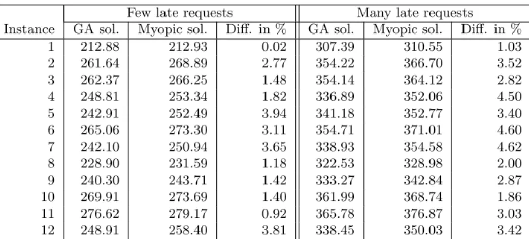
For a good comparison of both models (myopic and recourse model) we have generated 12 instances which are solved twice: once with few (5 – 10) late requests, and once with many (20 – 25) late requests. Since the early requests are the same for each variant, by definition the myopic solution is the same for few and many late requests, only the estimated costs are different. For each instance, the estimated costs of the GA solution and the myopic solution are calculated, both with few and many late requests. Furthermore, the relative difference between the estimated costs of the GA and myopic solution is determined.
Few late requests Many late requests Instance GA sol. Myopic sol. Diff. in % GA sol. Myopic sol. Diff. in %
1 212.88 212.93 0.02 307.39 310.55 1.03
2 261.64 268.89 2.77 354.22 366.70 3.52
3 262.37 266.25 1.48 354.14 364.12 2.82
4 248.81 253.34 1.82 336.89 352.06 4.50
5 242.91 252.49 3.94 341.18 352.77 3.40
6 265.06 273.30 3.11 354.71 371.01 4.60
7 242.10 250.94 3.65 338.93 354.58 4.62
8 228.90 231.59 1.18 322.53 328.98 2.00
9 240.30 243.71 1.42 333.27 342.84 2.87
10 269.91 273.69 1.40 361.99 368.74 1.86
11 276.62 279.17 0.92 365.78 376.87 3.03
12 248.91 258.40 3.81 338.45 350.03 3.42
Table 3: The effect of late requests on the estimated costs of the GA solution and the myopic solution.
Table 3 shows that the estimated costs of the myopic solutions are between 0% and 5% higher than those of the GA solutions. Recall that the length of the confidence interval is less than 2% for the four instances we have listed in Table
2, implying that for almost all instances the difference is significant. From now on, we will not mention this any more.
The myopic solutions simply assign as much early requests as possible to own vehicles, ignoring the late requests which become known tomorrow, and hence not reserving capacity for them. Consequently, tomorrow more requests/routes will need to be subcontracted, and since this is 20% more expensive than to- day, the estimated costs of the myopic solutions are higher than those of the GA solutions. The latter do take into account the late requests by means of probabilistic information. Hence, the GA solutions assign today more requests to subcontractors, but tomorrow less. When many late requests arise this effect should be and is almost always stronger: the difference (in %) is larger com- pared to the same instance when few late requests arise, except for instances 5 and 12.
Few late requests Many late requests
Inst. GA solution Myopic solution GA solution Myopic solution
Subcontr Subcontr Subcontr Subcontr
Cost Cost Num Cost Cost Num Cost Cost Num Cost Cost Num
1 212.88 28 3 212.93 24 3 307.39 64 8 310.55 24 3
2 261.64 93 11 268.89 65 10 354.22 125 16 366.70 65 10
3 262.37 77 9 266.25 65 9 354.14 118 14 364.12 65 9
4 248.81 68 9 253.34 46 7 336.89 74 9 352.06 46 7
5 242.91 70 8 252.49 56 8 341.18 97 12 352.77 56 8
6 265.06 93 11 273.30 64 10 354.71 128 16 371.01 64 10
7 242.10 64 7 250.94 46 7 338.93 116 14 354.58 46 7
8 228.90 62 8 231.59 49 7 322.53 92 12 328.98 49 7
9 240.30 75 10 243.71 62 9 333.27 107 14 342.84 62 9
10 269.91 86 12 273.69 78 12 361.99 122 16 368.74 78 12
11 276.62 83 11 279.17 73 10 365.78 134 17 376.87 73 10
12 248.91 92 11 258.40 67 10 338.45 94 11 350.03 67 10
Table 4: The effect of late requests on the GA solution and the myopic solution.
In Table 4, the columns cost are copied from Table 3, and the remaining columns show the first-stage costs (only those for subcontracting) and the num- ber of early requests assigned to taxis. The effect explained above is clearly demonstrated in this table: the myopic solutions assign less early requests to subcontractors, compared to the GA solutions which reserve capacity for to- morrow. When many late requests arise the effects are stronger. Except for instances 4 and 12, considerably more early requests are assigned to subcon- tractors in the GA solution, and hence the first-stage costs of the GA solution are also larger.
5.4 Clustering
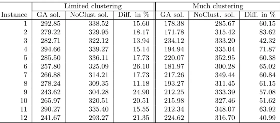
To determine the effect of clustering the requests into routes, we have con- structed NoClust solutions for comparison to the GA solutions. A NoClust
solution is obtained by applying the GA to individual requests – as opposed to clustered routes – in the first stage, and no clustering of late requests in the second stage.
Again, we have generated 12 instances each with two variants: few and many clustering possibilities, implemented by specifying the probability of a special location as 0.05 and 0.3, respectively. These probabilities hold for both the early and the late requests. The number of late requests now varies between 8 and 14. For each instance, limited and much clustering, the estimated costs of the GA and NoClust solutions are calculated, as well as their relative difference.
Limited clustering Much clustering
Instance GA sol. NoClust sol. Diff. in % GA sol. NoClust. sol. Diff. in %
1 292.85 338.52 15.60 178.38 285.67 60.15
2 279.22 329.95 18.17 171.78 315.42 83.62
3 282.71 322.12 13.94 234.12 333.20 42.32
4 294.66 339.27 15.14 194.94 335.04 71.87
5 285.50 336.11 17.73 220.07 352.95 60.38
6 257.80 325.09 26.10 181.97 300.28 65.02
7 266.88 314.21 17.73 217.26 349.44 60.84
8 278.24 309.35 11.18 193.27 311.45 61.15
9 243.62 304.28 24.90 212.25 333.39 57.08
10 265.97 320.51 20.51 215.98 327.46 51.62
11 290.27 335.40 15.55 212.34 348.07 63.92
12 241.67 293.27 21.35 224.62 316.70 40.99
Table 5: The effect of clustering on the estimated costs of the GA solution and NoClust solution.
Table 5 shows that the estimated costs of the NoClust solutions are between 11% and 84% higher than those of the GA solutions. As expected, the difference is largest when there are many clustering possibilities, although even when there are few clustering possibilities the difference in estimated costs is considerable.
5.5 DDaPP problem versus simplified problem
In this paper, we have frequently referred to an earlier paper in which we studied the simplified, but less realistic version of the DDaPP problem. In Section 5.5.1, we will show that it can be profitable to solve the DDaPP problem instead of the simplified version. Although the latter is easier to solve, the running time of its GA is larger when only few late requests arise, since in that case checking all subgroups for possible combinations takes more time than combining repeatedly a single late request, as is the case in the DDaPP problem. When many late requests arise, the running time of the GA of the simplified problem is shorter, as expected.
As already mentioned before, the main difference between both problems is the flow of information on the late requests. In Section 5.5.2, it is investigated what the benefit is (in terms of less costs) of having more information on the
late requests. That is, in the simplified problem the late requests become known early in the morning instead of during the day. Hence, more information is available on the late requests at the time decisions are to be made, which we expect to lead to better decisions with lower estimated costs.
To present the results of this section clearly, we introduce some notation. Let xD and xs be the best solution found of the DDaPP and simplified problem, respectively. Furthermore, letfD(·) andfs(·) be the cost function of the DDaPP and simplified problem, respectively. Then, for example, fD(xs) denotes the estimated costs of the best solution of the simplified problem when evaluated in the DDaPP problem.
5.5.1 Solving simplified instead of realistic problem
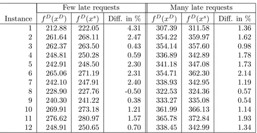
A relevant issue in practice is which problem to solve: the simplified one which presumably results in worse decisions, or the more realistic, but also more diffi- cult DDaPP problem which hopefully leads to better decisions. To answer this question, the best solution of the simplified problem is evaluated in the DDaPP problem. This gives the ‘true’ estimated costsfD(xs) which will be compared to those of the best solution of the DDaPP problemfD(xD). Besides the true estimated costs of the best solution of both problems, also the difference (in %) is determined. This difference denotes the extra costs incurred by solving the simplified instead of the more realistic DDaPP problem. The results have been calculated for the instances with few and many late requests.
Few late requests Many late requests Instance fD(xD) fD(xs) Diff. in % fD(xD) fD(xs) Diff. in %
1 212.88 222.05 4.31 307.39 311.58 1.36
2 261.64 268.11 2.47 354.22 359.97 1.62
3 262.37 263.50 0.43 354.14 357.60 0.98
4 248.81 250.28 0.59 336.89 342.89 1.78
5 242.91 248.50 2.30 341.18 347.08 1.73
6 265.06 271.19 2.31 354.71 362.30 2.14
7 242.10 247.91 2.40 338.93 342.95 1.19
8 228.90 227.76 -0.50 322.53 324.36 0.57
9 240.30 241.22 0.38 333.27 335.08 0.54
10 269.91 273.18 1.21 361.99 366.13 1.14
11 276.62 280.97 1.57 365.78 372.84 1.93
12 248.91 250.65 0.70 338.45 342.99 1.34
Table 6: The extra costs incurred by solving the simplified instead of the DDaPP problem.
Table 6 shows that for all instances, except one, it is better to solve the more realistic DDaPP problem than the simplified one. That is, the estimated costs are at most 4% higher when the simplified problem is solved instead of the more realistic and difficult DDaPP problem. Unfortunately, these results are not very
convincing, but the difference in true estimated costs of both solutions is in at least 2 out of 3 instances significant, using the confidence intervals of Table 2.
Hence, we tentatively conclude that it is profitable to solve the more realistic DDaPP problem.
5.5.2 Benefit of more information on the future
The main difference between the simplified problem and the more realistic, but also more difficult DDaPP problem is the flow of information on the late re- quests. To determine what the benefit is (in terms of less costs) of having more timely information, the comparison should not be influenced by other factors.
Unfortunately, in the DDaPP problem much more late requests are combined than in the simplified problem. This is counterintuitive, but can be easily ex- plained. In the DDaPP problem, the subgroups for clustering are updated regularly during the event-driven heuristic, while in the simplified problem they remain the same since all late requests are combined at once. This allows more combinations to be made in the DDaPP problem, decreasing the estimated costs, and hence making the comparison unfair. To correct this, the clustering heuris- tic of the simplified problem has been adjusted, but only in the second stage.
That is, besides the four subgroups based on special locations only one subgroup is used. This increases the running time considerably, but is acceptable in our view since we only use the results for comparison.
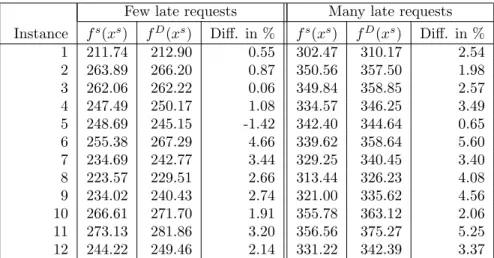
To calculate the benefit of having more information on the late requests, the best solution of the simplified problem is evaluated twice: once in the simplified problem (fs(xs)), and once in the DDaPP problem (fD(xs)). The difference (in %) between both estimated costs denotes the benefit. Again, the results are only calculated for the instances with few and many late requests.
Notice that the columnsfD(xs) of Tables 6 and 7 do not coincide sincexsis not the same. This is caused by the small adjustment of the clustering heuristic in the simplified problem.
As can be seen in Table 7, there is only one instance for which having more information on the future is not profitable, i.e., the estimated costs increase when the late requests are known early tomorrow morning instead of gradually revealed. This is probably caused by an unfortunate outcome of the heuristics.
For all other instances, the estimated costs decrease with at most 6% when more information is available on the late requests. Based on this numerical evidence, we conclude that (unrealistically) timely information on future requests would lead to slightly better decisions in the paratransit problem at hand.
6 Summary and conclusion
We have formulated the Dynamic Day-ahead Paratransit Planning problem, in which we decide day-ahead, when only part of the requests are known, which requests to subcontract and which ones to assign to own vehicles. Since already today it is known that there are not enough own vehicles to serve all requests, it
Few late requests Many late requests Instance fs(xs) fD(xs) Diff. in % fs(xs) fD(xs) Diff. in %
1 211.74 212.90 0.55 302.47 310.17 2.54
2 263.89 266.20 0.87 350.56 357.50 1.98
3 262.06 262.22 0.06 349.84 358.85 2.57
4 247.49 250.17 1.08 334.57 346.25 3.49
5 248.69 245.15 -1.42 342.40 344.64 0.65
6 255.38 267.29 4.66 339.62 358.64 5.60
7 234.69 242.77 3.44 329.25 340.45 3.40
8 223.57 229.51 2.66 313.44 326.23 4.08
9 234.02 240.43 2.74 321.00 335.62 4.56
10 266.61 271.70 1.91 355.78 363.12 2.06
11 273.13 281.86 3.20 356.56 375.27 5.25
12 244.22 249.46 2.14 331.22 342.39 3.37
Table 7: The benefit of having more information on the late requests.
can be profitable to make this decision. The focus is on the clustering of requests into routes, and on coping with the uncertainty due to the late requests which are gradually revealed.
In the non-standard two-stage recourse model we have developed, the first stage consists of two optimization problems to be solved consecutively. More- over, the dynamic second-stage problem is modeled as an online optimization problem while typically it consists of a (mixed-integer) linear programming prob- lem. As far as we know, no such combination of ideas from stochastic program- ming and online optimization has been made before. By introducing this model, we present an alternative for the commonly used deterministic models. In this alternative, a realistic look-ahead feature is incorporated as suggested by several other studies (e.g. [2, 5]).
Our model and solution method are flexible and can easily be adjusted, e.g., to incorporate various numbers of customers, to have different characteristics for the early and late requests, or to include events like canceled requests and vehicle breakdowns.
The results are promising. Clustering of requests is very profitable: the esti- mated costs are much lower compared to the same instances when the individual requests are considered. Taking into account the late requests decreases the es- timated costs on average with 2.5%. CPU times are, however, rather large. We will conduct a follow-up study to decrease CPU times.
In an earlier paper we studied a simplified version of the DDaPP problem in which all late requests are revealed early tomorrow morning instead of gradu- ally during the day. It is shown that having more timely information on future requests leads in general to better decisions with lower estimated costs. Further- more, for many test instances it appears to be profitable to solve the realistic problem instead of the simplified one. Unfortunately, these results are not very convincing and further research is needed.
References
[1] S. Albers. Online algorithms: A survey. Mathematical Programming, 97(1- 2):3–26, 2003.
[2] A. Attanasio, J.-F. Cordeau, G. Ghiani, and G. Laporte. Parallel tabu search heuristics for the dynamic multi-vehicle dial-a-ride problem.Parallel Computing, 30:377–387, 2004.
[3] J.R. Birge and F. Louveaux. Introduction to Stochastic Programming.
Springer-Verlag, New York, 1997.
[4] R. Bornd¨orfer, M. Gr¨otschel, F. Klostermeier, and C. K¨uttner. Telebus Berlin: Vehicle scheduling in a dial-a-ride system. ZIB Report 97-23, April 1997.
[5] J.-F. Cordeau and G. Laporte. The dial-a-ride problem (DARP): Variants, modeling issues and algorithms. Quarterly Journal of the Belgian, French and Italian Operations Research Societies, 1:89–101, 2003.
[6] J.-F. Cordeau and G. Laporte. A tabu search heuristic for the static multi- vehicle dial-a-ride problem.Transportation Research Part B, 37(6):579–594, 2003.
[7] M.L.A.G. Cremers, W.K. Klein Haneveld, and M.H. van der Vlerk. A two- stage model for a day-ahead paratransit planning problem.http://mally.
eco.rug.nl/papers/DaPP.htm.
[8] J. Desrosiers, Y. Dumas, F. Soumis, S. Taillefer, and D. Villeneuve. An algorithm for mini-clustering in handicapped transport. Les Cahiers du GERAD, G-91-02, ´Ecole des Hautes ´Etudes Commerciales, Montr´eal, 1991.
[9] M. Diana and M.M. Dessouky. A new regret insertion heuristic for solving large-scale dial-a-ride problems with time windows. Transportation Re- search Part B, 38:539–557, 2004.
[10] D.E. Goldberg. Genetic Algorithms in Search, Optimization, and Machine Learning. Addison-Wesley, 1989.
[11] M. Gr¨otschel, S.O. Krumke, J. Rambau, T. Winter, and U.T. Zimmer- mann. Combinatorial online optimization in real time. In Martin Gr¨otschel, Sven O. Krumke, and J¨org Rambau, editors,Online Optimization of Large Scale Systems, pages 679–704. Springer, 2001.
[12] I. Ioachim, J. Desrosiers, Y. Dumas, M.S. Solomon, and D. Villeneuve. A request clustering algorithm for door-to-door handicapped transportation.
Transportation Science, 29:63–78, 1995.
[13] R.M. Jørgensen, J. Larsen, and K.B. Bergvinsdottir. Solving the dial-a- ride problem using genetic algorithms.Journal of the Operational Research Society, 58:1321–1331, 2007.
[14] P. Kall and J. Mayer. Stochastic Linear Programming: Models, Theory, and Computation. Kluwer Academic Publishers, New York, 2005.
[15] O.B.G. Madsen, H.F. Ravn, and J.M. Rygaard. A heuristic algorithm for a dial-a-ride problem with time windows, multiple capacities, and multiple objectives. Annals of Operations Research, 60:193–208, 1995.
[16] C.R. Reeves. Modern Heuristic Techniques for Combinatorial Problems.
Blackwell Scientific, 1993.
[17] A. Ruszczynski and A. Shapiro, editors. Stochastic Programming, vol- ume 10 of Handbooks in Operations Research and Management Science.
North-Holland, 2003.
[18] P. Toth and D. Vigo. Heuristic algorithms for the handicapped persons transportation problem. Transportation Science, 31(1):60–71, 1997.
[19] K.I. Wong and M.G.H. Bell. Solution of the dial-a-ride problem with multi-dimensional capacity constraints. International Transactions in Op- erational Research, 13:195–208, 2006.