transformations and
bosonisation of granular fermionic systems
I n a u g u r a l - D i s s e r t a t i o n zur
Erlangung des Doktorgrades
der Mathematisch-Naturwissenschaftlichen Fakult¨ at der Universit¨ at zu K¨ oln
vorgelegt von Jakob M¨ uller-Hill
aus K¨ oln
2009
Prof. Dr. Hans-Peter Nilles
Tag der m¨ undlichen Pr¨ ufung: 26 Juni 2009
Zusammenfassung
Die vorliegende Arbeit besteht aus zwei Teilen. Der erste Teil besch¨ aftigt sich mit hyperbolischen Hubbard-Stratonovich-Transformationen. Solche Transformationen werden z.B. im Bereich der ungeordneten Elektronensys- teme ben¨ otigt, um nichtlineare Sigma-Modelle herzuleiten, die das Niederen- ergieverhalten dieser Systeme beschreiben. Der mathematische Status hy- perbolischer Hubbard-Stratonovich-Transformationen vom Pruisken-Sch¨ afer- Typ war lange ungekl¨ art. K¨ urzlich wurden zwei Spezialf¨ alle, n¨ amlich die pseudounit¨ arer und pseudoorthogonaler Symmetrie, bewiesen [10, 11, 12].
In dieser Arbeit wird nun der Fall einer allgemeinen (im wesentlichen halb- einfachen) Symmetriegruppe bewiesen. Der Beweis ist anschaulich und zeigt explizit den Zusammenhang mit Standard-Gauß-Integralen.
Im zweiten Teil wird eine eine neuartige Methode entwickelt, um wech- selwirkende granular fermionische Systeme zu bosonisieren. Die Methode ist nicht mit der bekannten Bosonisierung (1 + 1)-dimensionaler Systeme verwandt, sondern eher im Bereich der koh¨ arenten Zust¨ ande anzusiedeln.
Ein Zugang ist, die Grassmann-Pfadintegraldarstellung einer großkanon-
ischen Zustandssumme durch mehrfache Anwendung der Colour-Flavour-
Transformation in eine Form zu bringen, welche die Eliminierung der Grass-
mannvariablen erlaubt. Das Resulat ist ein Pfadintegral in generalisierten
koh¨ arenten Zust¨ anden mit speziellen Randbedingungen.
Abstract
The present work consists of two parts. The first part deals with hyperbolic Hubbard-Stratonovich transformations. Such transformations are used to derive non-linear sigma models that describe the low energy behaviour of disordered electron systems. For a long time the mathematical status of hyperbolic Hubbard-Stratonovich transformations of Pruisken-Sch¨ afer type remained unclear. Only recently the two special cases of pseudounitary and pseudoorthogonal symmetry were proven [10, 11, 12]. In this thesis we prove the transformation for a general (essentially semisimple) symmetry group.
The proof is descriptive and shows explicitly the connection to the standard Gaussian integrals.
In the second part we develop a novel method to bosonise granular fermionic systems. The method is related to the method of coherent states.
In particular it is not based on the well known bosonisation of (1 + 1)-
dimensional systems. One approach is to use the colour-flavour transfor-
mation to transform the Grassmann path integral representation of a grand
canonical partition function in a way that allows to eliminate the Grassmann
variables. The result is a path integral in generalised coherent states with
special boundary conditions.
Introduction v 1 Hyperbolic Hubbard-Stratonovich transformations 1
1.1 Motivation . . . . 1
1.2 Two dimensional example . . . . 3
1.3 General setting and theorem . . . . 9
1.4 Proof of the theorem . . . . 11
1.5 Examples . . . . 33
2 Bosonisation of granular fermionic systems 37 2.1 Granular bosonisation via colour-flavour transformation . . . 37
2.2 Fock space approach to granular bosonisation . . . . 44
2.3 Contributions of fluctuations . . . . 46
Conclusion 57 A Techniques needed in chapter one 59 A.1 Basic constructions and useful relations . . . . 59
A.2 Three additional arguments . . . . 64
B Techniques needed in chapter two 67 B.1 Canonical transformations of fermionic Fock space . . . . 67
B.2 Fermionic Howe pairs and colour-flavour transformation . . . 70
Bibliography 77
iii
To obtain an adequate description of a physical system, and to compute quantities of interest, it is often necessary to replace the microscopic degrees of freedom of the system by physically more relevant ‘collective’ degrees of freedom. Two prominent methods to introduce collective variables in the field of many particle physics are Hubbard-Stratonovich transformations and bosonisation. In this work we discuss special variants of both methods. The first part of this work clarifies the mathematical status of a class of hyper- bolic Hubbard-Stratonovich transformations, whereas in the second part a new kind of bosonisation is developed. The focus of this work is rather on methodology than on applications.
Let us start with a more detailed introduction to the first part of the thesis. First, we explain where hyperbolic Hubbard-Stratonovich transfor- mations are commonly used. A natural area of application of hyperbolic Hubbard-Stratonovich transformations are disordered electron systems [1]
and their description in the form of non-compact non-linear sigma models.
The corresponding formalism was pioneered by Wegner [3], Sch¨ afer & Weg- ner [4], and Pruisken & Sch¨ afer [5]. Efetov [2] developed the more rigorous supersymmetry method, which avoids the use of the replica trick, to derive (supersymmetric) non-linear sigma models. The supersymmetry method has a wide range of applications [15]. Examples are the description of single electron motion in a disordered or chaotic mesoscopic system [16], chaotic scattering [6], and Anderson localisation [17]. Traditional derivations of non-linear sigma models in the supersymmetry formalism rely crucially on hyperbolic Hubbard-Stratonovich transformations. To describe what hy- perbolic Hubbard-Stratonovich transformations are we briefly review the case of (mathematically trivial) ordinary Hubbard-Stratonovich transfor- mations. These transformations are frequently used throughout condensed matter field theory. From a mathematical point of view such a Hubbard- Stratonovich transformation consists of applying a Gaussian integral formula backwards, i.e., introducing additional integrations. Such a scheme converts a quartic interaction term in the original variables into a quadratic term coupled linearly to the newly introduced integration variables. The word
‘hyperbolic’ indicates a non-compact symmetry group of the original sys-
v
tem. In such a situation the standard Gaussian integral formula cannot be applied due to issues of convergence.
1A solution to this problem was given by Sch¨ afer and Wegner [4]. They found a contour of integration for which the Gaussian integral formula holds and convergence is guaranteed. Never- theless the majority of the physics community uses a different contour sug- gested by Pruisken and Sch¨ afer [5] which, in contrast to the Sch¨ afer-Wegner solution, preserves the full symmetry of the original system. However, un- til recently there existed no proof of the validity of the Pruisken-Sch¨ afer transformation. The main difficulty is that the Pruisken-Sch¨ afer domain has a boundary. This prevents an easy proof similar to the standard Gaus- sian integral and to the Sch¨ afer-Wegner domain. Recently, several cases of the Pruisken-Sch¨ afer transformation have been made rigorous by Fyodorov, Wei and Zirnbauer. Fyodorov [10] gave a proof for pseudounitary symmetry by using methods of semiclassical exactness. After that Fyodorov and Wei [11] proved a variant of the Pruisken-Sch¨ afer transformation for the case of O(1, 1) and O(2, 1) symmetry by direct calculation, and proposed a re- sult for the full O(p, q) case. They conjectured that the Gaussian integral decomposes into differerent parts that have to be weighted with certain al- ternating sign factors to obtain the right result. This conjecture indicates that the Pruisken-Sch¨ afer transformation for the pseudoorthogonal case is not correct in its original form. Finally Fyodorov, Wei and Zirnbauer [12]
proved the conjecture by reducing the calculation to the O(1, 1) case and showing explicitly that all relevant boundary contributions vanish.
The motivation for our work is twofold. First, we want to obtain a bet- ter understanding of the somewhat mysterious alternating sign factors that appear in the O(p, q) case, and second, we want to generalise the trans- formation to more symmetry classes. The basic idea we follow is that in some sense, the Pruisken-Sch¨ afer domain should be a deformation of the standard Gaussian domain. The problem of the boundary of the Pruisken- Sch¨ afer contour is overcome by extending it, such that the integral remains unchanged and the boundary is moved to infinity. This leads to a proof of a variant of the Pruisken-Sch¨ afer transformation for a general symmetry group. The proof shows that it is possible to deform the Pruisken-Sch¨ afer integration contour into the standard Gaussian contour without changing the value of the integral. Actually the same can be done with the Sch¨ afer- Wegner contour.
The structure of chapter one is as follows: First we give a more detailed motivation and a description of the convergence problems one encounters when applying the Gaussian integral in case of a non-compact symmetry.
Next we discuss a two dimensional example that gives a road map for the general proof. Then we state our result and give its proof. Finally we show how to obtain the pseudounitary and pseudoorthogonal cases as special cases
1
A detailed discussion of this issue is given at the beginning of chapter one.
of the general result.
The second part of this work explores a new method of bosonisation of granular fermionic systems. The terminology ‘granular fermionic’ indi- cates the structure of a fermionic vector model. In the following we list some examples: The well known Gross-Neveu models [22] and all fermionic models having an orbital degeneracy are in this class. An exactly solvable toy model is the Lipkin-Meshkov-Glick model [21]. A more complicated example is the many orbital generalisation of the Hubbard-model. A class of models which is currently intensively studied in mesoscopic physics are arrays of quantum dots or granular metals [24]. Each quantum dot is de- scribed by the universal Hamiltonian, which has a large orbital degeneracy [23]. Note that granularity, or equivalently large orbital degeneracy, implies the existence of a natural large N limit. Such large N limits are classical limits. For Gross-Neveu models this was investigated by Berezin [33] and for a much larger class of models by Yaffe [34]. In our work we will restrict ourselves to discrete (lattice) models that have either orthogonal, unitary or unitary symplectic symmetry. This contains all relevant possibilities for the universal Hamiltonian [23]. The term ‘bosonisation’ does not refer to the well known (non) Abelian bosonisation [19], which is limited to (1 + 1) dimensional models, but rather to the natural geometric approach through generalised coherent state path integrals [35, 36].
2It is interesting to note that these path integrals lead to a generalised Holstein-Primakoff transfor- mation [18].
The restriction to granular fermionic systems with a classical Lie group as symmetry group gives access to powerful results from the theory of Howe dual pairs [27, 28]. One important tool that relies on the theory of Howe dual pairs is the colour-flavour transformation [29, 30]. Within our method we put the available structure to use in the calculation of the grand canonical partition function of a granular fermionic system. The result we obtain is a path integral representation of the grand canonical partition function of the granular fermionic system in terms of bosonic, i.e. commuting variables. The representation is essentially a path integral in generalised coherent states with certain boundary conditions. However, we cannot apply generalised coherent states directly in this context, since this would yield a path integral only for a subspace of Fock space.
The structure of the second part is as follows: We consecutively discuss two different derivations of the bosonic path integral representation of the grand canonical partition function. Furthermore we calculate the contribu- tion of fluctuations in the semiclassical limit in terms of classical quantities.
2
There have also been attempts to use coherent state path integrals for loop groups
[20] to bosonise (1 + 1) dimensional models.
Hyperbolic
Hubbard-Stratonovich transformations
1.1 Motivation
Non-compact non-linear sigma models are important and extensively used tools in the study of disordered electron systems. As mentioned in the introduction, the corresponding formalism was pioneered by Wegner [3], Sch¨ afer & Wegner [4], and Pruisken & Sch¨ afer [5]. Shortly afterwards Efetov [2] improved the formalism. He developed the supersymmetry method to derive non-linear sigma models. Many applications of the supersymmetry method can be found in the textbook by Efetov [15].
There are different ways to derive non-linear sigma models from micro- scopic models, for an introduction see [8]. The traditional approach is to use a Hubbard-Stratonovich transformation, i.e., a transformation of the form
c
0e
−TrA2= Z
D
e
−TrQ2−2iTrQA|dQ| , (1.1) where c
0∈ R . We leave the domain of integration D unspecified for now.
|dQ| denotes Lebesgue measure of a normed vector space.
Let us discuss the case of pseudoorthogonal symmetry O(p, q) as an ex- ample. Then A is given by A
ij= P
Na=1
Φ
a,iΦ
a,js
jjwith s = Diag( 1
p, − 1
q) and Φ
a,j∈ R. The Φ
a,jrepresent the microscopic degrees of freedom. Us- ing equation (1.1) and integrating out φ gives a description in terms of the effective degrees of freedom Q. Thus the task is to find a domain of integration D for which identity (1.1) holds and the term exp(−2i Tr QA) stays bounded. The latter allows to perform the Φ integrals after applying identity (1.1). Note that the real matrices A fulfil the symmetry relation A = sA
ts. A naive choice of the domain of integration D to keep the term
1
exp(−2i Tr QA) bounded would be the domain of all real matrices satisfy- ing Q = sQ
ts. This choice of D is not valid since then the quadratic form Tr Q
2= Tr QsQ
ts is of indefinite sign.
Sch¨ afer and Wegner [4] found a domain D=SW, and gave a proof that it solves the problem. Nonetheless another domain D=PS was proposed in later work by Pruisken and Sch¨ afer [5]. Until recently the mathematical status of identity (1.1) for D=PS was unclear. The main difficulty in proving identity (1.1) for D=PS is that the PS domain has a boundary. This prevents an easy proof by completing the square and shifting the contour as is possible for the standard Gauss integral and for the SW domain. Nevertheless the PS domain was used in most applications worked out by the mesoscopic physics community. The reason might be that it inherits the full symmetry of the domain of A matrices.
Recently Fyodorov, Wei and Zirnbauer [10, 11, 12] proved special cases of the Pruisken-Sch¨ afer transformation.
In the following we state the result for the O(p, q) case that was obtained in [12]. Choose D as the subspace of matrices Q = sQ
ts that can be diago- nalised by an element of O(p, q). The domain D can be seen as the union of
p+q p
subdomains D
σ. The domains D
σare labeled as follows. Up to a set of measure zero Q ∈ D has p ‘space-like’ eigenvectors {v
i}
i≤pwith v
itsv
i> 0 and q ‘time-like’ eigenvectors {v
i}
q<i≤pwith v
itsv
i< 0. Again up to a set of measure zero in D, the eigenvalues of Q can be arranged in decreasing order. We translate this ordered sequence into a binary sequence by writing the symbol ‘•’ for space-like and ‘◦’ for time-like eigenvalues.
1Furthermore, let
|dQ| = Y
i≤j
dQ
ij(1.2)
denote flat integration measure on all domains D
σ, and let sgn(σ) be the parity of the number of transpositions • ↔ ◦ needed to reduce the binary sequence σ to the extremal form σ
0= • · · · • ◦ · · · ◦. Then the following theorem [12] holds:
Theorem 1.1. There exists some choice of cutoff function Q 7→ χ
(Q) (con- verging pointwise to unity as → 0), and a unique choice of sign function σ → sgn(σ) ∈ {±1} and a constant C
p,qsuch that
C
p,qlim
→0
X
σ
sgn(σ) Z
Dσ
e
−TrQ2−2iTrAQχ
(Q)|dQ| = e
−TrA2(1.3) holds true for all matrices A = sA
ts with the positivity property As > 0.
The alternating sign factor was already conjectured in [11]. Note that in the large N limit only one D
σcontributes to the results. Therefore earlier
1
The properties of the domains D
σare discussed in more detail in [12].
works using (1.3) without the alternating sign lead to correct results in the large N limit.
In this chapter we show a variant of theorem 1.1 for a general symmetry group. The proof shows that it is possible to deform the Pruisken-Sch¨ afer (PS) integration contour into the standard Gaussian contour without chang- ing the value of the integral. Actually the same can be done with the Sch¨ afer- Wegner (SW) contour. The problem of the boundary of PS is overcome by extending the PS domain in a way that leaves the integral unchanged and moves the boundary to infinity. The proof also demonstrates the origin of the alternating sign factors in equation 1.3
For convenience of the reader, the main ideas of the proof are first il- lustrated in a simple two dimensional example. Then we state the general results and give their proof. Finally some applications are discussed. In particular, it is discussed how the cases of pseudounitary and orthogonal symmetry fit into the general setting.
1.2 Two dimensional example
As a first step towards a general theorem of hyperbolic Hubbard-Stratonovich transformations, we discuss a two dimensional example. In this simplified setting the general result and main ideas of its proof can be nicely illustrated.
First we have to fix the setting. Let {e
1, e
2} be a basis of C
2and dq
i(e
j) = δ
ij. D denotes the parametrisation of a two dimensional surface in C
2and dq
1∧ dq
2is a holomorphic two form on C
2. Now consider the simple Gaussian type integral identity
Z
D
e
−q21+q22−2ia1q1+2ia2q2dq
1∧ dq
2= iπe
−a21+a22. (1.4) At this stage a
1and a
2may be arbitrary complex numbers. In the following we discuss different parametrisations of domains of integration D for which the identity holds. Eventually this requires imposing additional restrictions on a
1and a
2. Since we are integrating differential forms, the domains of integration must have an (inner) orientation. Note that we discern between italic D and non italic D. The former denotes the parametrisation of the domain D.
Euclidean domain of integration
Obviously identity (1.4) holds for the standard Euclidean domain of inte- gration
Euclid : R
2→ C
2(r, s) 7→ r e
1+ is e
2.
ie
2e
1Figure 1.1: Standard Euclidean domain of integration.
e
1ie
1ie
2Figure 1.2: Sch¨ afer-Wegner domain of integration.
Here the orientation comes from choosing an orientation on the domain of definition R
2and declaring Euclid to be orientation preserving. Note that the orientation of the two other domains of integration, which we discuss be- low, will be choosen in the same way. The orientation of Euclid is indicated by a sense of circulation in figure 1.1.
Sch¨ afer-Wegner domain of integration
Demanding that a
i∈ R and that a
1> a
2≥ 0, it can be checked by direct calculation that identity (1.4) also holds for the Sch¨ afer-Wegner family of domains of integration, which is given by
SW : R
2→ C
2(r, s) 7→ r e
1− ib cosh(s) e
1− ib sinh(s) e
2, where b > 0.
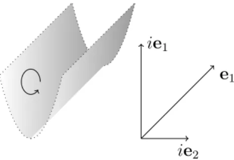
Pruisken-Sch¨ afer domain of integration The Pruisken-Sch¨ afer domain is given by
P S : R
2→ R
2(r, s) 7→ r cosh(s) e
1+ r sinh(s) e
2. (1.5)
e
1e
2Figure 1.3: Pruisken-Sch¨ afer domain of integration. The orientation is in- duced by the parametrisation (1.5).
Identity (1.4) holds for D = P S only in a regularised form. For |a
1| > |a
2| and χ (~ q) = exp(−q
22) it can be checked by direct calculation that
→0
lim Z
D
e
−q12+q22−2ia1q1+2ia2q2χ
(q)dq
1∧ dq
2= iπe
−a21+a22(1.6) holds.
Note that by introducing a Minkowski scalar product B(~a, ~ q) = a
1q
1− a
2q
2with ~a = (a
1, a
2)
tand ~ q = (q
1, q
2)
t, (1.6) can be rewritten to
→0
lim Z
D
e
−B(~q,~q)−2iB(~a,~q)χ (~ q)dq = iπe
−B(~a,~a). (1.7) Here we have used dq := dq
1∧ dq
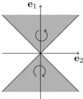
2. B has an O(1, 1) symmetry group, acting on R
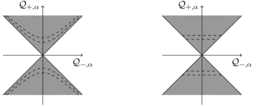
2. The Pruisken-Sch¨ afer domain of integration is invariant under the action of the group. In this case also the domain of ~a for which (1.6) holds has this invariance. Both domains (for ~a and ~ q) are given by forward and backward lightcones as depicted in figure 1.3, or, put differently, by all timelike vectors (B(~a, ~a) > 0 and B (~ q, ~ q) > 0).
Moreover, in order for (1.6) to hold it is important that the upper and lower cone (see figure 1.3) have opposite orientations. If one wants to inte- grate Lebesgue measure |dq| rather than a differential form, (1.6) has to be modified accordingly to a difference of integrals. Defining
g(~ q, ~a) := e
−B(~q,~q)−2iB(~a,~q), identity (1.6) can be reformulated as
→0
lim Z
D+
g(~ q, ~a)χ (q)|dq| − lim
→0
Z
D−
g(~ q, ~a)χ (q)|dq| = iπe
−a21+a22, where D
+stands for the upper and D
−for the lower cone in figure 1.3.
It was already mentioned in the introduction that for more general cases
it is very difficult to prove identity (1.6) for the Pruisken-Sch¨ afer domain by
direct calculation. The idea of the proof for the general case is now discussed
in the two dimensional case.
Main idea of the proof
The main idea is to deform the PS domain into the Euclidean domain with- out changing the value of the integral. As an easy example for such a deformation scheme we can use the SW domain of integration. Consider the deformation (or homotopy) given by
DSW : [0, 1] × R
2→ C
2(t, r, s) 7→ re
1+ ib(1 − t) cosh(s)e
1+ ib sinh(s)e
2,
which is just a smooth projection onto the plane spanned by e
1and ie
2. Note that DSW (t = 1) = Euclid and that the parametrisation given by DSW is a nice integration chain. Hence, ∂DSW = Euclid − SW and we can apply Stokes theorem:
0 = Z
DSW
d (g(~ q, ~a)dq
1∧ dq
2)
| {z }
=0
= Z
∂DSW
g(~ q, ~a)dq
1∧ dq
2.
Thus we have Z
SW
g(~ q, ~a)dq
1∧ dq
2= Z
Euclid
g(~ q, ~a)dq
1∧ dq
2= iπe
−B(~a,~a). (1.8) The PS domain has a boundary, which seems to prevent an analogous proof of (1.6).
Proof
The following proof of (1.6) for a
1> a
2≥ 0 mimics the proof of the higher dimensional relatives of (1.6). Therefore the proof should be seen as a road map for the more complicated proof in the next section.
A suitable parametrisation: A different parametrisation of the PS domain is obviously given by
P S : [−1, 1] × R → R
2(h, x) 7→ x(e
1+ he
2) .
The boundary operator ∂ gives a nonzero result on [−1, 1]. The other con- tributions vanish since the integrals to be considered are exponentially con- vergent for > 0. We therfore have ∂P S = P S(1) − P S(−1).
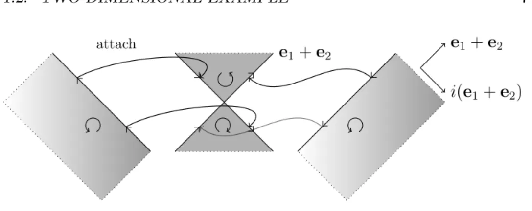
Extending the PS domain: Before deforming the PS domain, the boundary problem has to be dealt with first. The idea is to attach half- planes to the boundary lines spanned by e
1± e
2as illustrated in figure 1.4.
Here it is again crucial that the upper and lower cone have opposite ori-
entations to allow the attachment of the halfplanes in a consistent way. A
parametrisation of the halfplanes is given by
e
1+ e
2e
1+ e
2i(e
1+ e
2)
attach
Figure 1.4: Attaching halfplanes that do not contribute to the integral.
hp
±: R
+× R → C
2(h, x) 7→ ±xe
±− ihe
±,
where e
±= e
1± e
2. A good motivation for this special choice is that dq
1∧ dq
2(e
±, ie
±) = idq
1∧ dq
2(e
±, e
±) = 0
and hence the halfplanes do not contribute to the integral. This is not yet a completely rigorous argument since existence and convergence of the integral still needs to be discussed. The extension of PS is defined as eP S :=
P S + hp
++ hp
−, which is to be understood as a sum of integration chains.
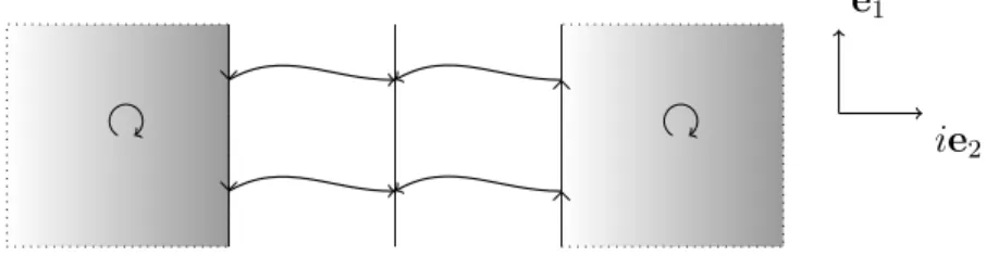
Equivalence of PS and Euclid: The deformation is given by DP S : [0, 1] × [−1, 1] × R → R
2(t, h, x) 7→ x(e
1+ (1 − t)he
2) , Dhp
±: [0, 1] × R
+× R → C
2(t, h, x) 7→ ±x[e
1± (1 − t)e
2] − ih[(1 − t)e
1± e
2] ,
which defines then DeP S = DP S + Dhp
++ Dhp
−. For t = 1 the deformed PS surface degenerates into a line and both halfplanes hp
±are projected into the plane spanned by e
1and ie
2as shown in figure 1.5. Note that Dhp
±(t = 1) : (h, x) 7→ ±xe
1∓ ihe
2. Thus we have DeP S(t = 1) = Euclid.
Now, we want to apply Stokes’ theorem. We use ∂DeP S
= Euclid − DeP S(), where DeP S
:= DeP S|
t∈[,1]. The idea is to deform Euclid, as far as convergence of the integral allows, into P S:
Z
DeP S()
g(~ q, ~a)dq = − Z
DeP S
g(~ q, ~a)d(dq) + Z
Euclid
g(~ q, ~a)dq
= Z
Euclid
g(~ q, ~a)dq . (1.9)
e
1ie
2Figure 1.5: Deformation of PS to Euclid. The two halfplanes are the (de- formed) attached surfaces and the cones are deformed into the vertical line.
Next we have to discuss the limit → 0 carefully.
First consider the P S part. Here, we may apply Fubini’s theorem and perform the x integration first, since for > 0 the integral is exponentially convergent. We define
I
P S(, h) :=
r π
1 − h
2(1 − )
2e
−(a1−a2h(1−))2 1−h2(1−)2
. Then we obtain
lim
→0Z
DP S()
g(~ q, ~a)dq = lim
→0
Z
1−1
dh I
P S(, h) .
The limit lim
→0I
P S(, h) is uniform, since (a
1− a
2h(1 − ))
2> 0 for 1 ≥ ≥ 0 and a
1> a
2≥ 0. Thus the h integral and lim
→0commute.
In particular, this is also true if we replace I
P S(, h) by I ˜
P S(, h) :=
r π
1 − h
2(1 − )
2e
−(a1−a2h)2 1−h2(1−)2
. Then we have the following series of equalities:
→0
lim Z
DP S()
g(~ q, ~a)dq = Z
1−1
dh lim
→0
I
P S(, h)
= lim
→0
Z
1−1
dh I ˜
P S(, h)
= lim
0→0
Z
P S
g(~ q, ~a)χ
0(q)dq ,
where we shift the dependence of the domain of integration to the inte- grand by introducing a regulating function χ
0(q) = exp(−
0q
22). To be more precise, we identify
0= 2 −
2.
It remains to show that the contribution from the hp
±parts vanish. This is done using similar arguments as above. Consider
lim
→0Z
Dhp±()
g(~ q, ~a)dq = lim
→0
Z
∞ 0dh I
hp±(, h) ,
where we define I
hp±(, h) :=
r π
1 − (1 − )
2e
−(±a1−(1−)a2)2
1−(1−)2
e
−2h((1−)a1∓a2)e
−h2(2−2). The last two factors ensure exponential convergence in h. Hence the integral exists and
→0
lim I
hp±(, h) = 0 holds uniformly in h. Thus we can conclude that
→0
lim Z
Dhp±()
g(~ q, ~a)dq = 0 . The proof is finished, since we now have
→0
lim Z
DeP S()
g(~ q, ~a)dq = lim
→0
Z
P S
g(~ q, ~a)χ (q)dq . (1.10)
1.3 General setting and theorem
In this section we present our results in a rather general form. First, we describe the setting and then we state our theorem. Let us note in advance that appendix A contains a systematic discussion of the structures that are used to formulate the theorem and its proof.
All constructions take place in gl(n, C), the space of all complex n × n matrices. The following results also apply to the case where gl(n, C ) is replaced by a complex Lie subalgebra of gl(n, C ). Let s ∈ gl(n, C ) be hermitian with the property s
2= 1. s leads to two involutions
2θ(X) = sXs
−1and γ (X) = −sX
†s
−1on gl(n, C ). In addition we assume that we are given some involutions τ
ion gl(n, C ), which commute with each other and with θ and γ . Then we can define a subspace Q of gl(n, C) as
Q = {Q ∈ gl(n, C )|Q = −γ(Q) and ∀i : Q = σ
iτ
i(Q)} , (1.11) where σ
i∈ {±1} and the τ
ihave to be such that s ∈ Q. The Lie algebra of the relevant symmetry group of Q is given by
3g = {X ∈ gl(n, C)|X = γ(X) and ∀i : X = τ
i(X)} . (1.12) The decomposition of Q into the plus and minus one eigenspaces of θ gives a decomposition into the hermitian and antihermitian parts denoted by Q
+and Q
−. Similarly θ gives the decomposition g = k ⊕ p, where k is the plus
2
In this context involution means an involutive automorphism of Lie algebra.
3
See also section A.1.2 in appendix A.
one eigenspace and p the minus one eigenspace. The commutation relations of these spaces are
4[k, k] ⊂ k , [k, p] ⊂ p , [p, p] ⊂ k , [Q
+, Q
−] ⊂ p ,
[Q
±, Q
±] ⊂ k , [k, Q
±] ⊂ Q
±, [p, Q
±] ⊂ Q
∓. (1.13) Then the parametrisation of the Pruisken-Sch¨ afer domain is given by
P S : p ⊕ Q
+→ Q
(Y, X ) 7→ e
YXe
−Y. (1.14) The parametrisation of the Euclidean domain is given by
Euclid : Q
−⊕ Q
+→ Q
C(Y, X ) 7→ X + iY ,
where Q
C= Q ⊕ iQ. The parametrisation of the Sch¨ afer-Wegner domain is given by
SW : p ⊕ Q
+→ Q
C(1.15)
(Y, X) 7→ X − ibe
Yse
−Y, (1.16) where b is a positive real number. The orientation for P S, Euclid and SW is provided by choosing an orientation of the domain of definition. This induces an orientation on the corresponding domain of integration.
Theorem 1.2. If in the setting above g is the direct sum
5of a semisimple and an Abelian Lie algebra and A ∈ Q with As > 0, then
→0
lim Z
P S
e
−Tr(Q2)−2iTr(QA)χ (Q)dQ = c e
−Tr(A2)(1.17) holds. Here, χ (Q) = exp(
4Tr(Q − θQ)
2) is a regulating function and dQ denotes a constant volume form on Q. c ∈ C \ {0} is a constant that does not depend on A.
The result will be proved by showing that the PS domain can first be extended and then deformed into a standard Euclidean integration domain without changing the value of the integral. Therefore we view DQ as holo- morphic dimQ form on Q
C. In addition it will be shown that the SW domain can also be deformed into this Euclidean integral. Hence the PS and SW domains are contour deformations of the same simple Euclidean Gaussian domain.
The following corollary is the analogue of corollary 1 in [12]:
4
See section A.1.3 in appendix A.
5
This means in particular that the semisimple and the Abelian part commute with
each other.
Corollary 1.1. Let k ⊕Q
+be the direct sum of a semisimple and an Abelian Lie algebra and let h be a maximal Abelian subalgebra of Q
+. Furthermore let g be semisimple and define G = exp(p) exp(k)
6. Then
→0
lim Z
h
Z
G
e
−2iTr(gλg−1A)χ
(gλg
−1)|dg|
e
−Trλ2J
0(λ)|dλ| = ˜ c e
−Tr(A2), holds, where
J
0(λ) = Y
α∈Σ+(p⊕Q−,h)
α(λ)
dαY
α∈Σ+(k⊕Q+,h)
|α(λ)
dα| .
Σ
+(V, h) denotes the sets of positive weights with respect to the adjoint action of h with weight spaces in V .
7d
αare the dimensions of the weight spaces.
|dg| denotes Haar measure on G and |dλ| denotes Lebesgue measure on the vector space h. ˜ c ∈ C \ {0} is a constant that does not depend on A.
The following corollary is the analogue of theorem 1 in [12]:
Corollary 1.2. If the parametrisation P S is nearly everywhere injective and regular, then
lim
→0Z
ImP S
e
−Tr(Q2)−2iTr(QA)χ (Q) sgn(J
0(λ)) |dQ| = ˜ c
0e
−Tr(A2)holds. ImP S denotes the image of P S and the mapping from ImP S to h sending Q to λ is well defined up to a set of measure zero. |dQ| denotes Lebesgue measure on Q. ˜ c
0∈ C \ {0} is a constant that does not depend on A.
1.4 Proof of the theorem
For simplicity we restrict ourselves to the case where g is semisimple. The extension to the more general case is straightforward. The proof is divided into three parts. The first part, 1.4.1, contains the derivation of a new parametrisation of the PS domain, which makes its boundary visible in the domain of definition. Decomposing this parametrisation suitably as a sum of integration cells one obtains an adequate description of the boundary of the PS domain. The second part of the proof, 1.4.2, deals with the extension of the PS domain to a domain ePS without boundary. First we identify good directions into which the PS domain can be extended. Then an extension of PS that does not change the value of the integral is given. Finally in section 1.4.3 we construct a deformation DeP S of the extended PS domain to the Euclidean domain. The deformation satisfies ∂DeP S = Euclid−eP S.
6G
is the unique analytic subgroup of
GL(n,C) with Lie algebra
g.7
See also section A.1.4 in appendix A.
Essentially we want to make rigorous the following schematic application of Stokes:
Z
P S
g(Q, A)dQ = Z
eP S
g(Q, A)dQ
= − Z
DeP S
d(g(Q, A)dQ)
| {z }
=0
+ Z
Euclid
g(Q, A)dQ ,
where we define g(Q, A) := e
−Tr(Q2)−2iTr(QA). Note that the first term in the second line is identically zero since g(Q, A) is holomorphic in Q. At this point a warning is in order: In this form the upper expressions do not make sense. In order for the integrals over P S, eP S and DeP S to exist we have to include some regularisation. This delicate issue is discussed in detail in the last part of section 1.4.3.
1.4.1 A suitable parametrisation of the PS domain
First, we perform a series of reparametrisations to derive a more convenient parametrisation which allows to use the geometric intuition from the two dimensional example for the PS domain and its boundary. Finally we de- compose the parametrisation into different parts, allowing the application of Stokes’ theorem. In the following we use standard results from Lie theory.
A good reference is [14]. In addition appendix A gives a detailed description of the constructions we use.
Reparametrisation I: Decomposition of p
The goal of the next three reparametrisations is to evaluate P S(Y, X) = Ad(e
Y)X in more detail. Key to this is choosing a maximal Abelian sub- algebra a in p, whose adjoint action on Q = Q
+⊕ Q
−can be diagonalised simultaneously.
8To begin with, we decompose the parameter space p to see the algebra a. Therefore we define the compact group K := exp(k) and the centraliser Z
K(a) of a in K . Furthermore a
o+⊂ a denotes the interior of a fixed Weyl chamber.
9Consider the mapping
R
I: a
o+× K/Z
K(a) → p
(H, [k]) 7→ kHk
−1.
R
Iis obviously well defined. In appendix A.2.1 it is shown that R
Iis injective and regular. Hence R
Iis a diffeomorphism onto. Note, that p \ Im(R
I) is a set of measure zero since p = ∪
k∈Kkak
−1 10and Im(R
I) =
∪
k∈Kk(a \ ∪
αker α)k
−1where α are the restricted roots with respect to a.
118
See section A.1.4 in appendix A.
9
See [14] for a definition and properties of Weyl chambers.
10
This standard result, which can be found in [14], is used without further explanation.
11
See section A.1.4 in appendix A.
To be precise we want to use the parametrisation P S ◦ R
I: a
+× K/Z
K(a) × Q
+→ Q
(H, [k], X) 7→ e
kHk−1Xe
−kHk−1.
The orientation of P S is given by an orientation of p ⊕ Q
+. Declaring R
Ito be orientation preserving induces an orientation on a
o+× K/Z
K(a) × Q
+. To keep the notation simple we call each new parametrisation again P S.
Reparametrisation II: Twisting K/Z
K(a) and Q
+In this section we prepare further evaluation of the a action in the next subsection. Consider the reparametrisation
R
II: K ×
ZK(a)Q
+→ K/Z
K(a) × Q
+[kz
−1, zXz
−1] 7→ ([k], kXk
−1) .
Note that z ∈ Z
K(a) in the expression [kz
−1, zXz
−1] indicates group actions of Z
K(a) on K and on Q
+. These group actions are used to define the bundle K ×
ZK(a)Q
+. The inverse of R
IIis given by
R
−1II: K/Z
K(a) × Q
+→ K ×
ZK(a)Q
+([k], X) 7→ [k, k
−1Xk] .
R
IIis obviously a diffeomorphism and therefore can be used as a reparametri- sation to obtain
P S ◦ R
II: a
o+× K ×
ZK(a)Q
+→ Q
(H, [kz, z
−1Xz]) 7→ e
kHk−1kXk
−1e
−kHk−1= ke
HXe
−Hk
−1as new parametrisation.
Reparametrisation III: Decomposition of Q
+The weight decomposition of Q with respect to the adjoint action of a is given by
Q = Q
0⊕ M
α∈Σ+(Q,a)
(Q
α⊕ Q
−α) .
Here Σ
+(Q, a) denotes the set of posive weights. Defining
Q
+,α:= Fix
θ(Q
α⊕ Q
−α) and Q
+,0= Fix
θ(Q
0) ,
we obtain the decomposition
Q
+= Q
+,0⊕ M
α∈Σ+(Q,a)
Q
+,α.
For more details and properties of this decomposition see appendix A.1.4.
Since Z
K(a) is a subset of K, and, by definition, commutes with the ad(a) action on Q, the decomposition is compatible with the bundle structure of K ×
ZK(a)
Q
+. Again, the reparametrisation R
III: a
+× K ×
ZK(a)
Q
+,0⊕ M
α∈Σ+(Q,a)
Q
+,α→ a
+× K ×
ZK(a)
Q
+(H, [kz, z
−1M z, z
−1X
αz]) 7→
H, h
kz, z
−1M + X
α∈Σ+(Q,a)
X
αz i
,
is an orientation preserving diffeomorphism.
We define a mapping φ : Q
+→ Q
−implicitly through
[H, X
α] = α(H)φ(X
α) and [H, φ(X
α)] = α(H)X
α(1.18) for all H ∈ a. See also appendix A.1.3. Using (1.18) a short calculation gives
e
ad(H)X
α= cosh(α(H))X
α+ sinh(α(H))φ(X
α) . Moreover, the parametrisation can be rewritten to
P S ◦ R
III: a
+× K ×
ZK(a)Q
+,0⊕ M
α∈Σ+(Q,a)
Q
+,α→ Q
(H, [k, M,X
α]) 7→ Ad(k) h
M + X
α∈Σ+(Q,a)
cosh(α(H))X
α+ sinh(α(H))φ(X
α) i .
In the following P S ◦ R
IIIis denoted simply by P S.
Reparametrisation IV: Transfer boundary to a
+As a motivation for the next reparametrisation of Q
+,αone might imag-
ine the coordinate line belonging to λH ∈ a
+as a hyperbola. We want
to have a simple Euclidean picture of the situation. Thus we change our
parametrisation in a way that these coordinate lines are straight lines, see
figure 1.6. Most importantly such a reparametrisation simplifies the view
on the boundary of the PS domain, as is discussed in the next subsection.
Q
+,αQ
−,αQ
+,αQ
−,αFigure 1.6: Motivation for the third reparametrisation step. The dashed lines are coordinate lines of λH ∈ a
+.
Thus, the fourth reparametrisation we use is given by R
IV: a
+× K×
ZK(a)
Q
+,0⊕ M
α∈Σ+(Q,a)
Q
+,α→ a
+× K ×
ZK(a)
Q
+,0⊕ X
α∈Σ+(Q,a)
Q
+,α(H, [k, M, X
α]) 7→
H, h
k, M, 1
cosh(α(H)) X
αi ,
which is also an orientation preserving diffeomorphism. We obtain P S ◦ R
IV: a
+× K ×
ZK(a)Q
+,0⊕ M
α∈Σ+(Q,a)
Q
+,α→ Q
(H,[k, M, X
α]) 7→ Ad(k) h
M + X
α∈Σ+(Q,a)
X
α+ tanh(α(H))φ(X
α) i , (1.19) which we again call P S in the following.
Boundary of the PS domain
In this subsection we explain why parametrisation (1.19) is useful to get an intuition for the geometry and especially the boundary of the PS domain.
This discussion is not meant to be rigorous but motivates the next steps of the proof.
The geometry can be described using Tr(XY
†) as an Ad(K)-invariant
scalar product on Q. Thus for the moment we forget about the Ad(K)
Q
+,αQ
−αFigure 1.7: Interior of the PS domain. The rest is generated by the K action.
action and restrict ourselves to the inner part iP S : a
+×
Q
+,0⊕ M
α∈Σ+(Q,a)
Q
+,α→ Q
(H, M, X
α) 7→ M + X
α∈Σ+(Q,a)
X
α+ tanh(α(H))φ(X
α) .
Note that the different Q
+,αand also Q
−,αare all orthogonal to each other.
Hence we consider only one α ∈ Σ
+(Q, a) at a time:
X
α+ tanh(α(H))φ(X
α) ,
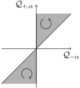
for which figure 1.7 is a good two dimensional picture. Except for the additional presence of the Weyl group, figure 1.7 is in agreement with figure 1.3 of the two dimensional example.
It is clear that the boundary is reached when some α(H) goes to ±∞ and hence tanh goes to ±1. To put it differently, the boundary of the domain of integration can be reached through a limit in the parameter space a
+. Note that acting with K on the boundary, identified in the inner part of the P S parametrisation, the full boundary is generated.
Since we want to get rid of the boundary by attaching halfplanes to the PS domain, we want to give a parametrisation which reaches all boundary points. This implies performing the limit explicitly and thus making the boundary visible in the domain of definition.
Decomposition of the parametrisation P S
The problem we face is to perform the limit in a
+in a well defined way.
Therefore we have to discuss the weights α ∈ Σ
+(Q, a) in more detail.
First note that α(H) might change sign on a
+since a
+is defined with
respect to the restricted roots β ∈ Σ(g, a). Within this subsection α will
always denote a weight in Σ
+(Q, a).
The main idea is to decompose the P S parametrisation by decomposing a
+into different cones on which sgn(α(H)) stays constant or α(H) goes to zero for all α ∈ Σ
+(Q, a).
The closures of the connected components of a
+\ ∪
αker(α) are pointed polyhedral cones, whose edges lie in the intersections of hyperplanes defined by the kernels of the weights in Σ
+(Q, a). Let us consider one of these pointed cones. It can also be defined as an intersection of halfspaces or as non-negative linear combination of some generators H
i∈ a. The generators are the edges of the cone. In general the number of generators might be greater than n := dim a. But each pointed cone can be triangulated (without introducing new vertices) into simplicial cones, i.e., cones where the number of generators equals dim a. See for example [13]. Now we fix triangulations for each original pointed polyhedral cone. Thus we obtain a decomposition of a
+into simplicial cones, which we denote by a
+,cand
a
+= [
c∈C
a
+,c, (1.20)
where C is an index set for the different cones. Denote the generators/edges of a
+,cby H
i,c. Then we can represent H ∈ a
+,cuniquely as
H =
n
X
i=1
h
iH
i,c(1.21)
with coefficients h
i∈ R
+. The important thing is that the sign of all α on a given simplicial cone stays constant. However it is still allowed that α vanishes at the boundary of the simplicial cone. Thus we decompose our parametrisation as follows:
P S = X
c∈C
P S|
a+,c×K×ZK(a)(Q+,0⊕L
α∈Σ+(Q,a)Q+,α)
.
In the following we hide the index c of H
i,cand use the notation H = P
i
h
iH
ifor H ∈ a
+which implies the choice of H
ias described above. By construction we then have h
i≥ 0.
Reparametrisation V: Making the boundary visible
To make the boundary visible in the domain of definition we define a
B,c=
(
n≡dimaX
i=1
h
iH
i∈ a
+,c|∀i : 0 ≤ h
i≤ 1 )
. and use the reparametrisation
R
V,c: a
oB,c→ a
+,cn
X
i=1
h
iH
i7→
n
X
i=1
h
i1 − h
iH
i,
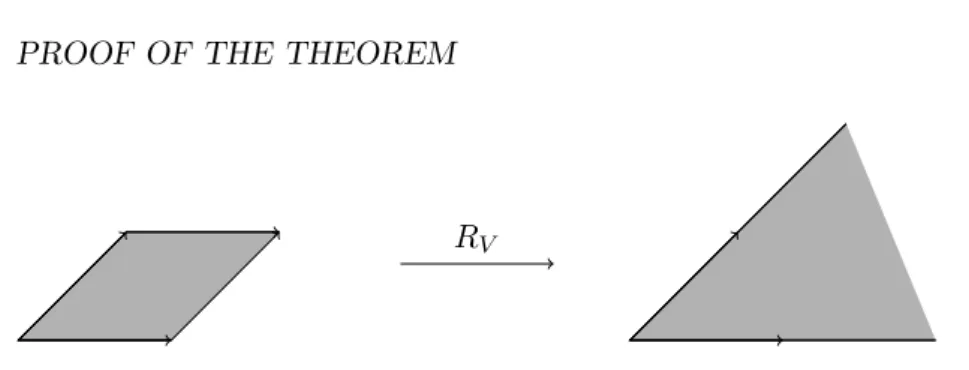
which is an (orientation preserving) diffeomorphism onto for each simplicial cone. The reparametrisation is visualised in figure 1.8. Note that there is an obvious diffeomorphism between [0, 1]
nand a
B,c. Defining for each cone c ∈ C
P S
c: [0, 1]
n× K ×
ZK(a)
Q
+,0⊕ M
α∈Σ+(Q,a)
Q
+,α→ Q
(h
i,[k, M, X
α]) 7→
Ad(k) h
M + X
α∈Σ+(Q,a)
X
α+ tanh X
i
h
i1 − h
iα(H
i)
φ(X
α) i
, (1.22) we have P S = P
c∈C
P S
cas an equation of integration chains. It is impor- tant to keep in mind that [0, 1]
nis essentially a
B,c, which can be seen as a truncated cone in a
+.
In the following we want to give the notion ‘boundary of the PS domain’
a precise meaning. For integration cells, i.e., differentiable mappings defined on a cube, the boundary operator ∂ is defined as usual. ∂ can also be applied to integration chains, i.e. formal linear combinations of cells. In principle we would have to decompose each P S
cinto cells to apply ∂. In the following we argue that we can treat each P S
ceffectively as cell with the boundary operator ∂ acting just on the [0, 1]
npart of the domain of definition.
First we have to show that P S
ccan be extended to a neighbourhood of [0, 1] on which it is still differentiable. This property is included in the definition of an integration cell. It is needed to define the orientation of the boundary. Let us first concentrate on the tanh term in the P S
cparametri- sation. Since
lim
hj→1
∂
hjtanh h X
ni=1
h
i1 − h
iα(H
i) i
= 0 , (1.23)
generalises to all higher (and mixed) partial derivatives, we extend P S
cfor h
i> 1 by setting it constant in that direction. To be more precise we define for h
i> 0
P S
c(. . . , h
i, . . . ) := P S
c(. . . , 1, . . . ) .
For h
i< 0 just analytically continue the parametrisation P S
c. Using (1.23) it can be easily shown that the extension of P S
cto a neighbourhood of [0, 1]
nis differentiable.
Now we present an argument that we can treat each P S
ceffectively as cell and that it is enough to let the boundary operator ∂ act on the [0, 1]
npart of the domain of definition. Since K is a closed compact manifold it suffices to discuss boundary contributions arising from a decomposition of Q
+,0⊕ P
α∈Σ+(Q,a)
Q
+,αinto cells. Inspecting our parametrisation we see
R
VFigure 1.8: su(2, 2) example for R
Vmapping a
Bon the left hand side to a
+on the right side. In this example there is only one simplicial cone, i.e.
|C| = 1.
that going to infinity in the domain of definition implies going to infinity in the domain of integration. In section 1.4.3 we show that the integrand converges exponentially on this domain and hence all possible boundary contributions vanish.
Only the part [0, 1]
n, or equivalently, the part a
B,cof the domain of definition, leads to a nontrivial boundary. The boundary parts coinciding with boundaries of a
+are of codimension at least two, and thus do not contribute. For a detailed argument concerning this point see appendix A.2.3.
1.4.2 Extending the PS domain
In this section we construct an extension of the PS domain that has no relevant boundary. This means we have to attach additional domains to the boundary of the PS domain. The idea is to attach a halfline to each boundary point. The direction of this halfline should be a convergent one, and it should also guarantee that the attached domain does not contribute to the integral when integrated against f (Q) dQ. First we determine such a direction, and then give a parametrisation of the attached domains. In the following it is often convenient to view B(X, Y ) := Tr(XY ) as a bilinear form on Q
C.
Good directions
We want to extend the PS domain from the boundary into an imaginary null directions E
i. The terminology ‘null direction’ conveys two things. First E
iis a null direction in the sense that B(E
i, E
i) = 0. And second the extension in this direction does not contribute to the integral since the volume form vanishes for these directions. E
ishall also be a convergent direction. It is reasonable to expect that the term exp(−2iB(Q, A)) guarantees convergence in this situation if
< [iB(Ad(k)E
i, A)] = <[i Tr(s
−1Ad(k)E
iAs)] > 0 . (1.24)
In order for (1.24) to hold it suffices that isAd(k)E
i≥ 0 and E
i6= 0, since As > 0 by assumption. For our definition of E
ibelow it is important that for Y ∈ p
s
−1e
Yse
−Y= e
−2Y> 0 holds. The natural choice for E
iis
E
i:= −2i lim
t→∞
Ad(e
tHi)s
max
α∈Σ+(Q,a)e
|α(tHi)|. (1.25) Note that Z
K(a) acts trivially on E
i. Let us also mention again that we have hidden the dependence of H
ion c ∈ C. Thus E
ialso depends on c ∈ C.
It is instructive to give a more explicit form of E
i. Since s ∈ Q
+we have the decomposition
s = M
s+ X
α∈Σ+(Q,a)
X
s,α, (1.26)
where M
s∈ Q
+,0and X
s,α∈ Q
+,α. A short calculation gives Ad(e
H)s = M
s+ X
α∈Σ+(Q,a)
cosh(α(H))X
s,α+ sinh(α(H))φ(X
s,α) .
This shows that the limit in (1.25) exists. In addition E
i6= 0 because a → Q
−, H 7→ [H, s] is injective. The properties of this mapping are discussed in detail in appendix A.1.3. Note also that E
idepends on the chosen simplicial cone c, and that B (E
i, E
i) = 0. Most importantly inequality (1.24) holds (even without taking the real part).
is
−1E
ican be regarded as an orthogonal projection on the weight space (in the vector space on to which g acts) with the largest eigenvalue with respect to the e
Hiaction.
Parametrisation of the extension
In this section we suggest an extension of the PS domain and then check that it has all the desired properties. The extended PS domain (ePS) is parametrised by
eP S : a
+×K ×
ZK(a)Q
+,0⊕ X
α∈Σ+(Q,a)
Q
+,α→ Q
C(H, [k,M, X
α]) 7→
Ad(k) h
M + X
α∈Σ+(Q,a)
h
X
α+ tanh X
j
ξ(h
j)α(H
j)
φ(X
α) i
+
n
X
j=1
Θ(h
j− 1)(h
j− 1)E
ji
,
where we use
ξ(h) :=
h1−h
h < 1
∞ h ≥ 1
Θ is the step function. The attached surface starts as soon as some h
i> 1.
The limit contained in the expression tanh( P
j
ξ(h
j)α(H
j)) is well de- fined because sgn(α(H
j)) is the same for all i with α(H
i) 6= 0. Note that the mapping eP S is well defined since Z
K(a) acts trivially on the E
i.
In the following we decompose the parametrisation eP S into different pieces, which can be treated as integration cells. Remember that we al- ready have the corresponding decomposition P S = P
c∈C
P S
c. For eP S the situation is slightly more involved as we have to account explicitly for the limit being taken, i.e., which h
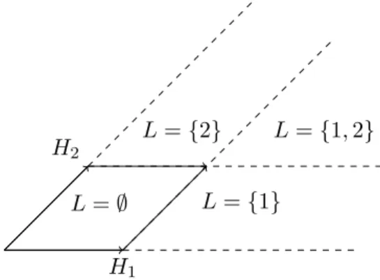
iare larger than one. The different possibil- ities are characterised by subsets L ⊂ {1, 2, . . . , n = dim a}. The extended parametrisation decomposes into several pieces eP S
L,c. The situation is visualised in figure 1.9. To be able to write down eP S
L,cexplicitly we define
Σ
L,6=:= {α ∈ Σ
+(Q, a)|∃i ∈ L : α(H
i) 6= 0}
and
Σ
L,=:= {α ∈ Σ
+(Q, a)|∀i ∈ L : α(H
i) = 0} . Then we have for each L ⊂ {1, 2, . . . , n = dima} and c ∈ C
eP S
L,c: [0, 1]
n−|L|× [1, ∞)
|L|× K ×
ZK(a)Q
+,0⊕ X
α∈Σ+(Q,a)
Q
+,α→ Q
C(h
i, [k,M, X
α]) 7→
Ad(k) h
M + X
α∈ΣL,6=
(X
α+ sgn(α(H
i))φ(X
α))
+ X
α∈ΣL,=
h
X
α+ tanh X
nj=1
ξ(h
j)α(H
j)
φ(X
α) i
+ X
j∈L
(h
j− 1)E
ji .
Next we present an argument that eP S
L,ccan be treated as an integration cell and that the boundary operator ∂ only acts on [0, 1]
n−|L|× [1, ∞)
|L|. First we discuss the extension of eP S
L,cto a neighbourhood of [0, 1]
n−|L|× [1, ∞)
|L|. For i / ∈ L and h
i> 0 we define
eP S
L,c(. . . , h
i, . . . ) := eP S
L,c(. . . , 1, . . . ) ,
and for h
i< 0 or i ∈ L and h
i< 1 we analytically continue the parametrisa-
tion eP S
L,c. The boundary operator ∂ applied to eP S
L,cis evaluated using
H
1H
2L = ∅
L = {2}
L = {1}
L = {1, 2}
Figure 1.9: This figure shows a
+for g = su(2, 2). a
+is decomposed into the domains of definition for the different mappings eP S
L,cin a
+with L ⊂ {1, 2}.
exactly the same reasoning as for the P S
cmappings. Thus ∂ acts only on [0, 1]
n−|L|× [1, ∞)
|L|. To see that
∂eP S = X
c∈C
X
L⊂{1,2,...,n}