The chronology of Late Glacial and Holocene dune development in the northern Central European lowland reconstructed by optically stimulated luminescence (OSL) dating

The chronology of Late Glacial and Holocene dune development in the northern Central European lowland reconstructed

by optically stimulated luminescence (OSL) dating

I n a u g u r a l – D i s s e r t a t i o n

zur

Erlangung des Doktorgrades

der Mathematisch-Naturwissenschaftlichen Fakultät der Universität zu Köln

vorgelegt von

Alexandra Hilgers

aus Neuss

Köln, 2007

Berichterstatter : Prof. Dr. U. Radtke Prof. Dr. G. Schellmann PD Dr. R. Zeese

Tag der mündlichen Prüfung: 6. November 2006

Contents

1. Introduction... 15

2. Aims of the study ... 16

3. Luminescence dating of sediments... 19

3.1 Basic principle, history and current trends of luminescence dating... 19

3.2 Source and nature of ionising radiation in sediments ... 25

3.2.1 Types of radiation and their characteristics... 26

3.2.2 Radionuclides in sediments as radiation source... 28

3.3 Dose rate determination ... 31

3.3.1 Conversion of energy emission into dose rates for quartz as absorbing matter... 31

3.3.2 Methods for dose rate determination... 33

3.3.2.1 Neutron activation analysis (NAA) ... 33

3.3.2.2 High-resolution gamma-ray spectrometry ... 34

3.3.2.3 In-situ gamma-dose measurements... 36

3.3.3 Dose rate variation and sources of error ... 36

3.3.3.1 Radioactive disequilibria ... 37

3.3.3.2 Variation in the radiation field by inhomogeneities... 40

3.3.3.3 Influence of uncertainty in water content variations... 41

3.3.3.4 Internal dose rate... 43

3.3.3.5 Variation of the cosmic ray dose contribution... 43

3.3.4 Results of dose rate (D

) determination ... 46

3.3.4.1 Results of neutron activation analysis (NAA) ... 46

3.3.4.2 Comparison of NAA and gamma-spectrometry results... 48

3.3.4.3 In-situ gamma-dose measurements... 51

3.3.4.4 Evidence for disequilibrium and its implication for age calculation ... 53

3.3.4.5 Assessment of the internal dose rate in quartz... 57

3.3.4.6 Water content estimation ... 58

3.3.4.7 Impact of varying overburden thickness on the cosmic dose contribution ... 61

3.3.5 Dose rate calculation... 64

3.4 Using quartz as ‘natural dosimeter’ for palaeodose

estimation by OSL... 65

3.4.1 Physical background for luminescence phenomena ... 65

3.4.1.1 Crystal structure, defects, centres and traps... 66

3.4.1.2 The luminescence phenomenon - a simple ‘one-trap/one-centre’ model ... 71

3.4.2 Luminescence properties of quartz ... 73

3.4.2.1 Characteristics of electron traps and TL peaks of quartz... 73

3.4.2.1.1 Thermal stability ... 76

3.4.2.1.2 Number of traps... 79

3.4.2.1.3 Bleachability ... 81

3.4.2.2 Characteristics of luminescence centres and emissions of quartz... 83

3.4.2.2.1 The 360-440 nm (near-UV-violet) emission band... 86

3.4.2.2.2 The 460-500 nm (blue) emission ... 87

3.4.2.2.3 The 600-650 nm (orange) emission... 87

3.4.3 Extraction of the suitable OSL dating signal of quartz... 88

3.4.3.1 Appropriate preheat procedures ... 90

3.4.3.2 Appropriate optical stimulation and signal detection ... 97

3.5 Equivalent dose determination on sand-sized quartz grains... 101

3.5.1 Sample preparation for equivalent dose measurements ... 101

3.5.1.1 Impact of feldspar contamination ... 102

3.5.2 The single-aliquot regenerative-dose (SAR) protocol for coarse- grain quartz ... 104

3.5.2.1 The routine SAR measurement procedure ... 105

3.5.2.2 Basic principle of sensitivity correction in the SAR procedure... 107

3.5.2.3 Testing the robustness of the SAR protocol ... 110

3.5.2.3.1 Influence of test dose size ... 110

3.5.2.3.2 Influence of the pre-heat temperature and thermal transfer effects... 112

3.5.2.3.3 Influence of irradiation strength and the measurement equipment ... 119

3.6 Results of the equivalent dose (D

) determination... 122

3.6.1 Calculation procedure for equivalent dose estimates ... 122

3.6.1.1 Determination of the sensitivity corrected OSL signal... 122

3.6.1.2 Determination of the equivalent dose (D

)... 126

3.6.1.3 Testing for normal distribution and impact of outlier exclusion ... 130

3.6.1.4 Discussion of the quality of the equivalent dose estimates... 134

3.6.2 ‘Aeolian deposits are usually well-bleached’ – a critical discussion ... 137

3.6.2.1 Inconsistency with the chronostratigraphy ... 138

3.6.2.2 Detecting poor bleaching by OSL signal analysis ... 139

3.6.2.2.1 The D

versus illumination time plot... 139

3.6.2.2.2 Correlation of OSL intensity versus equivalent dose ... 140

3.6.2.3 Identification of poor bleaching in D

distributions... 143

3.6.2.3.1 Asymmetry of D

distributions... 143

3.6.2.3.2 Thresholds for the relative scatter in equivalent dose distributions... 146

3.6.2.3.3 Determination of the natural variation in D

estimates from well-bleached deposits ... 148

3.6.3 The natural variation in equivalent dose estimates in the dose range 0-20 Gy from well-bleached aeolian deposits ... 149

3.6.3.1 Measurement conditions ... 149

3.6.3.2 Photon counting statistics ... 150

3.6.3.3 Dose range ... 151

3.6.3.4 Intrinsic luminescence properties ... 151

3.6.3.5 Incomplete zeroing of the luminescence signal ... 153

3.6.3.6 Post-depositional sediment mixing ... 157

3.6.3.7 Heterogeneity in natural dosimetry... 161

3.6.3.8 Determination of the threshold υ-value for natural samples... 162

3.6.4 Equivalent dose calculation... 164

3.7 Age calculation and plausibility testing ... 165

4. The study sites ...168

4.1 The position of the study area... 168

4.1.1 The European Sand Belt ... 168

4.1.2 Characterisics of the dunefields in the study area ... 170

4.1.3 Chronology of the Weichselian glaciation ... 172

4.1.4 OSL sampling strategy ... 175

4.2 The 'Finow soil' - a palaeosol as stratigraphic marker horizon... 176

4.3 Site descriptions and dating results... 177

4.3.1 Dune sites in the Elbe 'urstromtal' ... 178

4.3.1.1 Site ‘Neuhaus’ (N) ... 180

4.3.1.2 Site 'Schletau' (STA)... 183

4.3.2 Dune sites in the Głogów -Baruth 'urstromtal' ... 186

4.3.2.1 Site 'Glashütte' (G) ... 186

4.3.2.2 Site 'Cottbus' (C) ... 191

4.3.2.3 Site 'Jänschwalde' (J) ... 196

4.3.2.4 Sites 'Jasień' (JA, JB, JC) ... 198

4.3.3 Dune sites in the Toruń-Eberswalde ‘urstromtal’ and on the Schorfheide sandur ... 207

4.3.3.1 Site 'Finow' - The 'Postdüne' (FA, FB, FC) ... 209

4.3.3.2 Site 'Spechthausen' (S) ... 217

4.3.3.3 Site 'Melchow' (M)... 218

4.3.3.4 Site 'Rosenberg' (R) ... 219

4.3.3.5 Site ‘Schorfheide A’ (SHA)... 221

4.3.3.6 Site ‘Schorfheide B’ (SHB) ... 223

4.3.4 Dune sites in the ‘Ueckermünder Heide’ basin... 226

4.3.4.1 Site 'Ueckermünde-A' (UMA) ... 228

4.3.4.2 Site 'Ueckermünde-D' (UMD) ... 230

4.3.4.3 Site 'Ueckermünde-B' (UMB)... 232

4.3.4.4 Site 'Ueckermünde-C' (UMC)... 233

4.3.5 Dune sites in the Altdarss area ... 236

4.3.5.1 Site 'Altdarss-4' (AD4)... 238

4.3.5.2 Site 'Altdarss-1' (AD1)... 241

5. Discussion of the results ...244

5.1 Comparison with radiocarbon ages ... 244

5.2 Reconstruction of dune development by OSL dating of quartz ... 247

5.2.1 Lateglacial phase of dune formation and reactivation ... 251

5.2.1.1 Relation between dune formation and Lateglacial climate and vegetation changes ... 253

5.2.1.1.1 The onset of aeolian deposition... 258

5.2.1.1.2 The early-Lateglacial period of dune formation ... 261

5.2.1.1.3 The late-Lateglacial period of dune formation and reactivation... 267

5.2.1.2 Influence of human beings on Lateglacial landscapes... 273

5.2.2 Multiple events of dune reactivation in the Holocene ... 274

5.2.2.1 Relevance of Holocene climate oscillations for dune remobilisation... 274

5.2.2.2 Relation between human impact and dune reactivation in the Holocene ... 277

5.2.2.2.1 9 ka peak ... 277

5.2.2.2.2 6.3 ka ... 279

5.2.2.2.3 4.5 ka ... 281

5.2.2.2.4 3.5 ka ... 282

5.2.2.2.5 2.6 ka ... 283

5.2.2.2.6 300 AD ... 285

5.2.2.2.7 Break from 400-900 AD ... 286

5.2.2.2.8 1100 and 1300 AD ... 287

5.2.2.2.9 Break after 1350 AD ... 288

5.2.2.2.10 1600-1800 AD ... 289

5.3 The chronostratigraphy of dune development in the European Sand Belt – New insights? ... 290

5.3.1 Establishment of a chronology of dune construction by luminescence dating... 291

5.3.2 Comparison of the OSL record with existing models of aeolian activity... 295

6. Conclusions...299

7. Summary ...305

8. Zusammenfassung ...311

References... 319

Appendix A: Dose rate data tables

Appendix B: Choice of measurement protocol and mineral fraction for dating Appendix C: Luminescence measurement equipment and beta source

calibration

Appendix D: Equivalent dose determination

Appendix E: Results of OSL dating and list of

C ages

Appendix F: Location of study sites and comparison of analytical results

Danksagung/Acknowledgements

List of tables

Table 1: Natural radioisotopes relevant for luminescence dating. ... 28 Table 2: Dose rates for the U and Th decay chains and K calculated for sand-sized

grains of quartz as absorbing matter. ... 32 Table 3: Beta dose absorption and attenuation factors for spherical, source-free quartz

grains with a diameter of 100 or 200 µm in a uniform matrix containing 12

ppm Th, 3 ppm U, and 0.83 % K. ... 33 Table 4: Dose rates for the U and Th decay chains and K calculated for sand-sized

grains of HF etched quartz grains based on the data summarised in Table 4. ... 48 Table 5: Summary of trap characteristics and procedures for the extraction of main

OSL signal suitable for quartz dating. ... 90 Table 6: The single aliquot regenerative (SAR) dose protocol for quartz after

M URRAY and W INTLE (2000)... 106 Table 7: Results of dose recovery tests for five quartz samples of this study... 136 Table 8: Summary of the υ-values obtained from ‘dose recovery tests’ carried out on

8mm and 1mm aliquots... 152 Table 9: Summary of the equivalent dose measurements using 1mm aliquots for eight

different aeolian samples. ... 155 Table 10: Dating of the Late Weichselian glacial limits in northeast Germany and

northwest Poland... 175 Table 11: The levels of fluvial-glaciofluvial discharge in the ‘Eberswalde’ ice-

marginal valley and their correlation to the different stages of the inland-ice. ... 209 Table 12: Summary of the model on aeolian sand deposition proposed by K ASSE

(2002). ... 297

Table A 1: Radionuclide concentrations of all samples determined either by neutron

activation analyis (NAA) or by gamma-ray spectrometry (γ-spec.)... 1 Table A 2: Results of the duplicate neutron activation analysis. ... 5 Table A 3: Results of in-situ gamma dose rate measurements. ... 6 Table A 4: Summary of parameters for dose rate calculation and finally resulting dose

rates. ... 7

Table B 1: Technical parameters used for comparative luminescence measurements. ... 9

Table D 1: Results of the equivalent dose calculation. ... 1 Table D 2: Comparison of the equivalent dose values and OSL ages obtained for

8mm and 1mm aliquots... 8

Table E 1: List of OSL dating results... 1

Table E 2: Summary of radiocarbon ages and the calibration results... 7

List of figures

Fig. 1: Multi proxy database for palaeclimate reconstruction (MPDB)... 18

Fig. 2: Basic principles of luminescence dating... 20

Fig. 3: Interaction of charged particles with atoms... 26

Fig. 4: Decay chains of uranium-238 and thorium-232. ... 30

Fig. 5: The radioactive decay of potassium-40. ... 30

Fig. 6: Likely causes for disequilibrium in the

U decay chain... 38

Fig. 7: Variations in environmental radiation field. ... 40

Fig. 8: Cosmic dose variation with depth below surface. ... 45

Fig. 9: Comparison of the duplicate neutron activation analysis results... 47

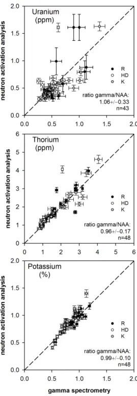
Fig. 10: Comparison of the gamma-ray spectrometry results with those obtained by neutron activation analysis... 50

Fig. 11: Comparison of the in-situ gamma-radiation measurement with the results of neutron activation analysis (NAA) and laboratory high-resolution gamma- spectrometry... 52

Fig. 12: Comparison of

U and

Ra contents from NAA and gamma-ray spectrometry, respectively, to check for radioactive disequilibria in the upper half of the uranium decay chain... 54

Fig. 13: High-resolution low-level gamma-ray spectrometry results for samples from wet environments being suspected of being not in equilibrium state. ... 56

Fig. 14: Distribution of ‘as found’ water contents (expressed as water mass/dry mass) determined for 182 dune sand samples taken from dunes sites within the European Sand Belt... 59

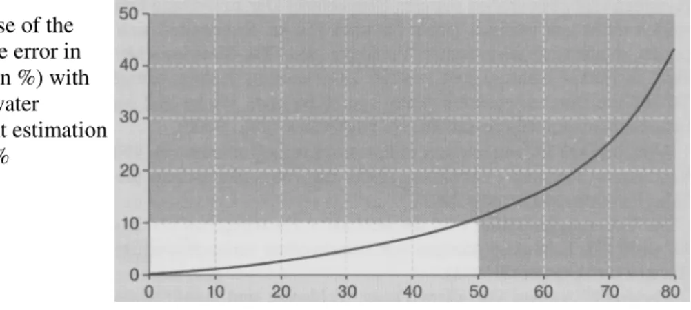
Fig. 15: Impact of erroneous water content assumptions on the relative uncertainty of luminescence ages... 61

Fig. 16: The problem of modelling the cosmic dose contribution at sites with multiple phases of sedimentation. ... 63

Fig. 17: The crystal structure of alpha-quartz. Chemically quartz (SiO

) is quite a simple structure. ... 69

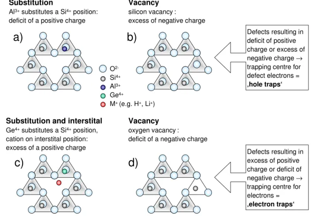
Fig. 18: Some typical defects in the crystal structure of quartz. ... 70

Fig. 19: Energy-level representation of the OSL process. ... 72

Fig. 20: a) TL glow curves obtained for quartz which has been bleached (100 s green light stimulation at 25°C), irradiated (beta dose of 43 Gy) and preheated for

10 s at 110°C... 74 Fig. 21: TL glow curves obtained for six aliquots of sedimentary quartz. ... 76 Fig. 22: Illustration of the correlation of the TL peak temperature, trap depth, and

lifetime. ... 78 Fig. 23: Illustration of the problem of saturation of the electron trap population with

increasing irradiation dose. ... 79 Fig. 24: Changes in sensitivity with repeated luminescence measurements... 81 Fig. 25: Radioluminescence spectra of quartz. ... 84 Fig. 26: a) Correlation of TL peak temperatures and main luminescence emission

bands in quartz (from K RBETSCHEK et al. 1997: 707). b) Energy level diagram including a variety of electron traps (T1-6) and three different recombination sites (R1-3) allowing emission of luminescence in three

different wavelengths... 85 Fig. 27: The OSL emission spectrum of Australian sedimentary quartz measured after

stimulation with 647 nm laser light showing only a single emission band

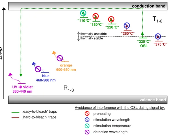
centred on 365 nm... 86 Fig. 28: Simplified energy level scheme illustrating electron traps (T

) and

luminescence centres (R

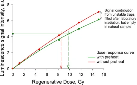
) involved in luminescence processes in quartz. ... 89 Fig. 29: Effect of thermal treatment after laboratory irradiation on the dose response

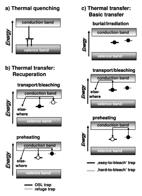
curve... 91 Fig. 30: Effects in the OSL process of quartz induced by thermal treatment of the

sample. ... 93 Fig. 31: Simplified energy band model illustrating the phototransfer effect with the

OSL trap and a competing shallow, light-sensitive trap. ... 96 Fig. 32: Exponential relationship between OSL intensity (In/I) of quartz and photon

energy of the stimulation source. ... 97 Fig. 33: Relation between optical stimulation, OSL emission of quartz and signal

detection. ... 99 Fig. 34: Shine down curves for one aliquot with etched quartz and one with unetched

quartz of the same sample... 103 Fig. 35: Determination of the D

for one aliquot of sample F9 by using the routine

application of the SAR protocol as summarised in Table 6... 107

Fig. 36: High-resolution regenerated growth curve for one aliquot of sample F5... 108

Fig. 37: Relationship between the regeneration net OSL signal (background subtracted) and the subsequent net OSL signal after the test dose to monitor sensitivity changes over repeated measurement cycles (samples F2 and F5,

site ‘Finow’)... 109 Fig. 38: Dependence of D

, reproducibility and recuperation on the variation of the

test dose (relative to D

)... 112 Fig. 39: Dependence of D

, reproducibility and recuperation on the variation of

preheat temperature... 113 Fig. 40: Illustration of preheat protocols... 114 Fig. 41: Influence of preheat temperature and the magnitude of the test dose on

thermal transfer. ... 117 Fig. 42: Equivalent dose determination using irradiation sources of different strength. ... 120 Fig. 43: Individual steps of equivalent dose determination using the single aliquot

regenerative (SAR) protocol for quartz. ... 124 Fig. 44: Comparison of SAR measurements using 3 different regenerative doses or

five different irradiation doses, respectively... 129 Fig. 45: Impact of the exclusion of outliers on the various statistical parameters

describing the equivalent dose distributions. ... 131 Fig. 46: Illustration of the procedure which was applied in order to identify and

exclude outliers from the equivalent dose distributions... 133 Fig. 47: Impact of the exclusion of outliers on the finally resulting D

values of all

aeolian sand samples... 133 Fig. 48: The effect of recuperation in relation to the equivalent dose shown for 164

quartz samples extracted from dune sands... 135 Fig. 49: Plot of equivalent dose values versus sensitivity corrected natural OSL

intensities following L I (2001)... 142 Fig. 50: Dose distributions for samples UM22 and UM23. OSL measurements were

carried out using either large aliquots (>1000 grains) or small aliquots (<100

grains)... 144 Fig. 51: Correlation between equivalent dose values and the corresponding

coefficients of variation for all 164 aeolian samples. ... 151 Fig. 52: Equivalent dose determination using small (1 mm diameter covered with

~100-200 grains) or large (8 mm diameter covered with >1000 grains)

aliquots of the quartz sand sample STA00-5 (site ‘Schletau’)... 154 Fig. 53: Equivalent dose distributions for aeolian sand samples which show a large

spread in D

values... 160

Fig. 54: Illustration of the quality check on the individual analytical results. ... 166 Fig. 55: Extend of the European Sand Belt (ESB), maximum advances of Pleistocene

inland ice sheets, and location of the study area. ... 169 Fig. 56: Orientation of parabolic dunes in relation to the direction of sand-

transporting winds... 171 Fig. 57: Location of the individual sampling sites in the study area and the position of

Weichselian glacial limits, ice-marginal valleys, and the European Sand Belt... 173 Fig. 58: Morphological map of the study area ‘Elbe ice marginal valley’ with the

location of the sampling sites ‘Neuhaus’ (N, dune site 1 in Fig. 57) and

‘Schletau’ (STA dune site 2 in Fig. 57). ... 179 Fig. 59: Schematic stratigraphic section of sampling site Neuhaus (N). ... 180 Fig. 60: Schematic stratigraphic section of sampling site Schletau (STA)... 184 Fig. 61: Morphological map of the study area ‘Głogów-Baruth ice marginal valley’

showing the location of the sampling site ‘Glashütte’ (G, dune site 3 in Fig.

57). ... 187 Fig. 62: Schematic stratigraphic section of sampling site Glashütte (G). ... 188 Fig. 63: Morphological map of the study area ‘Głogów-Baruth ice marginal valley’

showing the location of the sampling sites ‘Cottbus’ (C, dune site 4 in Fig.

57) and ‘Jänschwalde’ (J, dune site 5 in Fig. 57)... 192 Fig. 64: Schematic stratigraphic section of sampling site Cottbus (C). ... 193 Fig. 65: Schematic stratigraphic section of sampling site Jänschwalde (J). ... 197 Fig. 66: Morphological map of the study area ‘Głogów-Baruth ice marginal valley’

showing the location of the sampling sites ‘Jasień-A’ (JA), ‘Jasień-B’ (JB),

and ‘Jasień-C’ (JC) (summarised as dune sites 6 in Fig. 57)... 199 Fig. 67: Geomorphological mapping of the surrounding of the dune site ‘Jasień-A’... 201 Fig. 68 Schematic stratigraphic section of sampling site ‘Jasień-A’ (JA). ... 201 Fig. 69: Geomorphological mapping of the surrounding of the dune sites ‘Jasień-B &

-C’. ... 202 Fig. 70: Schematic stratigraphic section of sampling site Jasień-B (JB). ... 203 Fig. 71: Schematic stratigraphic section of sampling site Jasień-C (JC). ... 205 Fig. 72: Morphological map of the study areas ‘Toruń-Eberswalde ice marginal

valley’ and ‘Schorfheide sandur’ with the sampling sites ‘Finow’ (F),

‘Spechthausen’ (S), ‘Melchow’ (M), ‘Rosenberg’ (R) (summarised in Fig. 57 as dune sites 7), and ‘Schorfheide-A’ (SHA) and ‘Schorfheide-B’ (SHB)

(summarised as dune sites 8 in Fig. 57). ... 208

Fig. 73: Description of the profile and location of the three sampling positions for

luminescence dating (FA, FB, FC). ... 211

Fig. 74: Schematic stratigraphic section of sampling site Finow-A (F)... 212

Fig. 75: Schematic stratigraphic section of sampling site Finow-B (F)... 214

Fig. 76: Schematic stratigraphic section of sampling site Finow-C (F)... 215

Fig. 77: Schematic stratigraphic section of sampling site Spechthausen (S). ... 217

Fig. 78: Schematic stratigraphic section of sampling site Melchow (M)... 219

Fig. 79: Schematic stratigraphic section of sampling site Rosenberg (R). ... 220

Fig. 80: Schematic stratigraphic section of sampling site ‘Schorfheide-A’ (SHA). ... 222

Fig. 81: Schematic stratigraphic section of sampling site Schorfheide-B (SHB). ... 224

Fig. 82: Morphological map of the study area ‘Ueckermünder Heide’ showing the location of the sampling sites ‘Ueckermünde A, B, C, and D’ (UMA, UMB, UMC, UMD, summarised in Fig. 57 as dune sites 9)... 226

Fig. 83: Schematic stratigraphic section of sampling site Ueckermünde-A (UMA). ... 229

Fig. 84: Schematic stratigraphic section of sampling site Ueckermünde-D (UMD). ... 231

Fig. 85: Schematic stratigraphic section of sampling site Ueckermünde-B (UMB)... 233

Fig. 86: Schematic stratigraphic section of sampling site Ueckermünde-C (UMC)... 234

Fig. 87: Morphological map of the study area ‘Altdarss’ with the sampling sites ‘Altdarss-1’ (AD1) and ‘Altdarss-4’ (AD4) (summarised in Fig. 57 as dune sites 10). ... 237

Fig. 88: Schematic stratigraphic section of sampling site Altdarss-4 (AD-4). ... 239

Fig. 89: Schematic stratigraphic section of sampling site Altdarss-1 (AD1)... 241

Fig. 90: Comparison of radiocarbon ages and optically stimulated luminescence ages of quartz extracted from dune sands. ... 245

Fig. 91: Compilation of all methodological rigorous OSL dates of dune sand deposits... 248

Fig. 92: Composite data as probability density curves for all regional subsets. ... 249

Fig. 93: The oxygen isotope (δ

O) record (‰ SMOW) from the GRIP deep ice-core of the Last Termination between 11.0 and 23.0 ka GRIP BP... 253

Fig. 94: OSL record of Lateglacial phases of aeolian deposition. ... 257

Fig. 95: Summary of the OSL results obtained for the sediments over- and underlying

the ‘Finow-soil‘ at different sites throughout the study area. ... 263

Fig. 96: OSL record of Holocene dune reactivation. ... 276 Fig. 97: Anthropogenic indices in a pollen diagram from Skrzetuszewo in central

Poland near Poznań, about 150 km NE of site ‘Jasień’. ... 285 Fig. 98: Summary of multiple-aliquot luminescence ages on aeolian deposits from the

European Sand Belt and comparison with the OSL record of this study... 291 Fig. 99: Comparison of the periods of dune sand deposition and dune reactivation,

which are derived from the OSL chronology of this study, with models on

aeolian activity and dune formation in northern Central Europe... 295 Fig. 100: Comparison of the OSL based record of Lateglacial dune sand deposition in

northeastern Germany with periods of aeolian sand deposition in the western part of the ESB and in North America, which were determined from

luminescence and radiocarbon chronologies. ... 300

Fig. B 1: The effect of exposure to bright sunlight on the OSL and TL intensities of

quartz and feldspar. ... 2 Fig. B 2: The problem of TL residuals for the age determination of very young

aeolian deposits. ... 3 Fig. B 3: Multiple aliquot additive dose (MAA, a), multiple aliquot regenerative dose

(MAR, b), and single aliquot regenerative dose (SAR, c) growth curves for

quartz extracted from dune sand (sample F5, site ‘Finow’). ... 6 Fig. B 4: Comparison of age estimates from multiple aliquot additive (a) and

regenerative dose (b) protocols with those derived from the single aliquot regenerative dose protocol for quartz samples from various sites within the

study area. ... 10 Fig. B 5: Comparison of the quartz luminescence and

C ages with sampling depth

for the dune site ‚Postdüne‘. ... 13 Fig. B 6: Multiple aliquot growth curves for K-feldspars and quartz obtained by using

the multiple-aliquot regenerative dose protocol... 16 Fig. B 7: Comparison of the luminescence signal intensities of K-rich feldspar and

quartz extracts from the same dune sand sample (sample STA 1, site

‘Schletau’)... 17 Fig. B 8: Shine down curve obtained for quartz of the dune sand sample N6, which

had been irradiated with a β-dose of only 0.16 Gy. ... 18 Fig. B 9: Comparison of multiple aliquot (MAA or MAR) feldspar ages and single

aliquot (SAR) quartz ages for dune sand samples from various sites

investigated in this study... 19

Fig. B 10: Comparison of quartz and feldspar luminescence ages and

C ages with

sampling depth for the dune site ‚Postdüne‘... 20

Fig. C 1: Photograph of a ‘standard’ aliquot used for OSL measurements in this

study. ... 1 Fig. C 2: Basic features of the equipment used for luminescence measurements

(‘luminescence reader’)... 2 Fig. C 3: Schematic of the blue LED (light-emitting diodes) cluster unit used as

optical stimulation unit in the automated Risø TL/OSL reader. ... 3

Fig. C 4: Comparison of calibration values obtained for the same beta source... 6

1. Introduction

Sedimentological, palaeontological, morphological and geochemical evidence shows that climatic change is characteristic of geological time. The reasons suggested for these changes are many and varied. Contemporary observations and measurements show beyond doubt that climatic fluctuations are still in train. In light of the current discussion about global warming and the impacts of sea level rise, soil degradation and desertification on human well-being, a better understanding of climatic changes is of practical as well as of academic interest and importance. The question is to what extent they are merely a continuation and extension of the secular variations recognised in the past climatic record, or whether, and if so to what degree, they reflect human activities.

A thorough reconstruction and interpretation of past patterns of climatic change is considered essential for any rational discussion of any man-made changes in climate, especially as these will be superimposed on the background of natural climatic variations. This claim may or may not be valid. Factors as yet unrecognised may intervene or human activities may introduce new forces operating to neutralise others. But the possibility that the past may provide possible clues to future change nevertheless ought to be pursued.

Climatic change is global and must of necessity be complex with regional variations and differences in the response of individual proxy records

. Any record of regional climatic change is useful for it provides information about one piece of the global jigsaw puzzle of reconstruction of past environments. The study presented here is intended to shape and fit in another small part of that puzzle. It is concerned with the reconstruction of dune formation and reactivation by means of optically stimulated luminescence (OSL) dating of dunes developed throughout the last 20,000 years or so in the central part of the so-called ‘European Sand Belt’ (ESB) in northeast Germany and adjacent areas in Poland.

1

Proxy record = any line of evidence that provides an indirect measure of former climates or environments, including diverse materials such as pollen records, tree rings, charcoal or bones; indirect ‘proxy’ indicators=

natural archives that record past climate variations

2. Aims of the study

The aim of this study is to investigate the potential of an OSL record of dune formation as a proxy for Lateglacial climate change in the study area. Looming large is whether Holocene climatic oscillations can be identified in the aeolian record or whether they are completely masked by the effects of human activities on the landscape, leading to dune reactivation. If the latter holds true, the record of dune reactivation might represent periods of varying human impact related to the settlement history of the study area.

Phases of aeolian deposition are linked to specific climatic conditions (e.g. ample sand supply mobilised as a result of sparse vegetation cover, the latter caused by limited moisture or sufficient warmth in the environment and sufficient wind-velocities for sand transport). Thus each layer of dune sand preserves information on palaeoclimate. In order to use this terrestrial archive for a chronology of climatic change precise dating of the depositional events is crucial. This is also essential for regional correlation. A suitable number of comparable sequences are required to distinguish local catastrophic events from secular or long-term aeolian activity reflecting climate changes of sufficient larger amplitude and regional distribution. Twenty dune sequences located in five different areas were investigated and the results compared in this study.

To establish a chronology of aeolian deposition at the individual study sites the luminescence dating technique is applied. OSL is frequently the only procedure that permits age determination in non-carbon bearing sediments such as dune sands. Here the robustness of OSL dating techniques for aeolian deposits is first discussed. Quality criteria which are inherent to the OSL technique are measured and, where possible, OSL ages are cross-checked with independent age control (e.g. radiocarbon chronologies, palynological records, palaeosol horizons, a tephra chronomarker).

Once the OSL record of dune building phases has been shown to be reliable, the results are

discussed in the context of other records of palaeoclimatic changes. Arctic ice-core records

are of particular interest as they provide the most continuous high-resolution records of past

climate variations in the North Atlantic region (e.g. B JÖRCK et al. 1998). Coincidence or

systematic deviation between the ice-core and dune records could provide evidence as to

whether the terrestrial archive reacts simultaneously or lags behind the atmospheric changes

which are preserved in the ice-core records.

For various reasons the time span under consideration in this study is restricted to the last 20,000 years. This period comprises the termination of the Last Glacial Maximum through the Last Glacial-Interglacial Transition (also referred to as Termination I or, informally,

‘Lateglacial’, B JÖRCK et al. 1998) and the entire Holocene. To focus on a transition period from a cold - glacial mode to a warm – interglacial mode is advantageous in terms of the clarity of the record. During transition phases with episodes of drastic climatic changes, the contrast in response ought to be sharply defined. Furthermore, in the study area, the Weichselian Lateglacial records ought to provide the best preserved and most continuous terrestrial records, if only because no subsequent glaciations disturbed and destroyed the evidence.

The restriction of the study area to northeastern Germany and adjacent areas in northwestern Poland arises from the fact that most previous studies of dune development are based on results of radiocarbon dating (

C). Unfortunately only phases of landscape stability are dated by

C, for it was only in such phases that dunes were stabilised by the vegetation, that provided enough organic material in the soil for dating. The event of aeolian sedimentation itself is only relatively dated. For any aeolian processes predating the onset of plant growth only minimum ages can be derived. By contrast, optically stimulated luminescence (OSL) dating allows the direct dating both of dune sand deposition and the environmental conditions under which dunes were formed. A further advantage of luminescence dating is that no calibration to calendar years is required as it is for radiocarbon dating, because luminescence dating is independent of

C variations in the atmosphere. However, despite this possible problem with accuracy, radiocarbon chronologies provide a higher precision compared to with OSL chronologies. A high precision is crucial for dating short-term climatic oscillations as those characterising the Lateglacial climate. Obviously a combination of radiocarbon and luminescence chronologies provides the most likely record of the alternation of dune formation and stabilisation by vegetation in the course of climate fluctuation. Therefore a special focus of this study is placed on the comparison and combination of OSL and

C chronologies. Furthermore, by cross-checking of OSL ages of dune deposits with

C results obtained for associated organic layers the robustness of the luminescence measurement protocol applied in this study can be tested.

A further shortcoming of the existing record of dune formation in the study area is that despite

the large number of isolated studies carried out since the late 19

century, a summary of the

dune record is still missing, most commonly because investigations focused not on the entire

record but on particular questions or time slices only. This problem combined with the use of various methods complicates a summary of the results (see discussion for example in S CHLAAK 1993, DE B OER 1995).

The reasons for the lack of a summarising study of the aeolian record preserved in inland dunes for the Lateglacial and Holocene in northeastern Germany becomes clearer with reference to the German research priority programme “Changes of the Geo-Biosphere during the last 15,000 years – continental sediments as evidence for changing environmental conditions” (reviewed in A NDRES & L ITT 1999, L ITT 2003). This multi-disciplinary long-term project concentrated on a broad variety of archives, including annually laminated lacustrine sediments, fluvial sediments, colluvial deposits, soils, speleothems, bogs and coastal sediments, but not on dune records in detail. The study presented here will contribute to eliminating this gap by investigating numerous and widely distributed dune sites within the north German plain and applying a consistent approach in sampling, sample preparation and experimental setting of the luminescence measurements.

Finally this study can be included in a wider context of palaeoclimate reconstruction. The relationship is illustrated in Fig. 1 showing an example for ‘Multi-Proxy Databases’ (MPDB).

These are used in ‘General Circulation Models’ (GCM) for the simulation of past environmental conditions with the aim of modelling future scenarios of climate change (e.g I SARIN et al. 1998, K UTZBACH et al. 1998, W EBB & K UTZBACH 1998, R ENSSEN & I SARIN 2001, V ANDENBERGHE et al. 2001, R ENSSEN et al. 2002, ).

Fig. 1: Multi proxy database for palaeclimate reconstruction (MPDB).

The main data pools focussed on in this study are indicated by darker colouring and grey arrows indicate the data relation (redrawn from H

& I

1997: 516).

PERIGLACIAL EVIDENCE PERIGLACIAL EVIDENCE Ice-wedge

casts/Cryoturbations

GLACIAL EVIDENCE GLACIAL EVIDENCE Equilibrium line altidudes

AEOLIAN EVIDENCE AEOLIAN EVIDENCE Direction of dune foresets/Morphology FLUVIAL EVIDENCE FLUVIAL EVIDENCE River channel pattern

LACUSTRINE EVIDENCE LACUSTRINE EVIDENCE Lake-level fluctuations

PEDOLOGICAL EVIDENCE PEDOLOGICAL EVIDENCE Soil formation

BOTANICAL EVIDENCE BOTANICAL EVIDENCE Climatic indicator species FAUNAL EVIDENCE FAUNAL EVIDENCE Coleoptera: mutual climatic range method

PAST CLIMATE INFORMATION PAST CLIMATE INFORMATION Mean temperatures

Precipitation Wind direction

PROXY DATA PROXY DATA (KEY TABLE) (KEY TABLE) Evidence Age Site

AGEAGE Dating method Age

Standard deviation Dated material

SITESITE Site name Longitude/Latitude Altitude

PALAEO- PALAEO- CLIMATE CLIMATE MAPSMAPS

Geographical Geographical Information Information Systems Systems

AEOLIAN EVIDENCE AEOLIAN EVIDENCE Direction of dune foresets/Morphology

PROXY DATA PROXY DATA (KEY TABLE) (KEY TABLE) Evidence Age Site

AGEAGE Dating method Age

Standard deviation Dated material

3. Luminescence dating of sediments

Optically stimulated luminescence (OSL) dating can be used to date quartz grains extracted from dune sands. By that a time frame is created for the information on climatic and environmental conditions which prevailed at the time of dune sand deposition. An accurate and precise chronology of dune formation is crucial to link this terrestrial archive to any other proxy record for palaeoenvironmental changes.

Optically stimulated luminescence dating is part of the family of trapped charge dating methods, which further includes thermoluminescence (TL), radiofluorescence (RF), electron spin resonance (ESR), and fission track dating. All these methods are based on the process of a time dependent accumulation of charge at structural defects in the crystal lattice of common minerals such as quartz or feldspars. Charge transfer is induced by ionising radiation resulting from naturally occurring radioactive processes.

This study focuses on OSL dating of sedimentary quartz, therefore the description of luminescence behaviour and dating procedures concentrate on the single-aliquot regenerative- dose protocol applied to coarse-grain quartz. For other approaches and protocols used for dating, for example, linear modulated luminescence (LM-OSL), infrared-stimulated luminescence (IRSL) or infrared-radiofluorescence (IR-RF) of feldspars, dating of fine- grained material etc. the reader is referred to the literature. The state of the art of luminescence dating techniques is regularly presented in the conference proceedings of the triennial International Conferences on Luminescence and ESR Dating (see e.g. Quaternary Science Reviews Vol. 13(5-7): 1994, 16(3-5): 1997, 20(5-9): 2001, 22(10-13): 2003;

Radiation Measurements Vol. 23(2/3): 1994, 27(2): 1997, 32(5/6): 2000, 37: 2003). The most comprehensive account of luminescence dating is given in the books of A ITKEN on thermoluminescence (1985) and optically stimulated luminescence (1998). Most recently the state of the art in OSL dosimetry is presented in the book of B ØTTER -J ENSEN et al. (2003) including detailed descriptions of the OSL properties of quartz and feldspars used as natural dosimeters and the application of OSL for geological dating.

3.1 Basic principle, history and current trends of luminescence dating

Luminescence phenomena in quartz or feldspar crystals are induced by charge transfer

processes. Preconditions for creation of luminescence are, first, a source of ionising radiation,

which is given by the ubiquitous naturally radioactivity, and, second, possibilities for storage of this charge, which are provided by defects in the mineral crystal lattice, and, third, a mechanism to release trapped charge that gives rise to luminescence emission. To use the luminescence emission for dating purposes, a zeroing event is necessary, at which any previously stored trapped charge is released, thus, any luminescence signal is reset to zero or at least to a measurable residual signal. In the case of sediment dating, the zeroing mechanism is the optical stimulation by exposure to sunlight, the so-called ‘bleaching’ during sediment transport and deposition. This is valid no matter whether TL dating or OSL dating is finally used for age determination. In case of dating ceramics or flint artefacts from archaeological contexts, for example, the zeroing event is the last burning event (see Fig. 2 a). In general, the last resetting event is datable, e.g. the last exposure of quartz grains to sunlight. Consequently, sedimentary or depositional ages are obtained rather than mineralisation/crystallisation ages.

Fig. 2: Basic principles of luminescence dating.

a) The luminescence signal increases with the time provided for storage of energy. By exposing a sample to sufficient heat (burning of ceramics) or light energy (sunlight during sediment transport) the stored energy is released and by that the luminescence signal intensity set to zero, commonly referred to as ‘bleaching’ in case of light exposure. By subsequent shielding from severe heat or light the signal can increase again until sampling. The last zeroing event than is datable.

b) Determination of a dose, which is equivalent to the absorbed natural palaeodose, by irradiation with known radioactive doses and subsequent luminescence measurements in the laboratory.

Sampling for Dating

time

Luminescence signal

Time-span to be dated

Laboratory beta-dose (Gy)

0 5 10 15 20 25 30

OSL-signal (corr.)

0 2 4 6 8 10 12

a)

b)

Exposure of a target-sample to natural irradiation gradually increases the number of trapped

electrons and thus the absorbed dose. In proportion, the luminescence signal intensity

increases until the sampling –shielded from light - and measurement of the sample’s luminescence emission in the laboratory. The intensity of this first measured luminescence signal is called ‘natural luminescence intensity’ (L

). It is measured by exposing the sample to a light source with an appropriate wavelength and intensity to stimulate luminescence (OSL method) or by heating the sample up to about 500°C (TL method). The luminescence emission of the mineral grains is monitored as a function of stimulation time or temperature, respectively. The luminescence emission measured in the laboratory is in proportion to the radiation dose absorbed by the mineral since the last event of signal resetting. To make this luminescence intensity usable for age calculations it is translated into dose values through calibration of the response signals against known doses of radiation in the laboratory. Sub- samples are exposed to increasing laboratory irradiation of known defined doses and by plotting the corresponding luminescence intensities against the laboratory dose a so-called

‘dose response curve’ is obtained (see Fig. 2 b). Finally, the natural luminescence intensity L

is translated into a dose value by projecting the L

value onto the dose response curve. This experimentally determined dose value is an equivalent of the naturally received dose. While this so-called palaeodose (P) results from the absorption of the sum of alpha-, beta-, gamma- and cosmic radiation, the equivalent dose (D

) determined by luminescence measurements results from laboratory irradiation with mono-energetic β- or γ-sources.

To translate the equivalent dose value into a luminescence age the factor of time has to be introduced by including the environmental dose rates which describe the strength of natural radioactivity per time unit. Ionising radiation in sediments results from the decay of lithogenic radionuclides, in particular uranium (U), thorium (Th), and potassium (K). The procedure of dose rate determination will be explained in detail in section 3.3. Finally, assuming the dose rate had been constant over burial time, the luminescence age is calculated by the following equation:

Age (ka) = Equivalent dose (D

in Gy) : Dose rate (D

in Gy/ka)

The starting point for luminescence dating of minerals was the thermoluminescence process.

D ANIELS et al. (1953) were the first to describe the use of thermoluminescence emissions of limestone and ancient pottery to determine the time since the mineral was last crystallised or the pottery was heated during the fabrication process. When S HELKOPLYAS and M OROZOV

(1965, in P RESCOTT & R OBERTSON 1997) discovered the light sensitivity of the electron traps,

the basis was created for using TL to determine the time since sediments were last exposed to

sunlight. The first comprehensive studies on TL dating of sediments were carried out by W INTLE and H UNTLEY (1979, 1980). Over 30 years after the first descriptions of TL dating H UNTLEY et al. (1985) set the starting point for OSL dating with their study using a blue- green argon-ion laser beam to stimulate luminescence in quartz extracted from South Australian dune sands. H UNTLEY et al. used light in the visible wavelength range to free trapped electrons (generally summarised as optically stimulated luminescence OSL, or further specified according to the wavelength range in e.g. blue-light stimulated luminescence BLSL). H ÜTT et al. (1988) were the first who stimulated luminescence from feldspars using near infra-red wavelengths around 880 nm (infra-red stimulated luminescence IRSL). For both techniques, OSL and IRSL, a light source with a constant wavelength and stimulation power (e.g. ~10 mW/cm²) is used and the OSL signal is monitored continuously throughout the stimulation period. This continuous monitoring is known as ‘continuous wave-OSL’ (CW- OSL

, B ØTTER -J ENSEN et al. 2003). In contrast, if the intensity of the stimulation source is ramped linearly while the OSL is measured, e.g. from 0 to ~10 mW/cm², the corresponding OSL readout is called ‘linear-modulation OSL’ (LM-OSL). This technique was introduced by B ULUR (1996). For more details and a summary of recent studies further reading of B ØTTER - J ENSEN et al. (2003) is suggested. Already in their pilot study on OSL dating H UNTLEY et al.

(1985) mentioned, that “in principle, the discrimination of induced luminescence from scattered incident light can be made on the basis of wavelength or time” (p. 105). They decided to use the former by using appropriate optical filter sets to discriminate stimulation light from light due to luminescence emissions. The fairly recent method of ‘pulsed optical stimulation’ (POSL) takes up the latter point of discriminating induced luminescence by time.

In POSL measurements emission and scattered stimulating light are separated in time. Time- resolved spectra are recorded by detecting the luminescence emission between the optical stimulation pulses with pulse width in the range of µs or ns. This method is predominantly used to study luminescence characteristics, such as luminescence lifetimes, and was applied to feldspars by C LARK et al. (1997) and C LARK and B AILIFF (1998) and first extended to quartz by C HITHAMBO and G ALLOWAY (2000). In contrast to these new readout techniques with a special importance for basic research, the use of radioluminescence for dating of feldspars is a fairly new member in the family of luminescence dating techniques, which was pioneered by T RAUTMANN et al. (1998) and T RAUTMANN (1999) and further developed by E RFURT (2003)

2

Instead of using CW-OSL in the following the abbreviation OSL is used in the sense of CW-OSL.

and E RFURT and K RBETSCHEK (2003). Radioluminescence dating is based on the reverse process which is responsible for the production of optically stimulated luminescence. The latter is dependent on the number of electrons released from light-sensitive traps during optical stimulation. In contrast, radioluminescence emission is caused by the radiative trapping of electrons into the traps, thus the radioluminescence signal decreases with the successive filling of traps during irradiation.

Optically stimulated luminescence is now widely used to date Quaternary deposits. In particular the introduction of so-called ‚single-aliquot‘-protocols (D ULLER 1991, 1994 and 1995) and the development of the ‚single-aliquot regenerative-dose protocol’ for dating sand- sized quartz grains (M URRAY & W INTLE 2000) substantially improved the precision of OSL ages. This results in a much better resolution of age records based on luminescence dating.

Furthermore, the single aliquot technique allows a more detailed investigation of the degree of signal resetting by sunlight exposure during sediment transport and deposition. Therefore OSL dating could be improved considerably for sediments which have been transported and deposited under restricted light conditions, such as fluvial sands, or which have been intermixed with older material after deposition, such as cave deposits (e. g. O LLEY et al. 1998, 1999, B ATEMAN et al. 2003, D ULLER 2004).

Recently the ‘single-grain’ approach was introduced (M URRAY & R OBERTS 1997). Although its use as a general dating tool is limited by the extremely time consuming measurements, single-grain studies are most valuable in terms of investigating luminescence properties of the dating material and resolving complex dose distributions in not fully bleached sand samples (T HOMSEN et al. 2003, D ULLER et al. 2003).

In the focus of current research in luminescence dating is also the expansion of the dating range. Due to optimised equipment features the lower dating limit could be successfully reduced to even a few tens of years (e.g. B ALLARINI et al. 2003, M ADSEN et al. 2005, F ORMAN

et al. 2005a). This is essential for dating recent or sub-recent dune activity in the study area.

Numerous luminescence studies are concerned with the development of protocols to increase

the upper dating limit. The application of radiofluorescence (RF) dating of potassium-rich

feldspar extracts, for example, provides a suitable tool for dating further back in time (about

500,000 years) (T RAUTMANN 2000, K RBETSCHEK et al. 2000, E RFURT 2003).

With regard to quartz extracted from sediments in most instances the upper dating limit is set to c. 350,000 years (M URRAY & O LLEY 2002). Nevertheless, H UNTLEY et al. (1993) dated an Australian fossil dune system to ~800 ka by TL of quartz in good agreement with oxygen isotope data. Their samples were characterised by very low radionuclide and hence by low annual doses.

However, a range of approaches has been tested for their potential for extending the dating range of quartz. The slow OSL component of quartz also has been used for dating of Quaternary sediments. S INGARAYER et al. (2000) calculated a slow component age of 735±71 ka and concluded a good potential of slow component measurements as a long-range dating tool for sediments deposited ~1 Ma ago, although the application might be restricted to aeolian sediments because of the slow optical resetting of the slow component. Recently, R HODES et al. (2006) reported single aliquot OSL ages for sedimentary quartz samples deposited around 500,000 years and even close to 1 Ma ago, which are in good agreement with independent chronological constraints (ESR ages and one U-series date). They improved the dating precision by using novel slow-component and component-resolved OSL techniques.

Measurements of the ‘red’ TL of quartz have been shown to provide a tool for extending the dating range for volcanic quartz to 1 Ma (e.g. F ATTAHI & S TOKES 2000). But the application to unheated quartz extracted from sediments is restricted due to the poor resetting of the ‘red’

TL signal by sunlight. L AI and M URRAY (2005), for example, observed high signal residual levels of up to 40% of the initial signal after sunlight exposure. W ESTAWAY and R OBERTS

(2006) illustrate the potential of a new measurement technique based on the ‘red’ TL signal of quartz, which might also extent the dating range for unheated quartz from sedimentary environments.

W ANG and L U (2005) applied a modified measurement protocol to determine the equivalent

dose from the recuperated OSL signal of fine-grain quartz. They obtained OSL ages for

Chinese loess samples of 720-850 ka which are in agreement with palaeomagnetic age

control.

3.2 Source and nature of ionising radiation in sediments

The interaction of ionising radiation with mineral crystals in sedimentary systems provides the background for luminescence dating. Therefore some information on the source and nature of radioactivity occurring in sediments is presented prior to the description of the various methods applied in this study to determine the strength of the radiation field in sediments.

Radioactivity is the result of spontaneous transformations of the nuclei of atoms. Atoms are subdivided into nuclides which are specified by the number of positively charged protons (Z) and neutrons (N) in the nucleus and the number of negatively charged electrons (e

) in the surrounding atomic shell. Nuclides with a nearly equal number of Z and N are stable. But most known nuclides are unstable and decompose spontaneously either directly or in several steps to a stable nuclear configuration. They are called radioactive nuclides or radionuclides and their spontaneous transformation gives rise to the phenomenon of radioactivity.

Radioactive decay causes changes of Z and N in the nuclei and thus leads to the transformation of an atom of one element, known as mother, into that of another element, known as daughter. This daughter may itself be unstable and will in turn form an isotope of another element by its own radioactive decay. This process, illustrated in general by so-called decay chains, continues until a stable configuration is reached. The energy released in such transformations is emitted as alpha (α), beta (β) or gamma (γ) rays. The term ionising radiation is used to describe the interaction of these rays with a medium. Charged (e.g.

electrons or protons) or uncharged particles (e.g. photons or neutrons) collide with atoms or

molecules and liberate electrons from the atomic shell. An electrically neutral atom is

transformed into a charged ion (ICRU 1998, S IEHL 1996). This process of ionisation is

distinguished from that of excitation, which is a transfer of electrons to higher energy levels in

atoms or molecules requiring generally less energy (see Fig. 3).

Fig. 3: Interaction of charged particles with atoms.

N= nucleus, K, L, M= atomic shells. a) ionisation: on collision of charged particles with an atom an electron is liberated from the atomic shell as a secondary electron. b) excitation: on collision of charged particles with the atom an electron is transferred to a higher energy level (after H

1996:

33).

a) ionisation b) excitation

3.2.1 Types of radiation and their characteristics

The type of radiation, which is emitted by the decay of a particular radionuclide, is dependent on the decay process. The naturally occurring radionuclides relevant for luminescence dating dosimetry disintegrate via alpha, beta and electron capture decay. These decay processes result in the emission of alpha particles, beta particles (electrons), and gamma rays (gamma photons). Because all these types of radiation show a different behaviour concerning their interaction with solid matter (e.g. mineral crystals) their characteristics are summarised below.

Alpha decay and alpha particle emission:

An alpha particle consists of two neutrons and two protons and consequently has two units of positive charge (helium ion). This helium ion is emitted from the radioactive nuclei subject to alpha decay with high kinetic energies. Because of their appreciable mass and heavily ionising nature, alpha particles have only a very localised effect. They are absorbed in air already after a few centimetres (S IEHL 1996), and in matter, e.g. in sediments with a density of 2.5 g/cm³, already within ~ 20 µm distance from the decaying radionuclide (G RÜN 1989).

Alpha particles travel in straight lines. Along its track into material an alpha particle ionises neighbouring atoms and hence loses its energy rapidly, but leaving a trail known as fission

secondary electron

excited state

track. Therefore alpha particles are less efficient in their ionisation of surrounding matter than beta and gamma rays, which are scattered after being released from the decaying nucleus. The ratio of alpha effectiveness in induction of luminescence compared to that of the same dose of β or γ radiation is expressed by the alpha efficiency factor. This is usually in the range of 0.05 to 0.2 (A ITKEN 1985), and is highly dependent on the density of the absorbing matter. For quartz values have been presented in the range of 0.032 to 0.043 (R EES -J ONES 1995) or 0.035 (B ELL & Z IMMERMAN 1978).

Beta decay and beta particle emission:

Beta rays are streams of particles identical to electrons. Beta decay occurs when a neutron in the nucleus is transformed into a proton and an electron. As a result of such beta decay electrons are expelled from the nucleus as negatively charged beta (β

) particles, accompanied by neutrinos (F AURE 1986). By contrast with alpha particles, the much smaller beta particles are scattered after emission and considerably less ionising. Thus, beta particles show a different power of penetration; in air they are absorbed after several tenths of metres and in sediments with densities of 2.5 g/m³ after about 2 mm (G RÜN 1989, A ITKEN 1998, S IEHL

1996).

Besides negatively charged beta particles emitted in beta negatron decay, positively charged beta particles (positrons, β

) also exist. They have energy spectra similar to β

particles. A positron is expelled from a radionuclide when a proton in the nucleus is transformed into a neutron, a positron, and a neutrino (F AURE 1986).

Electron capture decay:

A radionuclide can transform also by capturing one of its extranuclear electrons, predominantly from the K shell, which is the closest to the nucleus. By that the nucleus can increase its neutron number and decrease its proton number. Such electron capture decay is accompanied by the emission of a neutrino from the nucleus and, if the product nucleus is left in an excited state, by the emission of gamma radiation when the product returns to the ground state.

Gamma rays:

Gamma radiation consists of electromagnetic waves and can alternatively be regarded as a stream of discrete photons with, typically, energies in the range of >0.05 MeV (wavelength

<0.025 nm). Compared with alpha and beta particles gamma rays show the least interaction

with the matter penetrated. In sediments gamma rays are absorbed after about 30 cm (S IEHL

1996, A ITKEN 1998, 1985).

A nucleus which is transformed by alpha or beta decay remains in a short-lived excited state and then falls back into the ground state by the emission of gamma photons. Gamma rays are an accompaniment of alpha or beta particle emission and also of electron capture decay.

3.2.2 Radionuclides in sediments as radiation source

The term half-life describes the time which is required for half of the initial radioactive atoms to decay. Most known radioisotopes have very short half-lives. Therefore, the major part of ionising radiation in sediments is caused by only the few naturally occurring relatively long- lived radionuclides of uranium, thorium, and potassium, and the members of their respective decay chains. A minor contribution comes from rubidium-87. The radioisotopes

U,

U,

232

Th, and

K are so-called primordial radioelements. They were present at the formation of the Earth and, because their decay rates are very slow, are not yet completely disintegrated (see Table 1).

Table 1: Natural radioisotopes relevant for luminescence dating.

Potassium has three different isotopes:

K (93.2 %),

K (6.73 %), and

K (0.0117 %), the last-named being the only radioactive isotope (summarised from F

1986 and K

et al. 1996) (α= alpha decay, β= beta decay, ec= electron capture decay ) .

Radionuclide Half-life Type of decay and daughter products Isotopic abundances in %

40

K 1.28·10

a

Ca (β),

Ar (ec) 0.0117

238

U 4.47·10

a decay chain to

Pb (α, β) 99.2672

235

U 7.04·10

a decay chain to

Pb (α, β) 0.7202

234

U 2.45·10

a daughter of the

U-decay chain 0.0056

232

Th 1.41·10

a decay chain to

Pb (α, β) 100

228

Th 1.9 a daughter of the

Th-decay chain

234

Th 24.1 d daughter of the

U-decay chain

230

Th 7.54·10

a daughter of the

U-decay chain

231

Th 25.4 h daughter of the

U-decay chain

227

Th 18.2 d daughter of the

U-decay chain