D1.2.4.2 – MICROSCALE ASSESSMENT OF THE

(1)

DELIVERABLE TECHNICAL REPORT

Version 30/09/2020

Project ID NRF2019VSG-UCD-001

Project Title Cooling Singapore 1.5:

Virtual Singapore Urban Climate Design

Deliverable ID D1.2.4.2 Microscale assessment of the

anthropogenic heat mitigation strategies

Authors

Ayu Sukma Adelia, Jordan Ivanchev, Luis G.

Resende Santos, David Kayanan, Jimeno A.

Fonseca, Ido Nevat

DOI (ETH Collection) 10.3929/ethz-b-000453429

Date of Report 30/09/2020

Version Date Modifications Reviewed by 1 30/09/2020 Original version Leslie Norford

Lea A. Ruefenacht

D1.2.4.2 – MICROSCALE ASSESSMENT OF THE

ANTHROPOGENIC HEAT MITIGATION STRATEGIES

(2)

Abstract

Anthropogenic heat could worsen air quality and amplify thermal stress, which in a long term could be detrimental to human health. One way to reduce the negative effects of anthropogenic heat emissions is by exploring the advantages of using the new technology. This report evaluates the energy and environmental benefits of potential technological scenarios for the future Singapore’s Central Business District (CBD). The focus lies in technology scenarios for the buildings and transportation sectors. We analysed four scenarios for building cooling systems and six scenarios for transportation, including the Business-as-Usual (BAU) and the alternative active strategies, such as District Cooling System (DCS) and electrification of public and private vehicles. Then, we selected five scenarios to be simulated with Computational Fluid Dynamics (CFD) model to see the impacts of each strategy on microclimate. In this study we found that there is a linear decrease in both the total energy consumption and Greenhouse Gas (GHG) emission as we increase the proportion of District Cooling System (DCS) in buildings and electrification of vehicles. From the climatic perspective, as compared to the Business-as-Usual (BAU) scenario, both 100% DCS and electric vehicle scenarios show a negligible reduction (<

0.1ôC) in terms of the averaged canopy layer temperature. For the outdoor thermal comfort (OTC), the maximum reduction of weighted averaged PET during the hottest hours is 1.01ôC and 0.97ôC with 100% DCS and 100% electric vehicles respectively. The key metrics presented in this report are also considered as part of the benefit metrics evaluation in the Cost-Benefit Analysis (CBA) done in the Cooling Singapore 1.5 project.

(3)

1 Introduction

Urban development affects the geometry, materials and use of the land. These modifications create a significant disturbance on the local climate or microclimate. The energy balance equation is often used to illustrate how the urban systems interact with its microclimate, as shown in fig. 1. The balance can be written as [1]:

Q^∗+QF =QH+QE+ ∆QS+ ∆QA (1)

where, Q∗ represents the net all-wave radiation,QF is the anthropogenic heat flux density, QH is the sensible heat flux density,QE is the latent heat flux density,∆QS is the net urban heat storage change, and ∆Q_A is the net energy change due to advection.

Figure 1: Schematic of the urban energy balance. Source: Authors, modified from [2].

One of the key components of the energy balance equation is anthropogenic heat (AH). AH flux QF is generated from various human activities (e.g., transportation, housing, commerce, industrial production, etc.) and released into the atmosphere. The energy that is used for these activities is converted into sensible and latent heat, depending on the type of activity and technology. For example, split unit air-conditioners and water-cooled chillers with cooling tower are common HVAC systems in Singapore for residential and commercial buildings respectively [3]. Most of the heat generated by split unit is rejected in the form of sensible heat, while for cooling tower, the heat is released in two forms (i.e., Sensible and latent heat).

The location of AH release depends on the activity and technology as well: AH generated

(6)

from the transport sector is emitted at ground level, while the AH rejected from an HVAC system is usually released at several meters above ground. These AH fluxes are continuously discharged into the urban environment and could potentially affect the outdoor thermal comfort (OTC).

With the new advances in technology, mechanical equipment in buildings and vehicles are cleaner, more sustainable and more energy efficient. This new technology could not only contribute to a reduction of energy demand and Greenhouse Gas (GHG) emission, it could also help to reduce the canopy layer temperature and to improve the perception of OTC. In urban climatic studies, these technological alternatives are usually referred as "active strategies". However, how these active strategies affect the total energy consumption and subsequently the microclimatic condition is not well-understood.

This report describes a comprehensive method to model the impacts of various active strategies at the district scale. In the next two subsections, we take a deep dive into the definition of anthropogenic heat and urban microclimate. Later on, in Section 2 we describe the scope and objectives of this study. In Section 3, we present the case study area, the technology scenarios under evaluation, the parameterization of the Computational Fluid Dynamics (CFD) simulation, and the metrics used for analysis. Finally, in section 4 we discuss the result of each technology scenario in terms of (1) Final energy consumption, (2) Greenhouse gas emission (GHG), (3) Canopy layer temperature, and (4) Outdoor thermal comfort (OTC).

1.1 Anthropogenic Heat (AH)

Formal definitions of Anthropogenic Heat (AH) may vary, but in general they are defined as the heat released from fuel combustion and human activity, which includes transportation, space cooling/heating, industrial processing, and human metabolism [4]. In this report we consider the impact of the two main sources that generate AH inside the inner city domain:

buildings and transport. Since industrial areas are usually located far from the central business district, which is the main interest area of this study, we do not evaluate its impact.

Additionally, outdoor human metabolism is estimated to have a negligible impact [5, 6] over the total AH and therefore is also not considered.

Buildings:

AH generated by the building sector is mainly the result of energy consumed by buildings for human activities. Most of the building energy consumption comes from the electricity with a small percentage of gas (i.e., for cooking and hot water supply) in residential buildings. This electrical energy consumption decays sporadically into heat and then it is released to the atmosphere [2].

Singapore, like most tropical countries, presents a high temperature and humidity throughout the year. Buildings of all categories tend to make use of space cooling, while space heating is negligible. In Singapore, it is reported that residential buildings it is 36% [7]due to cooling, while offices have 60% [8]. In this study, we assume that all commercial buildings (including hotel and retail spaces) follow a similar energy use pattern and proportion as offices.

Hot regions also present high environmental loads, including conduction, infiltration and solar

(7)

radiation, which are also rejected by air-conditioning. It is estimated that heat rejection from buildings can be 40%-70% higher than the actual energy consumption of a building [9]. This work evaluates the impact of buildings on the energy consumption, as well as on the heat rejected outdoors.

Traffic:

The AH that is released due to traffic is assumed to be equal to the amount of energy that is utilized by vehicles. More specifically, since all energy eventually turns into heat, the

assumption in the case of traffic is that the heat is released where and when the energy is spent.

1.2 Urban Microclimate

Our cities consist of a number of complex biophysical components that are interlinked in an ecosystem, such as the built system, urban biosphere, urban atmosphere, etc. The built system of the city is the result of urban development that is shaped by 3-D urban structures with various types of urban fabrics and surface cover, which is primarily defined by its urban function. The process of this urban transformation, however, requires the change of the land use (e.g., from agricultural land to city block) and surface materials. The implication of these changes is the gradual loss of natural habitat and food sources that affect the urban

biosphere. This new form of built environment also modifies the atmospheric condition of the city and creates a new climatic characteristic, known as urban climate phenomena.

The urban climate can be classified according to the scale. The common scales of urban climatic system are microscale, local scale and mesoscale, which are always part of a larger scale that forms the complete system of earth’s atmosphere. The urban microscale spans horizontally up to 1 km and vertically from 0 to tens of meters in most cities, or up to hundreds of meters for a typical high-density city like Singapore. As shown in fig. 2, two atmospheric layers are part of the microscale: Urban Canopy Layer (UCL) and Roughness Sub-Layer (RSL). These layers are the lowest atmospheric layers, while the former one is the measured from the ground to the average height of buildings/trees, the latter one is measured from the ground up to two to five times of the height of buildings/trees [2].

Microclimate processes are highly influenced by some urban features like urban form and function. For example, at the district scale, tall and closely packed buildings can provide shading to the nearby area. However, this urban form can block the airflow from penetrating inside the street canyon, hence reducing the mean wind speed. Urban function is highly related to the AH intensity that is being produced and released into the outdoor environment.

AH fluxes generated from buildings and transport sector are mostly rejected within the UCL.

Hence, it can alter the street canyon flow field and air temperature. Inversely, any changes in the flow field and air temperature difference could also affect the dispersion potential of AH.

Therefore, to understand better the environmental impacts of AH, a microscale assessment needs to be considered.

(8)

Figure 2: Schematic of the multi-scales urban climatic and vertical layers. PBL = Planetary Boundary Layer. UBL= Urban Boundary Layer. UCL = Urban Canopy Layer. Source: [10].

2 Objectives

The aim of this report is to evaluate the environmental impact of future technology scenarios in buildings and transportation systems at the scale of a district (microscale). The specific objectives are:

1. Develop plausible technological scenarios for buildings and traffic for a greenfield development at the district scale in Singapore.

2. Assess the environmental impact of these scenarios in terms of air temperature, OTC, energy consumption, and GHG emissions.

(9)

3 Methodology

This study consists of two major parts. In the first part (energy domain), we used building performance simulation and agent-based modeling to estimate the impacts (e.g., AH and GHG) of different technological scenarios in a district. In the second part (urban

microclimate domain), we used CFD simulation to compute the effects (i.e., the canopy layer temperature and OTC index) of AH simulated in part 1 on the urban microscale. The overall workflow is presented in fig. 3.

Figure 3: Overall research methodology workflow. The blue arrows denote the input data, while the red arrows denote the output of the simulator/computational model. The text highlighted in red indicates the metrics to assess the environmental impacts of the active strategies. The Mean Radiant Temperature (M RT) simulation is not included in this report. For more details please refer to [11].

3.1 Case Study Area

The central area of Singapore, or known as the Central Business District (CBD), is the economic and cultural heart of Singapore. The CBD is located at the south-eastern part of the city and it is among the most developed and densest areas. With the new goals of urban sustainability and resilience in mind, the Singapore government plans to renew and expand the CBD area into a more vibrant mixed-use neighbourhood environment.

We have selected an area of 800 x 800 m² as our case study. This area is planned as part of the future development of the CBD. This area has been selected in close collaboration with the sponsor and advisors of the Cooling Singapore Project 1.5.

The site is located in the southern part of the CBD as indicated in fig. 4.

(10)

Figure 4: Study Area of Singapore CBD, indicated by the red box

3.2 Technology Scenarios

We defined different technology scenarios for buildings and transportation systems for the area of interest. The following sections describe each scenario.

3.2.1 Buildings

For buildings, we defined four (4) plausible technology scenarios. For all scenarios, a distribution of 10% residential buildings and 90% mixed commercial buildings (with characteristics of a mixed office, retail, and hotel spaces) is applied. In the Scenario 1, all buildings are in a decentralized cooling system while in Scenarios 2 to 4 different subsets of buildings are connected to centralized district cooling plants.

3.2.1.1 Scenario 1. Business-as-Usual

In this scenario, we evaluate a decentralized cooling system. For residential buildings, a Mini Split HVAC system, based on Direct Expansion (DX) of a refrigerant, is applied. Ventilation is provided by the opening of windows (natural ventilation). For commercial buildings, a central AC system for the buildings, supplied by a vapour-compression chiller and wet cooling tower for building scale, is applied. Mechanical ventilation with demand control and

economizer is provided. In Scenario 1, the heat released is allocated at the buildings’

surroundings. For mini-split units, the heat is released as sensible heat alongside a stripe in

(11)

one of the buildings’ facades, while for cooling towers, the heat is rejected from the top as a mix of sensible and latent heat. This scenario is based on a plausible current condition of the CBD area and assuming the new development will be developed as usual. The types of cooling systems selected were defined by the authors of this report.

3.2.1.2 Scenario 2. 33% District Cooling System

In this scenario we introduce a District Cooling plant that attends 33% of the energy demand of buildings in the district, while the remaining 66% remains decentralized, identical as the Business as Usual scenario.

In this scenario we introduce two District Cooling plants (one additional to Scenario 2) that attends 66% of the energy demand of buildings in the district, while the remaining 33%

remains decentralized, identical as the Business as Usual scenario.

In this Scenario, all buildings, regardless of its occupancy type (residential or commercial), are connected to a total of three district cooling plants. This scenario represents a

hypothetical "extreme" scenario that helps to identify the maximum potential of a centralized cooling system.

For all buildings connected to the district cooling, a central AC system, supplied by vapour-compression chiller and wet cooling tower for district scale is applied. Mechanical ventilation with demand control and economizer is also provided for all those buildings.

Figure 5 indicates a 3D visualization of the buildings modelled (left), and a top view of the groups of DCS network for scenarios 2 to 4.

3.2.2 Transportation

For transportation, we defined six (6) plausible technology scenarios. These traffic scenarios include traffic from private vehicles as well as traffic from public buses. In the Scenario 1, they are all powered by internal combustion engines while in the Scenarios 2 to 6 different subsets of the vehicle population are electrified.

A traffic scenario is defined by the following parameters:

• Road network: describes the positions, connectivity, and width of road segments in the area

• Traffic demand: describes the origins, destinations, and trip start times of private vehicle traffic

(12)

Figure 5: 3D representation of the district analysed (left), with commercial buildings in grey and residential buildings in yellow and top view network with the three DCS plants and buildings connected to them (right)

• Bus stop location, bus lines, bus demand: describes the location of the bus stops, the bus services that service the stops, their frequencies and routes, and the amount of people that board and alight the buses for the different parts of the day.

• Intersection controller positions and phases: describes the positions of traffic lights and control phases schedules

• Vehicle population parameters: describes the physical properties of vehicles in the scenarios as well as their engine type

3.2.2.1 Scenario 1. Business-as-Usual

In this scenario all vehicles, both public buses and private cars will use Internal Combustion Engines. This scenario is based on a plausible current condition of the CBD area and assuming the new development will be developed as usual. The type of transportation selected was defined by the authors of this report.

3.2.2.2 Scenario 2. Electric Vehicles 33%

In this scenario all vehicles, both public buses and private cars will be 33% electric.

In this scenario all vehicles,both public buses and private cars will be 66% electric.

(13)

In this scenario all vehicles,both public buses and private cars will be 100% electric.

3.2.2.5 Scenario 5. Electric Vehicles (buses only)

In this scenario cars will use Internal Combustion Engines and buses will be 100% electric

3.2.2.6 Scenario 6. Electric Vehicles (cars only)

In this scenario public buses will use Internal Combustion Engines and private cars will be 100% electric

3.3 Modeling

3.3.1 Building systems

The methodology is divided into three parts. In Part 1, we input the required information into a Building Energy Model (BEM). BEM are tools based on physical principles, which focus on the building performance based on the interaction with its surroundings. For this study, we opt to use the City Energy Analyst (CEA) [12]. CEA requires urban geometry information, building characteristics (e.g., building functions & occupancy), and weather data as inputs. It generates as output the information of hourly heat released for each building block. Additionally, the total energy consumption of the district is observed in those

scenarios, also used to calculate the total greenhouse gas emissions, presented in section 4.1.1 and 4.2.1, respectively.

In Part 2, a post-processing of the heat release is conducted offline in order to translate total heat rejected from cooling towers into forms of sensible and latent heat. Sensible and latent heat have different impact on climate and therefore, for such a study, this distinction is essential.

In Part 3, the outputs of CEA model, are post processed by a cooling tower model. The results are loaded as input data into a CFD simulation. Later on, the geometry of buildings and the weather data is also used as an input for the CFD simulation of the microclimate.

3.3.1.1 Simulation Model

In this study, the AH intensity from buildings is calculated via the BEM. We opt for the use of the CEA tool [12], as it is capable to simulate energy demand and heat release for a large number of buildings with relatively low computational expenses, which makes it suitable for district-scale simulations. As with most BEMs, the CEA tool is based on thermodynamic

(14)

Figure 6: The simulation workflow for building scenarios.

principles and sophisticated energy balance equations set among buildings, users, technology and the environment.

The CEA building energy model calculates the heat released of AC systems in hourly kW values, but if this heat is released via cooling towers, then we must simulate their operation to specify the amount of sensible and latent heat flows. District cooling systems, and some buildings as defined by the scenarios, use cooling towers.

Cooling towers work by feeding cool water to the heat load (e.g. an AC system’s condenser).

The warmed water then exchanges the heat with a continuous stream of ambient air by evaporative cooling. We model this process as a controlled volume, thermodynamic system as shown in fig. 7, which is governed by the 1st Law of Thermodynamics (energy balance) as

˙

mw1hw1−m˙w2hw2= ˙ma4ha4−m˙a3ha3 (2) next, by mass balance as

˙

ma3= ˙ma4= ˙ma (3)

˙

mw1−m˙w2= ˙ma(w4−w3) (4) and by the water sensible heat gain as

Q˙ = ˙m_w1c_w(HW T−CW T) (5)

where the subscriptswandarefer to liquid water and humid air, respectively. m˙ are mass flows,hare enthalpies, andware humidity ratios. The heat load is given byQ˙. HW T and

(15)

CW T are the hot and cold water temperature, respectively. cw is the specific heat capacity of water.

Figure 7: Thermodynamic system model of a cooling tower

Given an hourly AC heat load[kW], which is assumed to include the cooling tower pump work, and the ambient air conditions (in particular, the wet bulb temperature,W BT in[^◦C]), the model then calculates the exhaust air state and the air mass flow. The output is the hourly exhaust dry bulb temperature (DBT in [^◦C]), humidity ratio [kgvapor/kgdry air]and the exhaust speed[m/s].

Cooling towers from 100 kW to 50 MW were designed, and each required building/DCS had an array of cooling tower units designed to meet their maximum heat load. The following operating points define the design of the tower: rated capacity[kW]; a maximumW BT of 29.7^◦Cobtained from the prevailing weather conditions used in the ANSYS simulation (See section 3.3.3.2);CW T of32.8^◦C, based on a realistic approach of about3C^◦[13]; HW T of 38^◦C; and a fan exhaust area based on [14]. We also define a pump control of the tower that limits the water flow from20%−120%of nominal, and a fan control that regulates the air flow such that the exhaustDBT is maintained at theHW T, and at a relative humidity of 95%, if permitted by the ambient conditions and the load [15]. These exhaust conditions are based on the approximate thermal equilibrium with the hot water from the process. At runtime, the model applies these design constraints and control characteristics and solves the heat transfer process eqs. (2-5). Thereafter, the exhaust speed is calculated from the

volumetric air flow given by

˙

m_av_a4=Ax˙ (6)

wherev is the specific volume,A is the exhaust area, andx˙ is the exhaust speed.

More specific details on the cooling tower design can be found in the Annex (Figs. 44-46). A

(16)

sample output is shown in fig. 8.

Figure 8: Sample cooling tower performance

3.3.1.2 Simulation Inputs

The following groups of inputs summarize the data required to run the BEM:

1. Weather data – The main climatic variables (e.g. temperature, humidity, wind speed etc.) are defined in hourly values for one year. For our case, we use the data available from the nearest weather station, provided by the Meteorological Service of Singapore (MSS) for the year 2016, specifically, the weather data obtained from the Marina Barrage weather station, located less than 2km away from our study area.

2. Urban Geometry information – Describes the location and volume of buildings, including information about the buildings’ footprint and height. In our study, we evaluate a mix of green and grey sites. The geometry of buildings is based on a

proposed layout planned for this district, adapted to adjust the level of detailed required for the simulations.

3. Building Characteristics – Depicts the properties of each building regarding two main aspects:

(a) Building envelope: described by the building materials and its thermal properties.

In this study, the building materials are described according to assumptions based on the literature and aiming for a compatibility between CEA and ANSYS Fluent.

(b) Building occupancy: type of occupancy schedules expected from the building based on its usage (e.g. residential, commercial), as well as internal load provided by appliances, lighting and cooling. The building occupancy is described either as a

(17)

residential type (10%[1]) or as mixed commercial, composed of office (60%), retail (20%) and hotel (10%).

A more detailed list of the inputs for building characteristics common for all scenarios can be found in the Annex (table 8).

The inputs are based on values from the literature, inserted into the software’s database.

Professional expertise is used to fine tune those parameters in a manual calibration procedure, in which the energy use intensity (EUI) from buildings in the BAU scenario is compared against the mean EUI of existing buildings of this category in Singapore.

3.3.1.3 Verification

Since the studied buildings have not been developed yet, a direct calibration and validation procedure is not possible. We therefore evaluate the precision of the model by comparing mean EUI provided by different building typologies as a benchmark for the model.

The EUI of a building is calculated by:

EU I = Ec

GF A [kW h/m²] (7)

In which ’Ec’ represents the total energy consumption from buildings (in kWh), usually in one year. ’GFA’ represents the Gross Floor Area (inm²) of the buildings (i.e., the total floor area inside the building envelope).

The reference EUI for residential buildings is obtained from measured data in Singapore and is 76kW h/m²[16].

For mixed commercial buildings, we estimate a reference EUI via a weighted average.The weighted average is calculated based on measured data in Singapore for offices (231 kWh/m²), hotels (249 kWh/m²) and retail (367 kWh/m²) [17].

The resulting reference EUI for mixed-commercial buildings is 263 kWh/m².

Uncertain parameters in CEA are manually adjusted to fine tune the modelled EUI with reference measured values. Those include parameters of high variability, such as fraction of building with electrical demand and air-conditioning, hourly occupancy, electric loads, and cooling set-points. The full list of building parameters used as input is described in Table 8 of the Annex.

For a more robust calibration/validation procedure, measured data at a finer resolution (hourly or monthly) for individual buildings equivalent to the modelled ones is expected, which is out of scope of current work.

Our model outputs for the BAU indicate a mean EUI of 82 kWh/m2.yr for residential buildings and a mean EUI of 233 kWh/m2.yr for commercial buildings. The error of the model is indicated in 1:

(18)

Table 1: Error of the model based on reported EUI from commercial or residential buildings.

Commercial Residential

Modelled 233 82

Reported 263 76

Error -11% +8%

We consider the magnitude of the error reasonable for the purposes of this work. The error for commercial buildings is 11% lower than the reported by the benchmarked values [17].

Such difference may still be realistic for the scenario analysed, since a newly built district in a prime area of the city is expected to operate more efficiently than older developments.

Residential buildings, on the other hand, have a modeled EUI 8% higher than calculated from energy and property statistics. Such over-estimation is not expected to have an impact on this analysis, given that this typology is only in 10% of the total floor area of the district.

Additionally, it is 3.4 times less energy intensive than commercial buildings, contributing significantly less to the total district energy consumption.

3.3.1.4 Simulation Outputs and Post-processing

This microscale assessment aims to quantify the impact of heat released from different air conditioning technologies. The main sources of building heat rejection (R) are defined by eq. (8) [9]:

R=E+P+M+L+AC (8)

where:

1. Eis the heat transmitted from the exterior environment (non-anthropogenic heat source).

2. P are the plug loads, generated by appliances.

3. M is the indoor human metabolism.

4. Lis heat generated by lighting.

5. ACrefers to the additional energy consumed by cooling systems to operate.

In CEA, the heat rejected by the system(E+P+M +L)is denoted as a single variable,

’Qcs’. The energy consumed to operate cooling systems (AC) is denoted as ’Ecs’ and also sent to the outdoor environment.

The coupling of CEA with ANSYS requires both models to be compatible on how the energy balance takes place and therefore, additional adaptations to the model are required. Due to computational expenses, the indoor spaces are not modelled in ANSYS and therefore, all the incoming solar radiation is either reflected or stored by the façade and fully emitted to the exterior environment. Therefore, in order to avoid a double counting of solar radiation from

(19)

both models, we remove the income solar radiation that is absorbed to the indoor

environment, denoted by Irad. It varies throughout the day according to the position of the sun for each surface of the building.

The anthropogenic heat from buildings (AHb) that is provided from CEA to ANSYS is defined by the following variables in CEA eq. (9) :

AH_b=Q_cs+Ecs−I_rad (9)

where:

1. AHb is the heat released by buildings, provided to ANSYS fluent.

2. Qcsis the excess heat rejected by the AC system (from environment, plug loads, indoor metabolism, and lighting).

3. Ecsis the additional energy consumed by cooling systems to operate.

4. Iradis income solar radiation into the indoor environment, which is already considered by ANSYS fluent.

We analyse the results both in terms of total district energy consumption (Ec) and total district AH released. The energy consumption indicates the total electricity used by the grid for the operation of appliances, lighting and air-conditioning (indicated in eq. (8) as P, L, and AC, respectively). AH release, on the other hand, follows eq. (9). It consists of building loads, environmental loads and indoor human metabolism, discounting income solar radiation (considered already by the CFD simulator in which the data will serve as input). For this case, thermal storage is not included and therefore the heat is rejected in the moment it is accumulated, given that the air conditioning system is operational. For future studies, we intend to further explore the capabilities of heat storage from District Cooling plants, acknowledging that the synergies between heat release and heat absorption may play a significant role in the urban microclimate.

The total AH rejected annually for each building technology scenario is indicated in fig. 9.

There is a potential 4% reduction of the heat rejection between the decentralized and a fully centralized scenarios, due to the increase in efficiency of the cooling systems. Environmental loads (e.g., solar radiation and conduction) comprise 75% to 87% of the heat rejected and are not affected by the changes of cooling system, therefore reducing the potential for overall reduction of heat rejected. Nonetheless, besides the reduction of heat, we are able to observe changes in the form of heat release (sensible/latent) and location, which will be explored in detail in section 3.3.3.

The average hourly heat flux emissions is presented in fig. 10. The heat flux is calculated by dividing the total heat rejected by the total site area. This average consists of the rejections of weekdays and weekends averaged all together for each scenario.

The hourly profile indicates that during the night, when the commercial buildings are unoccupied and their air conditioning is off, there is minimal heat rejection, exclusively from

(20)

Figure 9: Annual Anthropogenic Heat released, for scenarios S1 to S4

residential buildings. When commercial buildings start to operate (5a.m.), a peak in heat release is expected, rejecting the excess heat that was accumulated throughout the night hours. It is stable throughout the day, with a small drop during lunch time, as a potential consequence of lower occupancy in commercial buildings. A significant drop is expected at 7p.m., when people start to leave commercial buildings, with a more intense drop by 10p.m.

The site analysed has the potential to present one of the highest anthropogenic heat fluxes from buildings observed in Singapore, due to the high energy consumption from commercial buildings predicted for this area.

The values presented in this study are significantly different than in other studies in

Singapore [16,18,19]. The main difference is that those studies are focused particularly on the energy consumption and do not consider the environmental loads, which could range from 75% to 87% of the heat rejected. In this study, the impact fromheat rejectedby buildings is fundamental for the subsequent analysis, and therefore environmental loads should not be neglected. We address this limitation in this study, building up on the previous analysis presented.

Other sources of differences may be observed due to differences in the spatial-temporal resolution. In [18], a considerable part of the commercial area studied was occupied by residential buildings, which are expected to have lower AH flux than commercial. In [16, 19]

the hourly variation of AH flux was not considered, limiting the evaluation of AH during peak times.

(21)

Figure 10: Anthropogenic Heat Flux in the study area, for scenarios S1 to S4

3.3.2 Transportation

In order to compute the heat that is generated by vehicles we utilized the CityMoS mobility simulator [20]. CityMoS is a microscopic agent-based simulator that allows for a detailed simulation of mobility patterns in high spatial (continuous model) and temporal resolution (0.25s of vehicle activities) . The simulator itself needs a scenario as input in order to produce any output. A scenario is defined by the 5 parameters that have been listed in section 3.2.2.

CityMoS provides the fuel/energy that every vehicle consumes at every time step together with the position of this particular emission. Following our assumption that energy used is equivalent to the heat being generated, the transition to heat from the fuel/energy that is output by the simulation model is trivial.

There are three main steps to follow in order to estimate the anthropogenic emissions due to traffic: 1) Scenario generation, 2) Simulation, 3) Post-processing of raw output data.

3.3.2.1 Scenario Generation

The scenario definition step consists of finding values for all parameters that define the scenario, briefly listed in the scenarios section. As the area is not fully built yet, most of the parameters are not defined in reality and thus their values cannot be extracted from

observations. The approach we have taken to deal with this challenge is to define the scenario

(22)

Figure 11: The simulation workflow for transportation scenarios.

in such a way that it is representative of the CBD area of Singapore.

Road network:

The road network has been extracted from the URA masterplan [21]. Since the width of the roads allows for at least two lanes for all segments, all roads in the defined scenarios are assumed to be bi-directional (no one way roads). The width of a single lane for those roads was assumed to be 3m. The road network resembles a grid and is thus not very complex in nature. There are 3 main roads (with more than 2 lanes in each direction).

Traffic demand:

Since the area is not fully built, any current demand on the roads that exist will not be representative. In principle, the demand is modulated by the activities in the area [22].

Therefore, we have defined an average demand profile for the area. The temporal profile is taken from the overall trip start time distributions of the island extracted from the household interview travel survey (HITS) fig. 12, and the total number of generated trips is chosen such that there is mild congestion during rush hours and free flow traffic conditions throughout the rest of the day.

This setting produces a total of 160,000 trips which pass through the area of interest. These trips are temporally distributed according to fig. 12. We assume that one commuter performs two trips per day, which means that there are 80,000 unique vehicles that pass through the area.

Bus stop location, bus lines, bus demand:

(23)

Figure 12: Trip intensity distribution extracted from HITS

Currently there are only three bus stops in the area of interest. By calculating the average number of bus stops per unit of area in the CBD we can extrapolate the number of stops that should be present in a fully built area. The number is close to eight, so we need to add five bus stops. The approach we have taken for choosing those stops is to take the five stops that are closest to the area and move them inside the area’s boundaries. We position the stops such that they are along the main roads in the area and place them in pairs on opposing sides of the roads.

Since we will be working with existing bus stops we can extract the bus lines that service them and the passenger demand at these stops. First, we need to define the route of each of the bus lines. Since the road network of our scenario is relatively small and simple, this task is rather trivial with all bus lines’ routes cutting through the area on a single straight path as shown in fig. 13a.

Next we defined the number of buses that will be dispatched. Working with real bus stops allows us to use the real time-dependent dispatch frequencies of the bus lines and thus generate the individual bus trips.

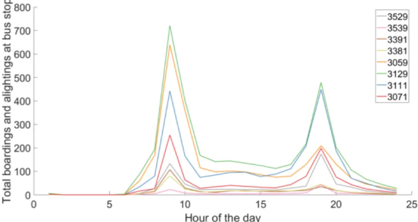
Finally, we need to know how many people board and alight the buses for different types of the day. This is needed to estimate the dwelling duration of the buses at the bus stops. We utilize the tap-in tap-out dataset from the LTA data mall to extract the inbound and outbound average trip counts at the stops of interest (fig. 14)

Intersection controllers positions and phases:

We chose to position traffic lights only at intersections that include two roads with more than 1 lane per direction in order to facilitate the traffic flow through the area. A total of 4 traffic light-controlled intersections were defined at the positions indicated at fig. 13b. The timings of the different phases were manually tuned to maximize the flow of vehicles through the intersection at rush hour traffic conditions.

Vehicle population parameters:

(24)

(a) The routes of the bus lines are marked with either yellow (standard road segment along the road or red (road segment on which there is a bus stop).

(b) Locations of signalised intersections (indicated in red)

For the purposes of this study we have assumed that the vehicle population consists of private vehicles and public transport buses. The physical properties of private vehicles are modelled after the Toyota Corolla Altis since it is one of the most commonly used vehicles in Singapore.

The bus population is split into a 2:1 ratio between single and double deckers. The electric equivalent of the chosen private vehicle is the Nissan Leaf.

3.3.2.2 Simulation Model

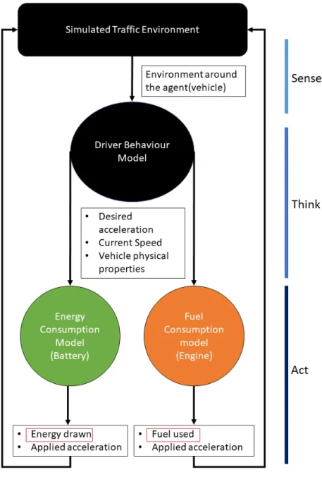
CityMoS is a time-stepped agent-based simulator, which means that at every time step of the simulation (0.25s) every agent (vehicle) performs three actions.

• Sense: Receives information from the simulation engine about the positions, velocities, accelerations of the vehicles around it and about the physical properties of the accessible road network system.

• Think: Based on the information gathered during the sense step and the objectives such as route to follow, mandatory lanes to be on, bus stops to visit etc. the driver behaviour models decide what should be the next actions of the agent. The actions describe the lateral and longitudinal acceleration the agent wants to apply as well as the initiation of any lane changing maneuvers.

• Act: In the act phase, the simulation engine applies the actions that all agents chose to perform to the environment. This includes, most importantly, moving the agents but also updating all agents properties accordingly.

This process is visually depicted in fig. 15.

(25)

Figure 14: Volume of commuters boarding or alighting at bus stops throughout the day.

Since we are interested in the energy consumption of the agent, the most important update is the fuel consumption / battery update (depending on whether the agent is an ICE vehicle or an EV). In this particular update, the respective model takes as input the desired acceleration and computes the acceleration that the vehicle is physically capable of applying. After that, based on the current state of the vehicle, the model computes how much energy would be needed to apply this acceleration. In the case of ICEs, this includes an engine model that computes RPM values and gear changes. In the case of EVs the model computes the required power and whether the motor can provide it.

3.3.2.3 Simulation Outputs and Post-processing

The raw output of the mobility simulation is the energy consumption/heat and coordinates of every vehicle for every time step of the 24 hour simulation period. In order to incorporate these results into the microclimate simulator these point heat emissions need to be aggregated in time and space. The time aggregation is on an hourly basis while the spatial aggregation is based on the cell boundaries defined by the climate simulator domain. We have assumed that all heat emissions from traffic occur at the same vertical level, which means that the spatial aggregation problem is solved in two-dimensional space. In other words, the post-processing of the raw data produces 24 heat emissions profiles, one for every hour of the day, where all raw heat emissions within this hour are grouped based on their positions into the domain cells near the ground surface. The total energy in each cell is divided by the cell area and by the duration of the time period (1 hour) in order to produce a heat flux inW/m².

The heat flux Ci,t at cell with id iduring time periodtis formalized as:

C_i,t=

P

j∈S_i,t−1<τ≤t

h_j,τ

Area(C_i)T , (10)

whereh_j,τ is the heat released at positionj at timeτ in Joules,S_i is the set of points that belong to celli,Area(C_i)is the area of celliin m², andT is the duration of one time period

(26)

Figure 15: Simplified workflow of traffic simulator

in seconds.

(27)

3.3.3 Microclimate

There are several methods that can be used to assess the urban microclimate. These include field measurement, wind/water tunnel experiment, and computer fluid dynamics (CFD). The selection of the appropriate method is mostly determined by the objective of the study. In this case, CFD simulation is chosen since it is not only able to provide data at high-resolution, it also takes into account the two-way relationship between urban features and climatic conditions.

We carried out a CFD simulation with ANSYS Fluent 18.2 [23], one of the most widely known CFD modeling tools [24–26].

3.3.3.1 Governing Equations

The governing equations for finite volume incompressible flow are the three laws of

conservation, i.e. Conservation of mass (Continuity), conservation of momentum (Newton’s second law) and conservation of energy (First law of thermodynamics). In CFD, these laws are generally named the Navier-Stokes (NS) equations. To directly solving the NS equations for high-Reynolds number flows is prohibitively expensive. Therefore, the approximate forms of these equations are solved. In urban physics, Reynolds-Averaged Navier-Stokes (RANS) equations are often used and are derived by averaging the NS equations. The RANS model does not directly compute any turbulence by NS equations but approximates the turbulence flows. It is done by decomposing solution variables appeared in the instantaneous NS equations into a mean and fluctuating component:

f =f +f⁰ (11)

wheref is the instantaneous value of variables,f is the mean value, andf⁰ is the fluctuating value.

In this study, 3D double precision with pressure-based solver, and the steady RANS equation is used for all the simulations. The simulation is running on a Linux platform with 32 processors which took about 12 hours for each run.

The governing equations are expressed as:

Continuity equation:

∂u_i

∂xi

= 0 (12)

Momentum equation:

uj

∂ui

∂xi

=−1 ρ

∂p

∂xi

+µ ρ

∂²ui

∂xi∂xj

− ∂

∂xj

(u⁰_iu⁰_j) +fi (13)

(28)

Heat conservation:

ui

∂T

∂xi

+ ∂

∂xi

(KT

∂T

∂xi

) = 0 (14)

whereu_i is the average wind velocity,ρis the density of air,u⁰_iu⁰_j is the Reynold stress,µis the molecular viscosity,f_i is the thermal-induced buoyant force,T is the potential

temperature, K_T is the heat diffusivity.

Turbulence Modelling With RANS equations, only the mean flow is solved while all scales of the turbulence are modelled using approximation. This approximation by the turbulence modelling can considerably reduce the computational cost and makes it feasible to simulate complex high-Reynolds number flows. The turbulence modelling is classified in terms of number of transport equations solved in addition to the RANS equations, such as zero equation model (e.g., Mixing length, Cebeci-Smith), one equation model (e.g.,

Spalart-Allmaras, k model), two equation model (e.g., k-ε, k-ω), etc.

In this study, Realizable k-εturbulence model is chosen. This model is one of the models that is commonly used in the urban physics studies. The model is known for its good performance in separated flows and those with complex secondary flows (Han, 2005). It is also good for modelling flows that involve high shear or separation commonly found in urban simulation (DeBlois et al., 2013).

The two equation Realizable k-εmodel gives a general description of turbulence by means of two transport equations, as follow:

• Transported variable is the turbulent kinetic energy (k).

• Rate of dissipation of turbulent kinetic energy ()

Heat Transfer Heat transfer describes the flow of thermal energy from one substance or material occupying one region in space to another substance or material occupying different region in space. In this study, the heat transfer modelling includes radiation, conduction and convection. In CFD simulation, energy equation is used to compute the heat fluxes and produce the temperature field.

A Radiation model can be included to take into account heating or cooling of surfaces due to radiation and/or heat sources or sinks due to radiation within the fluid phase. The Direct Ordinates (DO) model is one of the most comprehensive radiation models provided in ANSYS Fluent. This model accounts for reflected, absorbed, emitted and scattered radiation. The DO model uses the basic Radiative Transfer Equation (RTE), but rather than solving the infinite number of directions of the beam occurring at a point in space, DO model only solves for a discrete number of beam directions. For the solar load settings, the sun direction vector is set using solar ray tracing method for fair weather conditions. The solar radiation

parameters, such as direct and diffuse irradiation, uses the same weather data as 3.3.1.1.

For natural convection problem, buoyancy is considered using the Boussinesq Approximation.

Natural convection occurs when heat is added to a fluid and the fluid density varies with

(29)

temperature, a flow can be induced due to the force of gravity acting on the density variations. The Boussinesq model assumes the density as a constant value in all solved equations, except for the buoyancy term in the momentum equation [23].

(ρ−ρ₀)g≈ −ρ0β(T −T₀)g (15)

3.3.3.2 Simulation Settings

Meshing and Domain Configuration In CFD, the accuracy and reliability of the simulation output can be determined by several factors, two of the most important ones are the mesh quality and domain configuration. We followed the best practice guidelines by the Architecture Institute of Japan (AIJ) [27]. The domain size is 5000 x 5000 x 2100 m for all the simulation cases, which satisfies the minimum distance requirement of a domain of at least five times the height of the tallest building (5H) from the edge of the urban 3D model to the inlet and outlet, and minimum of 5H from the highest building to the top of the domain. The overall blockage ratio in the streamwise direction is less than 3%. These requirements are necessary to make sure that the domain is big enough for the flow field to be fully developed before reaching the urban area.

Figure 16: Domain configuration

The mesh quality is also critical to the accuracy of the result. For studies that are focusing on the pedestrian level wind speed, it is recommended to have at least three or four layers from the ground surface to the observation height (i.e., 1.5 – 2 meters). The structured hexahedral mesh is selected in this study with the growth ratio of 1.3 for all the simulations. The total cell

(30)

Table 2: CFD Domain Configuration

Study area 800 x 800m²

Highest building 350 m

Domain size (l x w x h) 5000 x 5000 x 2100 Minimum cell size 0.5 m (vertical)

Growth ratio 1.3

Number of cells 13 - 24 million

Blockage ratio < 5%

count ranges between 13-24 million cells depending on the scenarios. We performed the mesh independence study prior to the real simulation work to determine the right mesh resolution.

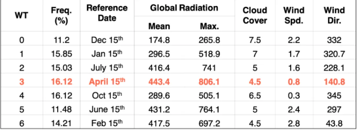
Input Boundary Conditions The weather data of 2016 from MSS Singapore is obtained from the nearest weather stations and implemented as the input boundary condition. Rather than simulating the case for the entire year, which can be very time consuming and

computationally very expensive, we categorized the typical Singapore weather within a year using a clustering and statistical method [28]. We identified seven typical Singapore weather types (WT), as shown in table below:

Figure 17: The typical weather types (WT) in Singapore using clustering method by Acero, et.

al. (2019).

In this study, we selected WT 3 which has the highest solar radiation intensity and low wind speed. The wind profile and aerodynamics characteristics of the flow (e.g., turbulent kinetic energy (k) and epsilon (ε)) was derived from the 1D wind profile generated by ENVI-met software using the same weather data. A similar method is already implemented in the ref [29]. In the latest version of ENVI-met (ENVI-met version 4.4), there is no feature to include the AH fluxes as the input data, hence the active strategies in this project are simulated with ANSYS Fluent.

The example of the wind profile at 6:00 AM is shown in fig. 18.

(31)

Figure 18: The example of wind profile at 6:00 hrs, obtained from 1D ENVI-met boundary condition.

In the simulation domain, we also implemented the soil layer that acts as the thermal balance as one of the key elements of urban energy balance. The ground plane in ANSYS Fluent is modelled explicitly as a 4.5 meters deep of soil layer to match ENVI-met’s model. A similar method of adding soil thickness in ANSYS Fluent modelling has been implemented in previous urban climate studies (Bottillo, Vollaro, Galli, and Vallati, 2014a; Y. Toparlar, B.

Blocken, B. Maiheu, and G. van Heijst, 2018). In this experiment, the soil model includes 0.3 meter asphalt and 4.5 meters loam, as shown below. Soil temperature at 4.5 meters depth was set as constant at 28.81^oC.

The other important key parameter for the simulation settings is the correct roughness parameter needed for the wall and the ground surfaces. For the wall roughness, the following equation is used:

k_s=9.793z0

C_z (16)

whereks is the equivalent sand-grain roughness height,z0 is the aerodynamic roughness length andCzis the roughness constant.

(32)

Table 3: CFD simulation settings Simulation Parameters Details

Solver type Pressure-based, RANS steady state

Dimension 3D

Turbulence model k-ε

Wall function Standard wall function

Radiation model Direct ordinates

Solar load model Solar ray tracing method Global position 103.85^o E, 1.27^oN

Timezone (GMT) +8

Simulation date 15 April (WT 3)

Simulation time 24 hours

Pressure-velocity coupling SIMPLE method Spatial discretization

Gradient Least squared based cell

Pressure Body force weighted

Momentum Second-order upwind

Turbulent kinetic energy Second-order upwind Turbulent dissipation rate Second-order upwind

H2O Second-order upwind

Energy Second-order upwind

Relaxation factors Default

Convergence criteria 1E-5, energy equation 1E-6

Initialization method Hybrid

Number of iterations 5000

3.3.3.3 Heat Source Setup

District Cooling and Cooling Tower: Both the cooling tower and DCS generate AH in two forms, sensible and latent heat. For the cooling tower scenario, the heat is released at the rooftop of every building, while in the DCS scenario, the heat is only released from the selected roof area where the DCS plans are located. As latent heat is not available as direct input, it then must be modelled as the flow of humid air. To produce the properties of this humid exhaust air, we computed the operation based on the cooling tower energy balance.

This model solves the state of exhaust air as well as other important information, such as number of fans and the dimension of the fan outlet/opening (See section 3.3.1.1. In the CFD simulation, we selected mass-flow-inlet as the heat source boundary condition to release this hot humid air into the domain. The input conditions needed are the mass flow rate, rejected temperature, air velocity for every system in hourly resolution.

Mini-split Unit: Unlike the cooling tower and DCS, a mini-split unit releases the heat in 100% sensible form and the heat source is located on the building wall. In reality, a mini-split unit is commonly used for residential and the outdoor units, where the heat gets rejected to the outdoor spaces, are arranged in vertical lines attached on the building’s exterior walls. To increase the accuracy of the result while also keeping the number of cells as low as possible, the heat source for mini-splits is designed as stripes along the building wall with one meter

(33)

Figure 19: Example of the heat rejection points for AH emission generated from cooling tower (left), and example of the heat rejection points for AH emission generated from DCS (right)

width for each. The number of the stripes represents the number of residential units in every floor, with assumption that the average of apartment unit in Singapore is 10 meters wide [30].

Traffic: As the microscopic traffic simulation is able to produce the output in a relatively high resolution in terms of time and space, we decided to map the heat intensity output directly into CFD simulation. The pointwise heat emission is produced based on the ANSYS meshing in an hourly resolution. The heat intensity is generated for every cell within the area we identified as the road surface. The heat generated from transportation is assumed to be generated in 100% sensible form.

Figure 20: Example of the heat rejection points for AH emission generated from minisplit unit (left), and example of the heat rejection points for AH emission generated from transportation (right)

(34)

3.3.3.4 Simulation Output

Microclimate modelling using CFD simulation provides the climatic variables (i.e., wind speed, air temperature and relative humidity) that can be further post-processed to assess the impact of AH fluxes that are generated from a number of different active strategies on

microclimatic condition. Each variables is extracted in hourly resolution for the 24-hour period within the target area (i.e., 75% study area) as shown in Figure 21. The rest 25% of study area is treated as surrounding buildings to induce enough turbulence for the target area. Hence, 25% of the area is not considered in the analysis. To understand the magnitude of AH impacts in the outdoor environment, we cross-compared the outputs of cases with and without AH (i.e., Baseline case).

Figure 21: Only the 75% of the study area (i.e., target area) is included in the analysis while the remaining 25% is needed to induce sufficient turbulence for the urban flow conditions.

Due to the high computational cost of CFD simulation, we focus the analysis on the most extreme technology scenarios for transportation and buildings. These extreme scenarios could help us to understand the maximum potential of the new alternative technologies, as

compared to the business-as usual. Table 4 shows all the cases that are simulated and analysed with CFD.

AH dispersion depends on the location of heat rejection, magnitude and the form of heat that is being rejected. When AH is released into the outdoor spaces, it could alter the temperature and flow field. Subsequently, the changes in the flow field would affects the dispersion of AH.

This can be clearly seen in AH building scenarios, as shown in Figure 22 and Figure 23.

The graphs are plotted from the output at 5:00 hrs, hence the changes in the wind and temperature field are only caused by AH, and no influence from solar radiation. In the

(35)

Table 4: CFD simulation cases.

Case AH Building AH Transportation

Baseline (No-AH) N/A N/A

B-BAU (Buiding-Scenario 1) Cooling Tower system for Commercials and Mini-plit Unit for

Residential buildings. N/A B-DCS (Building-Scenario 4) 100% District Cooling

System for Commercials

and Residential buildings. N/A

T-BAU (Transport-Scenario 1) N/A 100% Internal Combustion

Engine (ICE) both for private cars and public buses.

T-EB (Transport-Scenario 5) N/A ICE for private cars

and 100% electric bus.

T-EV (Transport-Scenario 4) N/A 100% electrification for both private cars and public bus.

baseline case (No-AH), there is no change in the temperature and the turbulence is only governed by urban geometry. When AH is released from mini-split unit (Scenario B-BAU, nighttime), sensible heat is discharged from the condenser, which is normally attached on the building exterior wall hidden from the main road. This direct exposure of AH into the street canyon increases the air temperature near the mini-split condenser unit by about 1-1.5^oC.

The flow field is also changed when AH is released. The buoyancy force causes the hot air to rise to the roof level, allows the heat exchange at the top and induces the cooler air to enter from the top as well as from the sides of the building blocks.

For centralised cooling tower (Scenario B-BAU, daytime) and DCS (Scenario B-DCS), both systems release AH in the form of latent and sensible heat. From these cooling systems, latent heat adds moisture into the atmosphere, while sensible heat can directly alter the air

temperature of the surrounding area. But, most of the heat is normally discharged in the form of latent heat, the increase in temperature that is caused by sensible heat is rather minimum (see fig. 8).

In the cooling tower (Scenario B-BAU), AH is rejected from the roof of the building, which can be slightly above the UCL. Hence, the heat mostly affects the upper level of the domain, mostly in RSL (see section 1.2). From the contour plot, most of the heat is directly

transported to downstream area. Hence, the chance for the heat to be re-circulated into the UCL and reach the pedestrian level is very small. With the DCS system, AH is released from the district cooling plant, that is normally around tens of meters above the ground. In this study, the height of the DCS plant is between 20-30 meters, which is within the UCL. Each one of the DCS plant covers several numbers of buildings, therefore, the magnitude of AH from one DCS plant is higher than one cooling tower system, but it is concentrated in one specific area. This caused a maximum air temperature increase of around 9^oC, adjacent to the heat source.

(36)

Figure 22: Air temperature distribution for AH building scenarios as compared to the Baseline (Non-AH scenario) at vertical plane.

The result for transportation scenarios is shown in fig. 24 and 25. These figures are plotted at 20:00 hrs, when there is no solar radiation. Therefore, the temperature changes are only caused by AH flux input from vehicles, since in all the transportation scenarios, heat released from buildings is neglected (see table 4). In the T-BAU scenario, the temperature increase on the road areas varies between 1-1.8^oC and the maximum increase is found at some spots in the sidewalk (up to 3^oC). The heat fluxes released from the vehicles also induces the thermal-driven-wind due to buoyancy. These effect increases the overall wind speed within the street canyon, as shown in fig. 25. With the electrification strategies (i.e., electric bus in scenario T-EB and full electrification in scenario T-EV), a lower temperature increase can be observed in the street canyon in comparison to the case T-BAU. Scenario T-EV shows relevant benefits with a minimum air temperature increase in certain hot spots. As the AH input decreases with the electrification strategy, the air temperature increase reduces as well as the buoyancy effect. The wind speed is calmer in T-EV, compared to scenario T-EB and T-BAU.

(37)

Figure 23: Wind speed distribution for AH building scenarios as compared to the Baseline (Non-AH scenario) at vertical plane.

3.4 Assessment

This section describes the metrics used to assess the impacts of technology scenarios (Section 3.2) on the urban outdoor environment.

3.4.1 Final Energy Consumption

Final energy consumption is the total energy consumed by end-users such as vehicles and buildings, including district cooling. No further energy losses and consumption in upstream processes are included. There are three sources of energy relevant to the case: electricity, gasoline and diesel. For fuels, we quantify the energy content via the Lower Heating Value

(38)

Figure 24: Air temperature distribution for AH Transportation scenarios as compared to the Baseline (Non-AH scenario) at vertical and horizontal plane (2 m above ground).

(LHV).

The reporting unit is final energy (electricity and fuel) consumed per year [GWh/ yr] (lower is better).

The metric is calculated by the simulation models CEA (buildings and district cooling) or CityMoS (ICEVs and EVs).

3.4.2 Green House Gases

Electricity production and ICE vehicles are major sources of GHGs, which contribute to climate change and include CO2, CH4, N2O and fluorinated GHGs. The cases can thus be evaluated in terms of these emissions, which for simplicity we limit to emissions within Singapore and during their operation phases. These emissions include those of buildings and district cooling via their electricity consumption, and those of transportation via both electricity and motor fuel consumption.

GHGs have different warming effects, but these can be unified by using the 100-yr global warming potential (GWP100) as adopted in the UNFCCC [31].

The reporting unit is thousand tonnes of equivalent CO2 emissions per year [kT CO2e/ yr]

(lower is better)

(39)

Figure 25: Wind speed distribution for AH Transportation scenarios as compared to the Baseline (Non-AH scenario) at vertical and horizontal plane (2 m above ground).

Assumptions and emission factor calculations:

Electricity: Grid emission factors for direct CO2 and fugitive CH4 emissions are

available [32]. Although the fugitive emissions of natural gas, which is responsible for about 95% of Singapore’s electricity [33], refer to any CH4 emissions in the upstream infrastructure (from extraction to delivery to power plants), we assume that the quoted fugitive emissions are for infrastructure in Singapore. These two components account for 99.7% of the GHG intensity of electricity, but for completeness, we also included the direct CH4 and N2O emissions using the Tier 1 (default) emission factors of fuels [34] and data from the Singapore Energy Statistics [33] (we further assume that the ‘others’ generation fuel refers solely to municipal solid waste, with a 1:1 biomass and non-biomass proportion). Due to the significant use of cogeneration plants in Singapore, using the Tier 1 CO2emission factor leads to 14.1%

more emissions compared to the official grid emission factor; this considerable difference was used as an allocation factor to separate the emissions of electricity and cogeneration heat production. GWP100 values were used in [31].

Gasoline and Diesel: Similarly, we calculated the direct CO2, CH4 and N2O emissions based on Tier 1 (default) emission factors, and weighed by GWP100. We exclude any

emissions upstream of the vehicles for simplicity, which is complicated by the mix of imported and domestically refined fuels.

(40)

Calculation: The emissions due to energy usageEi is typically calculated by way of an emission factorphii whereiindicates whether the emission factor is for electricity (e), gasoline (g), or diesel (d) as in Eq. (17). For electricity, the emissions factor considers the typical grid loss of 3% [35]on top of the standard reported emission factor (this is reflected in the table).

The emission factors are shown in Table 5, and the results are scaled to an annual basis.

Emissions= X

i∈e,g,d

E_i·φ_i (17)

Table 5: Emission factors electricity 0.5 kg CO2e/kWhgenerated

gasoline 72.12 kg CO2e/GJ LHV diesel 75.24 kg CO2e/GJ LHV

3.4.3 Canopy-layer Temperature

Urban Canopy Layer (UCL) is the lower level atmospheric layer that is dominated by

microscale processes due to urban elements, surface properties and spatial arrangements. The height of canopy layer is measured from the ground to the mean height of buildings or trees (Oke, et al., 2017).

The height of canopy layer in this study is calculated by:

HU CL=

n_b

X

i=1

hiwi,

w_i= A_i

n_b

P

i=1

A_i

(18)

whereHi is the height of the toweriin metres,nb is the number of towers in the target area, andw_i is the weight that is calculated from the ratio of footprint area of the toweri(A_i) and the total areas of all the towers within the target area.

Then, the canopy layer temperatureT_{U CL}is derived by:

T_z_i = 1 n(x, y, zi)

X

x,y∈Area

T(x, y, z_i) (19)

TU CL= 1 n₍zi)

nh

X

z_i=1

Tz_i (20)