Investment Strategies of German Households in a Multi-layer Portfolio Framework
228
0
0
Volltext
(2)
(3)
(4)
(5)
(6)
(7)
(8)
(9)
(10)
(11)
(12)
(13)
(14)
(15)
(16)
(17)
(18)
(19)
(20)
(21)
(24)
(25)
(27)
(28)
(30)
(31)
(32)
(33)
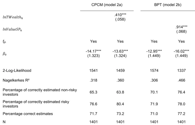
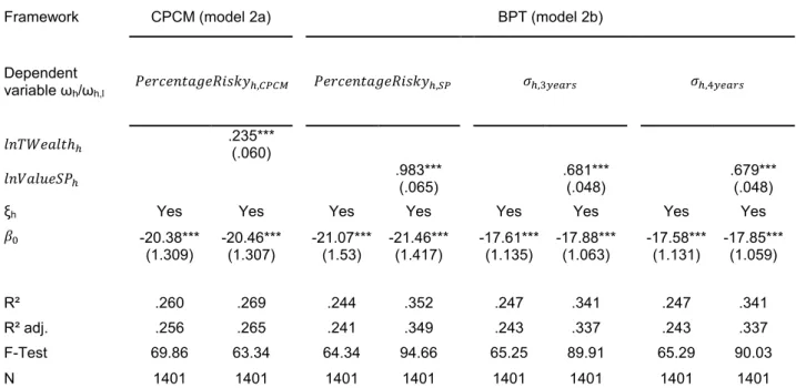
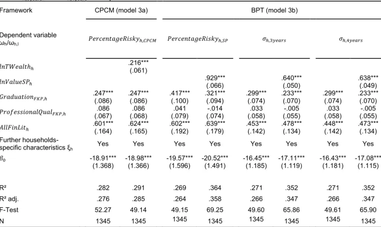
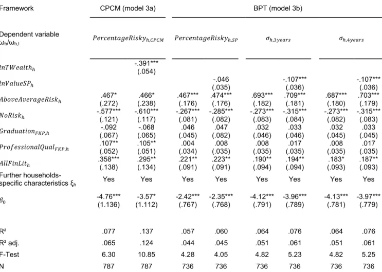
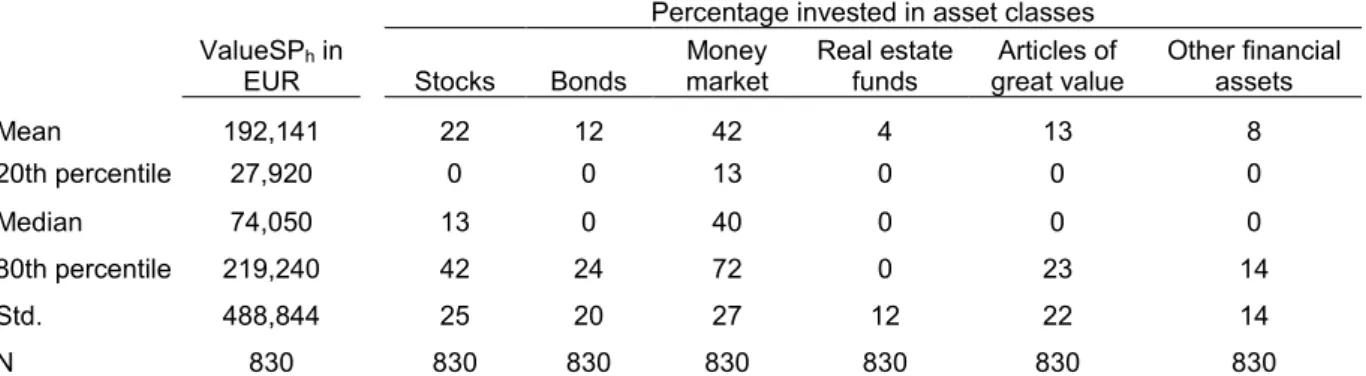
Abbildung
+7
ÄHNLICHE DOKUMENTE
Beside these applications, which focus on prediction of structural change, the models of continuous dynamics discussed in our paper have further applications in in structural
The FVA is a set of rules, components, standards and protocols that together make up a framework (FVA) to ensure that all internationally transferred mitigation
In rice production in the Philippines for example, it has been observed that higher quality land is inversely related to the size of the farms under share tenancy contracts
The first part (Chapter 2, “Access to Banking and its Value for SMEs - Evidence from the U.S. Marijuana Industry” and Chapter 3, “Contemporaneous Financial Intermediation - How
Figure 1 (b) shows the lower bound for relative negotiation costs as a function of financing spread, such that a firm’s management chooses the shortest negotiation process at least with
We test our model using a data base from a German bank’s tick-by-tick end-user order flow and respective quotes and find that financial customers exert massive market power
In this paper, dynamic responses of the sticky information Phillips curve and a standard sticky price Phillips curve to a unit cost-push shock 3 are investigated and compared in a
The predicable component of information asymmetry, which can be attributed to the skilled analysis of public information, differs from the private firm-specific
