An Exact, Fast Algorithm for the "Charge Refinement Problem" in the Simulation of Heavy-Ion Collisions, in Comparison to Slimmed-Down Neural Networks

Helmut Hörner

An Exact, Fast Algorithm

for the "Charge Refinement Problem"

in the Simulation of Heavy-Ion Collisions, in Comparison to Slimmed-Down Neural Networks

Project Report

Version 3

Vienna University of Technology Institute of Theoretical Physics

Vienna, November 2019

Abstract

In certain numerical simulations of the early stages of heavy-ion collisions it is necessary to split charges in Wigner-Seitz cells into smaller sub-charges, which are then smoothly distributed as to approximate a continuous charge distribution. "Smooth" means that the discrete fourth derivate should be constant within each Wigner-Seitz cell. In this paper, we demonstrate that simple, dense neural networks can be trained to learn this charge distribution task, and how these networks reveal the linearity of the problem.

We derive a very fast linear algorithm for directly calculating the exact charge distribution without

neural networks, and present a C++ implementation of this algorithm. Eventually, we go back to

neural networks and present more refined convolutional network architectures with a significantly reduced

number of trainable parameters. Because of their lean structure, these refined networks are a good

alternative to the exact solution when it comes to a very large number of charges.

Contents

1 Introduction 5

2 The Deep Learning Approach 6

2.1 Generating Training Data with the Original Iterative Algorithm . . . . . 6

2.1.1 Theory . . . . 6

2.1.2 Implementation in Python . . . . 10

2.2 Exploration of Multiple Deep Learning Configurations . . . . 11

2.2.1 Implementation in Python . . . . 11

2.2.2 Results . . . . 14

3 The Linear Algebra Approach 16 3.1 From Deep Learning to Linear Algebra . . . . 16

3.2 The Exact Linear Solution . . . . 18

3.2.1 Exact Solution for Constant Second Derivative . . . . 18

3.2.2 Exact Solution for Constant Fourth Derivative . . . . 23

3.3 Implementation in C++ . . . . 27

3.3.1 Passing and Retrieving Charges in C++ Arrays . . . . 28

3.3.2 Passing and Retrieving Charges in Vectors . . . . 29

3.3.3 Passing and Retrieving Charges One by One . . . . 30

3.3.4 Retrieving Matrices M ₁ and M ₂ . . . . 31

3.3.5 Generating Matrix Files by Command Line Parameter Calls . . . . 32

3.3.6 Explanations to the Charge Refinement Class Core Function . . . 34

4 Back to Neural Networks 35 4.1 Can Matrix M ₂ be Retrieved From a Trained Neural Network? . . . . 35

4.2 Retrieving Matrix M ₂ More Directly From a Neural Network . . . . 40

4.3 Retrieving Matrix M ₂ Most Directly . . . . 42

4.4 Simple Convolutional Networks . . . . 44

4.4.1 Theory . . . . 44

4.4.2 First Implementation in Python . . . . 45

4.4.3 Results . . . . 49

4.5 Improved Implementation in Python with Handling of Boundary Charges 51 4.5.1 Results . . . . 51

4.6 Better Results with Less Neurons . . . . 54

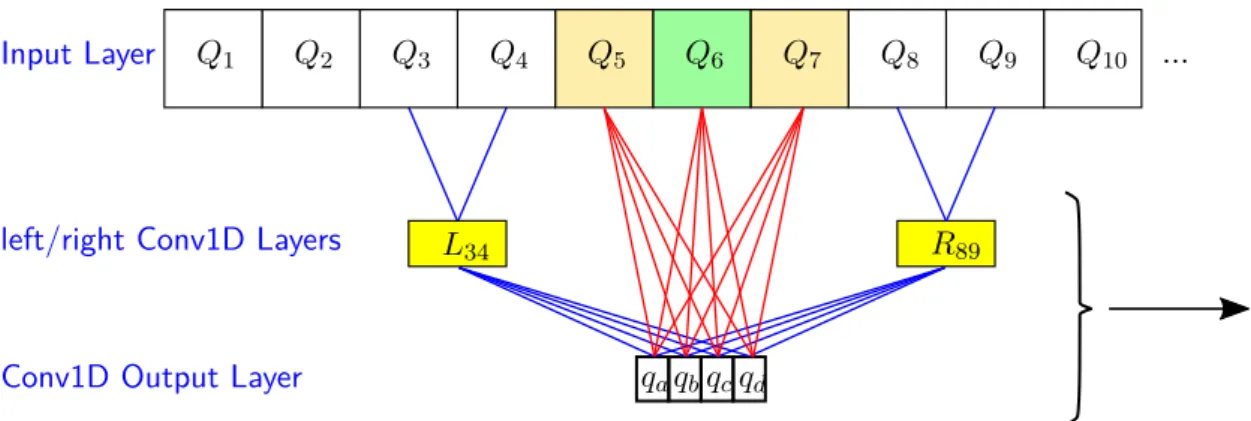
4.6.1 A Refined Architecture - The Basic Idea . . . . 54

4.6.2 The Actual Implementation . . . . 55

4.6.3 Results . . . . 59

4.7 Further Slim Down the Neural Net . . . . 61

4.7.1 Exploiting Mirror Symmetry . . . . 61

4.7.2 The Actual Implementation . . . . 62

4.7.3 Results . . . . 65

5 Conclusions 67

6 Appendix 68

6.1 Listing "Charge Refine Train Data Generator" . . . . 68

6.2 Listing "Charge Refine Deep Learning Explorer" . . . . 70

6.3 Listing "Charge Refinement Class" . . . . 73

6.3.1 Header File . . . . 73

6.3.2 clsChargeDistr . . . . 74

6.4 Convolutional Network with Handling of Boundary Charges . . . . 82

1 Introduction

In [Gelfand et al, 2016], a numerical simulation of the early stages of heavy-ion colli- sions in 3+1 dimensions is presented. It makes use of the nearest-grid-point (NGP) interpolation method [Moore et al, 1998], where a particle charge Q(t) at a specific time t is fully mapped to the closest lattice point. The charge density only changes when a particle crosses the boundary in the middle of a cell such that its nearest-grid-point changes. These boundaries can be formally defined with a Wigner-Seitz lattice, with lattice points marking the center of each cell.

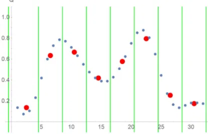
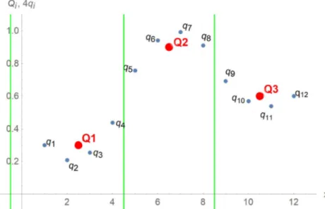
However, for the simulation not to produce a lot of numerical artifacts, it is crucial to approximate a continuous charge distribution. Therefore, it is not sufficient to represent the total charge per Wigner-Seitz cell with a single charge. Instead, in each Wigner- Seitz cell the total charge must be split into smaller sub-charges, which are then smoothly distributed as to approximate a continuous charge distribution (see Figure 1).

Figure 1: Originally, the total charge in each Wigner-Seitz cell (green lines) is repre- sented by a single charge (red dots). By splitting these single charges into multiple charges (blue dots), and distributing them so that the discrete fourth derivative is constant within each cell, a continuous charge distribution can be approximated. Please note that the refined charges (blue dots) are plotted with four times their actual values to better set them in visual context with the original charges (red dots).

In this context, "smooth" means that the discrete fourth derivate should be constant

within each cell. In [Gelfand et al, 2016], a (rather slow) iterative algorithm was imple-

mented to simulate such a charge distribution.

The initial goal of this project was to find out to what extent a deep-learning neural network could be trained to speed up this charge distribution task, and (if possible) to provide such a trained network.

As we will show in the following chapter 2, it turned out that (i) Deep networks can be trained to fulfill this task;

(ii) the fewer layers a network has, the better it works for this job;

(iii) so that, eventually, not-at-all-deep dense networks with no hidden layers work best;

(iv) and, additionally, such simple networks provide the best results if any non-linear activation function is abandoned in favor of a simple linear activation function.

Such an extremely simplified neural network can (because of its linear activation func- tion) be represented by a simple linear vector/matrix equation. Therefore, the problem can obviously be reduced to linear algebra. Consequently, we derived the exact linear solution, which we present later on in chapter 3.2, and a corresponding C++ implemen- tation in chapter 3.3.

Eventually, in chapter 4 we compare the weight matrix of a trained dense neural net- work with the exact solution, and further demonstrate how it still makes sense to use a convolutional network to quickly solve the charge-distribution problem for large charge distributions.

2 The Deep Learning Approach

2.1 Generating Training Data with the Original Iterative Algorithm 2.1.1 Theory

This chapter gives an overview of the iterative algorithm as presented in [Gelfand et al, 2016], that has been re-implemented by us in Python in order to gen- erate the training data set.

(1) Let Q _j be the total charge in the j-th Wigner-Seitz cell. In this first step we create N sub-charges q _i for each original charge Q _j , with N j ≤ i < N (j + 1). So, if we have, let’s say, 8 original charges Q 1 · · · Q 8 , and we decide to split each of these original charges into N = 4 sub-charges, then we get 32 sub-charges q ₁ · · · q ₃₂ , with sub-charges q ₁ , q ₂ , q ₃ , q ₄ being in the same cell as initially Q ₁ , sub-charges q 5 , q 6 , q 7 , q 8 being in the same cell as initially Q 2 , and so on. These sub-charges are then evenly distributed along the x-axes.

(2) Each of the sub-charges get the initial value q _i = ^Q _N

^j

for every N j ≤ i < N (j + 1).

So, in our example the initial values are set to q 1 = q 2 = q 3 = q 4 = ^Q ₄

¹

, q 5 = q 6 =

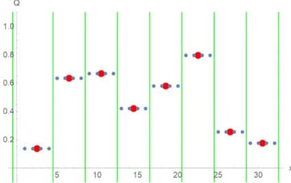
Figure 2: Initial distribution of the smaller sub-charges (blue dots). Please note that the sub-charges (blue dots) are plotted with four times their actual values to better set them in visual context with the original charges (red dots).

(3) This third step, if applied repeatedly, ensures that the discrete second derivative of the final distribution becomes constant. First, we randomly select a sub-charge q _i , excluding charges on the rightmost border of a cell from this selection process (i.e. excluding charges where i + 1 is a multiple of N ). We now want to find a value ∆q by which we modify q i → q ⁰ _i and q i+1 → q ⁰ _i+1 as follows:

q _i ⁰ = q i − ∆q (1)

q _i+1 ⁰ = q i+1 + ∆q (2)

This leaves the total charge in the cell unchanged.

After repeating this third step often enough, we want the discrete second derivative of the final distribution to be constant. Therefore, we expect that the gradient

q

i+1

−q

_i

∆x will eventually become the mean value of the left-side gradient ^q

ⁱ

^−q _∆x

ⁱ⁻¹

and the right-side gradient ^q

ⁱ⁺²

_∆x ^−q

ⁱ⁺¹

:

q _i+1 ^{f inal} − q _i ^{f inal}

∆x = 1

2

q ^{f inal} _i − q _i−1 ^{f inal}

∆x + q ^{f inal} _i+2 − q ^{f inal} _i+1

∆x

!

(3) As we don’t know the final values for all q i ’s yet, we have to use the following iterative equation in each iteration step instead:

q ⁰ _i+1 − q _i ⁰

∆x = 1

2

q i − q i−1

∆x + q i+2 − q i+1

∆x

(4)

All sub-charges q _i are evenly distributed along the x-axes, therefore we can multiply equation (4) with ∆x and get

q _i+1 ⁰ − q ⁰ _i = 1

2 (q i − q i−1 + q i+2 − q i+1 ) (5) Inserting (1) and (2) on the left hand side of equation (5) leads to

q i+1 + ∆q − q i + ∆q = 1

2 (q i − q i−1 + q i+2 − q i+1 ) (6) which can eventually be transformed into

∆q = q _i+2 − 3q _i+1 + 3q _i − q i−1

4 (7)

We use this ∆q to modify charges q i and q i+1 as shown in equation (1) and (2).

This whole step (3) is to be repeated until equation (3) is fulfilled for all q _i within the required margin, except for the case when q _i is the rightmost charge in a cell, and also except for all q i with i = 1, i = N − 1 or i = N, as we don’t have charges q ₀ , q _N+1 or q _N+2 available to insert into formula (7).

(4) This last step, if applied repeatedly, ensures that the discrete fourth derivative of the final distribution becomes constant. As before, we start by randomly selecting a sub-charge q _i , excluding charges on the rightmost border of a cell from this se- lection process. And, again we want to find a value ∆q by which to modify q i → q ⁰ _i and q _i+1 → q ⁰ _i+1 as shown in equations (1) and (2), thereby leaving the total charge in a cell always unchanged.

After repeating this last step often enough, we want the discrete fourth derivative of the final distribution to be constant. Therefore, we expect that the third order finite difference δ _i ⁽³⁾ will eventually become the mean value of the left-side third order finite difference δ _i−1 ⁽³⁾ and the right-side third order finite difference δ _i+1 ⁽³⁾ :

δ ^{(3)f inal} _i = 1 2

δ ^{(3f inal)} _i−1 + δ ^{(3)f inal} _i+1 (8) The third order final difference is defined as

δ ⁽³⁾ _i =

3

X

k=0

(−1) ^n−k n k

!

q i−1+k (9)

which can be resolved into

δ ⁽³⁾ _i = q i+2 − 3q i+1 + 3q i − q i−1 (10) By inserting this into equation (8), we get

q

i+2

− 3q

i+1

+ 3q

i

− q

_i−1

= q

i+3

− 3q

i+2

+ 3q

i+1

− q

i

+ q

i+1

− 3q

i

+ 3q

_i−1

− q

_i−2

2 (11)

Again, this is the set of equations for the final solution. However, as we don’t know the final values for all q i ’s yet, we have to use the following iterative equation for any randomly chosen charge q _i and its neighbor q _i+1 in each iteration step instead:

q

_i+2

− 3q

_i+1⁰

+ 3q

⁰_i

− q

_i−1

= q

_i+3

− 3q

_i+2

+ 3q

_i+1

− q

_i

+ q

_i+1

− 3q

_i

+ 3q

_i−1

− q

_i−2

)

2 (12)

Inserting (1) and (2) on the left hand side of equation (12) leads to

q i+2 − 3 (q i+1 + ∆q) + 3 (q i − ∆q) − q i−1 = q _i+3 − 3q _i+2 + 3q _i+1 − q _i + q _i+1 − 3q _i + 3q i−1 − q i−2 )

2

(13)

which can eventually be transformed into

∆q = q i−2 − 5q i−1 + 10q _i − 10q _i+1 + 5q _i+2 − q _i+3

12 (14)

We use this ∆q to modify charges q i and q i+1 as shown in equation (1) and (2).

This whole step (4) is to be repeated until equation (11) is fulfilled for all q _i within

the required margin, except for the case when q i is the rightmost charge in a cell,

and also except for all i < 3 or i > N − 3, as we don’t have charges q −1 , q 0 , q _N+1 ,

q _{N +2} or q _{N +3} available to insert into formula (14).

2.1.2 Implementation in Python

Appendix 6.1 shows our Python 3.6 implementation of the algorithm explained in the previous chapter. All source code line references in this chapter refer to that listing.

We used our implementation to generate 2,000,000 records of training data (defined in line 8), each record representing 8 original (coarse) random charges (defined in line 10) as training input for a neural network. Each original charge is then split into 4 sub-charges (defined in line 11), so that the resulting output consists of 32 smoothly distributed charges representing a target configuration to which the neural network is to be trained.

chrg_generator(n)

Generator chrg_generator(n) (lines 15-40) returns n training data sets, each contain- ing 8 original (coarse) random charges, and 32 corresponding refined charges. Refined charges are initialized to have the same value as the original charge in the same cell (line 24), which means that the division by 4 has been skipped in order to ensure that both original and refined have the same magnitude between 0 and 1 (with refined charges occasionally having values slightly below 0 or above 1).

Line 27-32: The first refinement step (ensuring that the discrete second derivative be- comes constant) is performed 50 times (each time on a randomly chosen charge), before the maximum deviation is checked. This step is repeated until all charges are within the chosen absolute deviation of 2.5 · 10 ⁻⁶ (as defined in line 13).

Line 34-39: The second refinement step (ensuring that the discrete fourth derivative becomes constant) is handled in the same way.

deviationOK(q, step)

Lines 41-51: Function deviationOK(q, step) receives an array q of refined charges, and returns true, if all charges are within the chosen deviation, i.e.: if all ∆q by which the charges should be readjusted are smaller than maxErr. The second parameter step defines whether the deviation is to be checked with regards to the first or the second refinement step.

refine(chrg, step, i=-1)

Lines 53-68: Function refine(chrg, step, i=-1) receives an array chrg of to-be-

refined charges. If parameter i is passed to the function, then the i-th and (i + 1)-th

charge is adjusted by ∆q. If parameter i is not passed, a charge in array chrg will be

randomly chosen. If the charge defined by i, or the randomly chosen charge, happens

to be the rightmost charge in a cell, then there are no modifications. This is ensured,

also in case where the charge in question happens to be a boundary charge not captured by the algorithm). Parameter step defines whether the refinement is to be done with respect to the first or the second refinement.

dq_func(chrg, i, step)

Lines 70-97: Function dq_func(chrg, i, step) corresponds to ∆q in the refinement algorithm. In its first parameter, it receives an array chrg of to-be-refined charges. The second parameter i defines which charge in the array (together with the neighboring charge i + 1) is to be modified. The last parameter step defines, whether ∆q is to be calculated with regards to the first or the second refinement step. If i defines a rightmost charge in a cell (line 82), or a boundary charge not captured by the algorithm (line 87 and line 93), then zero is returned.

Main Program

In lines 104-114, arrays train_data and train_targets are filled with random (coarse) charge distributions and corresponding refined charge distributions produced by gener- ator chrg_generator(n). Progress information is printed every 100 generated records.

In lines 116-122, the refined charges are re-scaled so that the re-scaled values never leave the range between 0 and 1, in order to match a typical value range for many neural networks’s output layer.

In line 124-138, the generated data is stored into two files train_data.pkl and train_targets.pkl.

2.2 Exploration of Multiple Deep Learning Configurations 2.2.1 Implementation in Python

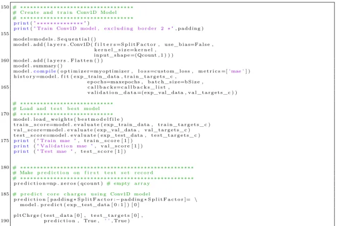
After having created the training data, we implemented the "Charge Refine Deep Learn-

ing Explorer", which is a piece of software for testing various Deep Learning models

against this training set. The Python 3.6 source code, utilizing Keras 2.2.4, is listed in

Appendix 6.2. All source code line references in this chapter refer to that listing.

Network Parameter Definition

In lines 14-20, some general network (meta-)parameters are defined, namely

• trainSetSize=1500000 ... defines the number of records from the created training set used for actually training the network

• trainSetSize=300000 ... defines the number of records from the created training set used for validating the network after each epoch

• testSetSize=200000 ... defines the number of records from the created training set used for testing the accuracy of the fully trained network.

• bSize=5000 ... in Keras, the batch size is the number of training examples in one forward/backward pass, i.e. the number of samples to work through before the internal model parameters are updated. The higher the batch size, the more memory space is needed.

• myoptimizer=’rmsprop’ ... this defines the optimizer by which the network’s weights are updated during the training phase. The selected optimizer uses "Root Mean Square Propagation", which is very commonly used and combines the the concepts of exponential moving average of the past gradients and adapting learning rate.

• maxepochs=2000 ... The number of epochs defines the number times that the learning algorithm will work through the entire training dataset. This parameter defines that training should stop after 2000 epochs at the latest.

• mypat=200 ... This defines the number of epochs after which training will be stopped prematurely if there is no further improvement.

Physics Parameter Definition

In lines 22-23, the parameters of the physics problem are defined, namely:

• numCells=8 ...This defines the number of Wigner-Seitz-cells), i.e. the number of (coarse) original charges in the training data set.

• pointsPerCell=4 ...This defines the number of (refined) sub-charges each original

(coarse) charge has been split into in the training data set.

createModel(nh1, nh2, nh3, nactfunc, actfuncin=True, actfuncout=False) Lines 31-77: This function creates and returns a dense deep learning model with up to three hidden layers. The size of the input layer is unchangeable and defined by the number of original charges numCells=8. Also, the size of the output layer is fixed at numCells*pointsPerCell (which is 32, in our case). However, the number and size of hidden layers is flexible and can be defined by passing parameters nh1, nh2, nh3 (defining the number of neurons in hidden layer 1, 2 and 3).

Parameter nactfunc may take on values between 0 and 10 and defines the network’s activation function (line 35-56). Parameter actfuncin is boolean (default: True), and defines whether the chosen activation function is also applied to the input layer (if it is False, then the input layer always has just a linear activation function). Boolean parameter actfuncout (default: False) does the same with the output layer.

plotToFile(history, round, step)

Lines 80-105: This function expects a History object as returned by Keras’ mode.fit method, and plots a graph of the training progress (training and validation loss) into a file. The integer parameter round just influences the file name (line 102), and reflects what number model has been tested. Finally, the integer parameter step may take on values between 1 and 4. If it is 1, then the whole curve is plotted. If it is 2, 3 or 4, then the first 10, 40, or 150 data points are skipped in the graphic.

MAIN PROGRAM

The main program starts at line 107. In lines 115-128, the complete training data set is loaded from the file. In line 130-140, the data set is split between actual training data, validation data and test data.

In lines 142-160, a log file is created, containing a header with general parameter infor- mation, and a headline for the information in the lines to come.

In lines 162-176, the number and type of the models to be tested are defined. The pa- rameters are the same as in createModel(...), namely nh1, nh2, nh3 as the number of neurons in hidden layers 1, 2 and 3 (zero for no layer), and nactfunc, actfuncin, and actfuncout to define which activation function to be used on what layers.

In lines 178-228, the actual simulations are executed, with the main loop starting in line

191. One by one, each model with parameters as defined before, is generated (line 195),

compiled (lines 196-197) and trained (lines 199-202). After that, the model is scored

against the test data set (line 205), and information is printed on screen and written to

the log file (lines 206-228). Eventually, in lines 230-236, graphs of the training progress

are plotted into files.

2.2.2 Results

In the first experiment, we ran multiple simulations with 1, 2 and 3 hidden layers, where the number of neurons in these layers were permutations of 4, 8, 16, 32, 64 and 128. In all these simulations we used the sigmoid activation function.

It turned out that all these networks could be trained to learn the training set, with mean absolute errors between 0.12 and 0.08 in less than 90 epochs (the patience parameter was set to 6 as to allow the simulations to end quickly for a fast screening of the various architectures). As expected, networks having a layer with just 4 neurons performed generally below average. Also, networks with one or two hidden layers performed better on average than networks with three hidden layers. It was also interesting that we never observed any overfitting.

In follow-up experiments we continued testing with network architectures that have proven to be above average in the first run. We increased the number of epochs (by setting the patience parameter gradually to higher values), and we also varied the activation function. It turned out that from all non-linear activation functions, the tanh-function performed best, followed by sigmoid, hard_sigmoid, and elu. With all other nonlinear activation functions the training results were non-satisfactory with the given architectures. Also, networks where input- and output layers did not have an activation function (i.e. had a linear activation function) performed better on average.

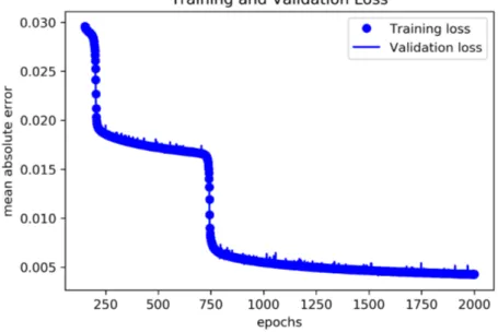
Figure 3: Training and validation loss (mean absolute error) development while train-

ing a dense deep network with 8-16-32-16-32 neurons and sigmoid activation

function over 2000 epochs.

In these experiments, a tanh-network with two hidden layers having 128 and 16 neu- rons, trained over 101 epochs, achieved the best mean average error of 0.004. However, a much simpler tanh-network with just one hidden layer with 8 neurons performed almost equally well with a mean average error 0.0052.

Although they are supposedly a core ingredient of deep learning architectures (see e.g.

[Goodfellow et al, 2016, p. 167])), we eventually decided to train networks where we have abandoned all non-linear activation functions in favor of the linear activation function.

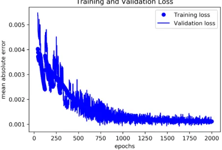
We also allowed for a network without any hidden layer. From all these networks, the most simple network, consisting of just 8 input and 32 output neurons (no hidden layers) performed best after being trained over 2000 epochs, reaching a mean average error on the test data of just 0.0011 (see Figure 4).

Figure 4: Training and validation loss (mean absolute error) development while training

a dense network with 8 input and 32 output neurons (no hidden layers) and

linear activation function over 2000 epochs.

3 The Linear Algebra Approach

3.1 From Deep Learning to Linear Algebra

Obviously, because of the linear activation function, the network from Figure (4), having just an 8-neuron input layer and a densely connected 32-neuron output layer, can be expressed in a simple vector/matrix equation.

Let Q ~ be the 8 ×1 input vector of (coarse) original charges. The first layer of the trained network can be represented by a 8 × 8 weight matrix W ₁ and a 8 × 1 bias vector ~b ₁ , so that the 8 × 1 output vector ~ o ₁ of the first layer can be written as

~

o ₁ = W ₁ Q ~ + ~b ₁ (15)

Let ~ q be the to-be-calculated 32 × 1 vector of refined small charges. We want this vector to be the output of the second layer. Like the first layer, the second layer of the trained network can be represented by a 32 × 8 weight matrix W 2 and a 32 × 1 bias vector ~b ₂ . As the output vector ~ o ₁ of the first layer is the input vector of the second layer, we can write

~

q = W ₂ ~ o ₁ +~b ₂ (16)

By substituting ~ o ₁ with the result from equation (15), we finally get

~

q = W ₂ W ₁ Q ~ + ~b ₁ + ~b ₂ (17) Considering that the split charges in the training dataset were not divided by 4, and further considering that the training dataset is re-sized (see source code lines 115-121 on page 69), the correct final formula is

~ q = 1

4





 2 W 2

W 1 Q ~ + ~b ₁ + ~b ₂ −





 0.5

.. . 0.5











 (18)

These are the actual matrices and vectors as retrieved from a trained network (rounded to five digits after the decimal point):

W

1

=





















−0.23201 −0.09500 −0.18980 −0.20857 −0.13743 −0.24721 −0.24588 −0.11497 0.83026 0.49651 −0.41574 −0.79812 0.18860 −0.10128 0.24538 −0.51374 0.81205 −0.35277 −0.01770 0.67868 0.02250 −0.03245 −0.89922 −0.43290 0.09440 −0.78898 −0.50042 0.31114 0.57818 −0.56365 0.67051 −0.07993 0.11048 −0.67576 −0.00760 −0.25418 −0.47597 0.71256 0.18709 −0.23155

−0.63754 0.13760 0.17649 0.03006 0.78638 0.45352 −0.10451 −0.99403 0.08440 −0.10035 0.95792 0.00775 −0.44585 −0.61243 0.42449 −0.57333 0.17292 −0.50736 0.67976 −0.76484 0.68332 −0.06788 −0.45818 0.48310





















W

2

=













































































































−0.37280 0.20164 0.17900 0.01525 0.02771 −0.13803 0.01954 0.04117

−0.39945 0.20787 0.21252 0.04556 0.07320 −0.15716 0.03436 0.07578

−0.38700 0.20508 0.19449 0.03114 0.05230 −0.14704 0.02970 0.06403

−0.33200 0.19186 0.12743 −0.03208 −0.04342 −0.10714 −0.00616 −0.01223

−0.25288 0.16871 0.02983 −0.12346 −0.18045 −0.04828 −0.05468 −0.12227

−0.19000 0.13716 −0.06000 −0.20229 −0.28451 0.01296 −0.06831 −0.17996

−0.16642 0.09801 −0.11750 −0.24235 −0.31373 0.05563 −0.02421 −0.14796

−0.18825 0.05178 −0.13084 −0.23736 −0.25991 0.07827 0.07031 −0.03150

−0.24450 −0.00152 −0.10079 −0.19346 −0.14884 0.07750 0.18644 0.11941

−0.30716 −0.06332 −0.04195 −0.13948 −0.03869 0.05886 0.26547 0.21186

−0.35718 −0.12917 0.03078 −0.09094 0.03198 0.02960 0.27786 0.19741

−0.38375 −0.19150 0.10322 −0.05402 0.04701 −0.00189 0.21986 0.08051

−0.38359 −0.23216 0.15648 −0.02019 0.00501 −0.02153 0.11643 −0.08960

−0.36382 −0.23266 0.17641 0.02562 −0.07015 −0.01709 0.01529 −0.21039

−0.33096 −0.18771 0.15776 0.08793 −0.15578 0.01560 −0.05169 −0.22978

−0.29522 −0.10675 0.10781 0.15693 −0.22899 0.07162 −0.07780 −0.14076

−0.26624 −0.01268 0.04364 0.20845 −0.26644 0.13593 −0.07638 0.01891

−0.25416 0.05250 −0.00209 0.20545 −0.24131 0.18271 −0.08259 0.16049

−0.26392 0.07117 −0.01775 0.13709 −0.15036 0.20022 −0.11219 0.23114

−0.29488 0.04434 −0.00560 0.01877 −0.00947 0.18593 −0.16472 0.21775

−0.34080 −0.00661 0.01843 −0.10938 0.14731 0.14910 −0.21340 0.12960

−0.38976 −0.04036 0.01966 −0.17844 0.26496 0.11097 −0.21785 0.02027

−0.43159 −0.03668 −0.01548 −0.15817 0.31318 0.08145 −0.16128 −0.07587

−0.45845 0.00338 −0.08588 −0.05457 0.28565 0.06325 −0.05388 −0.13660

−0.46171 0.05988 −0.16880 0.08889 0.20170 0.04714 0.06781 −0.15345

−0.43672 0.08876 −0.22419 0.19112 0.10253 0.01579 0.13800 −0.13051

−0.38573 0.06980 −0.23377 0.20978 0.01723 −0.03767 0.12797 −0.07540

−0.31756 0.00571 −0.19674 0.14598 −0.04022 −0.10870 0.04075 −0.00368

−0.24792 −0.07773 −0.13403 0.03791 −0.07191 −0.18034 −0.08090 0.06675

−0.20141 −0.13685 −0.08937 −0.03926 −0.08809 −0.22960 −0.16495 0.11670

−0.18958 −0.14830 −0.08119 −0.05286 −0.09633 −0.24031 −0.18200 0.13125

−0.21283 −0.12134 −0.10137 −0.01810 −0.08507 −0.21727 −0.14212 0.10492













































































































~b

1

=





















0.33668 0.03266 0.11375 0.14340 0.32480 0.07632 0.13475

−0.11565





















~b

2

=













































































































0.34976 0.33894 0.34399 0.36639 0.39867 0.42439 0.43396 0.42489 0.40172 0.37605 0.35625 0.34669 0.34708 0.35531 0.36727 0.38109 0.39280 0.39767 0.39366 0.38103 0.36234 0.34247 0.32567 0.31617 0.31504 0.32510 0.34581 0.37331 0.40058 0.41935 0.42426 0.41460













































































































Please note that the matrices and vectors printed above are not a unique, reproducible solution. Whenever re-trained, the network ends up with significantly different weight- matrices and bias vectors. This is a clear indication for the structure of this solution to be still redundant, and the exact linear solution to be even simpler.

3.2 The Exact Linear Solution

3.2.1 Exact Solution for Constant Second Derivative

Let us consider a very simple toy-problem where 3 coarse original charges Q ₁ , Q ₂ , Q ₃

are to be split into 4 sub-charges each, thereby producing charges q 1 · · · q 12 , so that

the discrete second derivative of the final charge distribution q 1 · · · q 12 becomes constant

within each Wigner-Seitz cell (see Fig. 5).

Figure 5: An exemplary toy-problem: 3 original charges Q ₁ , Q ₂ , Q ₃ (red dots) are to be split into 4 sub-charges each, so that the discrete second derivative of the final charge distribution q 1 · · · q 12 (blue dots) becomes constant within each Wigner-Seitz cell (green separation lines).

Considering formula (3), and further considering that under the algorithm explained in chapter 2.1.1 it is not allowed to simultaneously modify the rightmost charge q i of a cell and the leftmost charge q i+1 of the neighboring cell, we can already write down the following (yet under-defined) system of equations:

q

3

− q

2

= 1

2 (q

4

− q

3

+ q

2

− q

1

) q

4

− q

3

= 1

2 (q

5

− q

4

+ q

3

− q

2

) q

6

− q

5

= 1

2 (q

7

− q

6

+ q

5

− q

4

) q

7

− q

6

= 1

2 (q

8

− q

7

+ q

6

− q

5

) q

8

− q

7

= 1

2 (q

9

− q

8

+ q

7

− q

6

) q

10

− q

9

= 1

2 (q

11

− q

10

+ q

9

− q

8

) q

11

− q

10

= 1

2 (q

12

− q

11

+ q

10

− q

9

)

(19)

These equations can be re-written as

1 2 q

1

− 3

2 q

2

+ 3 2 q

3

− 1

2 q

4

= 0 1

2 q

2

− 3 2 q

3

+ 3

2 q

4

− 1 2 q

5

= 0 1

2 q

4

− 3 2 q

5

+ 3

2 q

6

− 1 2 q

7

= 0 1

2 q

5

− 3 2 q

6

+ 3

2 q

7

− 1 2 q

8

= 0 1

2 q

6

− 3 2 q

7

+ 3

2 q

8

− 1 2 q

9

= 0 1

2 q

8

− 3 2 q

9

+ 3

2 q

10

− 1 2 q

11

= 0 1

2 q

9

− 3 2 q

10

+ 3

2 q

11

− 1 2 q

12

= 0

(20)

Throwing in the condition that, within each Wigner-Seitz cell, the sum of small charges must equal the original charge in this cell, we get three more equations:

q

1

+ q

2

+ q

3

+ q

4

= Q

1

q

5

+ q

6

+ q

7

+ q

8

= Q

2

q

9

+ q

10

+ q

11

+ q

12

= Q

3

(21) To make the system of equations complete, we need two more equations. These are provided by the initial value of the leftmost and rightmost charge (see step (2) of the algorithm in chapter 2.1.1):

q

1

= 1 4 Q

1

q

12

= 1 4 Q

3

(22) The complete system of linear equations (20), (21) and (22) can be represented in the following single matrix/vector equation:

































Q1 Q1 4 0 0 Q₂

0 0 0 Q₃

0 0 Q3

4

































=

































1 1 1 1 0 0 0 0 0 0 0 0

1 0 0 0 0 0 0 0 0 0 0 0

1

2 −³₂ ³₂ −¹₂ 0 0 0 0 0 0 0 0

0 ¹₂ −³₂ ³₂ −¹₂ 0 0 0 0 0 0 0

0 0 0 0 1 1 1 1 0 0 0 0

0 0 0 ¹₂ −³

2 3 2 −¹

2 0 0 0 0 0

0 0 0 0 ¹₂ −³₂ ³₂ −¹₂ 0 0 0 0

0 0 0 0 0 ¹₂ −³₂ ³₂ −¹₂ 0 0 0

0 0 0 0 0 0 0 0 1 1 1 1

0 0 0 0 0 0 0 ¹₂ −³

2 3 2 −¹

2 0

0 0 0 0 0 0 0 0 ¹₂ −³₂ ³₂ −¹₂

0 0 0 0 0 0 0 0 0 0 0 1































































q1 q₂ q₃ q4 q₅ q₆ q7 q₈ q₉ q10 q₁₁ q₁₂































(23)

In (23), all entries corresponding to the three equations in (21) are printed in red, and

all entries corresponding to the two equations in (22) are printed in blue. All remaining

entries in black color reflect the eight equations from (20).

If we call the matrix in equation (23) matrix A, then the solution we are looking for can be written as



































 q

1

q

2

q

3

q

4

q

5

q

6

q

7

q

8

q

9

q

10

q

11

q

12





































= A ⁻¹



































 Q

1 Q₁ 4

0 0 Q

2

0 0 0 Q

3

0 0

Q₃ 4





































(24)

Below is the inverse matrix A ⁻¹ , as explicitly calculated for our example:

































0 1 0 0 0 0 0 0 0 0 0 0

1047

3854 91

1927 −¹²²⁹₁₉₂₇ −₁₉₂₇⁸⁸⁰ −₄₇² ₁₉₂₇³⁶⁴ ₄₁⁸ ₁₉₂₇²⁰⁰ ₁₉₂₇³⁰ −₁₉₂₇⁶⁰ −₁₉₂₇⁴⁰ −₁₉₂₇⁵⁰ 1487

3854 −⁹¹⁸ 1927

349 1927 −⁴⁴⁰

1927 −¹ 47

182 1927

4 41

100 1927

15 1927 − ³⁰

1927 − ²⁰ 1927 − ²⁵

1927 660

1927 −¹¹⁰⁰ 1927

880 1927

1320 1927

3 47 −⁵⁴⁶

1927 −¹² 41 −³⁰⁰

1927 − ⁴⁵ 1927

90 1927

60 1927

75 1927 273

1927 −₁₉₂₇⁴⁵⁵ ₁₉₂₇³⁶⁴ ₁₉₂₇^{546 10}₄₇ −¹⁸²⁰₁₉₂₇ −⁴⁰₄₁ −¹⁰⁰⁰₁₉₂₇ −₁₉₂₇¹⁵⁰ ₁₉₂₇³⁰⁰ ₁₉₂₇²⁰⁰ ₁₉₂₇²⁵⁰ 9

1927 −₁₉₂₇¹⁵ ₁₉₂₇¹² ₁₉₂₇^{18 27}₉₄ −₁₉₂₇⁶⁰ −²⁷₄₁ −₁₉₂₇⁸⁸⁰ −₁₉₂₇¹³² ₁₉₂₇²⁶⁴ ₁₉₂₇¹⁷⁶ ₁₉₂₇²²⁰

−¹³² 1927

220 1927 −¹⁷⁶

1927 −²⁶⁴ 1927

27 94

880 1927

27 41

60 1927

9

1927 − ¹⁸ 1927 − ¹²

1927 − ¹⁵ 1927

−¹⁵⁰ 1927

250 1927 −²⁰⁰

1927 −³⁰⁰ 1927

10 47

1000 1927

40 41

1820 1927

273 1927 −⁵⁴⁶

1927 −³⁶⁴ 1927 −⁴⁵⁵

1927

−₁₉₂₇⁴⁵ ₁₉₂₇⁷⁵ −₁₉₂₇⁶⁰ −₁₉₂₇⁹⁰ ₄₇³ ₁₉₂₇^{300 12}_{41 1927}⁵⁴⁶ ₁₉₂₇⁶⁶⁰ −¹³²⁰₁₉₂₇ −₁₉₂₇⁸⁸⁰ −¹¹⁰⁰₁₉₂₇ 15

1927 −₁₉₂₇²⁵ ₁₉₂₇²⁰ ₁₉₂₇³⁰ −₄₇¹ −₁₉₂₇¹⁰⁰ −₄₁⁴ −₁₉₂₇^{182 1487}_{3854 1927}⁴⁴⁰ −₁₉₂₇³⁴⁹ −₁₉₂₇⁹¹⁸ 30

1927 −₁₉₂₇⁵⁰ ₁₉₂₇⁴⁰ ₁₉₂₇⁶⁰ −₄₇² −₁₉₂₇²⁰⁰ −₄₁⁸ −₁₉₂₇^{364 1047}_{3854 1927}^{880 1229}_{1927 1927}⁹¹

0 0 0 0 0 0 0 0 0 0 0 1































 (25)

However, it would be much more elegant, and also more compact, to write the solution in the form of a 12 × 3 matrix M ₁ so that



































 q

1

q

2

q

3

q

4

q

5

q

6

q

7

q

8

q

9

q

10

q

11

q

12





































= M

1

Q

1

Q

2

Q

3

!

(26)

Matrix M 1 can easily be derived from solution (24) and (25). When setting Q 1 = 1,

Q ₂ = 0, and Q ₃ = 0, (24) returns a vector representing the first column of matrix M ₁ .

Similarly, setting Q ₁ = 0, Q ₂ = 1, and Q ₃ = 0 produces the second column of matrix

M 1 ; and when we set Q 1 = 0, Q 2 = 0, and Q 3 = 1 we get the third column of matrix M 1 .

The final and most compact solution with regards to our special-case problem can there- fore be written as:

















































 q

1

q

2

q

3

q

4

q

5

q

6

q

7

q

8

q

9

q

10

q

11

q

12



















































=



















































1

4

0 0

2185

7708

−

₄₇² ₃₈₅₄³⁵

514

1927

−

₄₇¹ ₇₇₀₈³⁵

385 1927

3

47

−

₇₇₀₈¹⁰⁵

637 7708

10

47

−

₃₈₅₄¹⁷⁵

21 7708

27

94

−

₁₉₂₇⁷⁷

−

₁₉₂₇^{77 27}_{94 7708}²¹

−

₃₈₅₄^{175 10}_{47 7708}⁶³⁷

−

₇₇₀₈¹⁰⁵ ₄₇³ ₁₉₂₇³⁸⁵

35

7708

−

₄₇¹ ₁₉₂₇⁵¹⁴

35

3854

−

₄₇^{2 2185}₇₇₀₈

0 0

¹₄























































 Q

1

Q

2

Q

3





 (27)

Based on this descriptive toy-example, we can now easily deduct the algorithm for a general M ₁ matrix of arbitrary size:

(1) Let Q _j be the single original charge in the j-th Wigner-Seitz cell, and j _max the total number of cells. Further, let n be the number of (smaller) sub-charges to be created for each original charge Q _j . Then m = nj _max is the total number of smaller sub-charges q ₁ . . . q _m . In the first step, we generate a Matrix A of size m × m with elements a i,j , and we set all matrix elements a i,j = 0.

(2) In each (kn + 1)-th line of matrix A (with k ∈ N ≥0 ), we set a _kn+1,kn+1 = 1, a kn+1,kn+2 = 1, a kn+1,kn+3 = 1, and a kn+1,kn+4 = 1 (this corresponds to the red entries in equation (23)).

(3) We then set the first entry in the second line a 2,1 = 1 and the bottom-right entry a _m,m = 1 (this corresponds to the blue entries in equation (23)).

(4) In all lines i hitherto not yet modified, we set a i,i−2 = ¹ ₂ , a i,i−1 = − ³ ₂ , a i,i = ³ ₂ , and a _i,i+1 = − ¹ ₂ (this corresponds to the black entries in equation (23)).

(5) We calculate A ⁻¹ by inverting matrix A.

(6) We generate a row-vector Q ~ with m lines, and we set all entries to zero, except for every (kn + 1)-th entry (with k ∈ N ≥0 ), which we define to be Q _k+1 . Additionally, we define the second entry to be ^Q _n

¹

, and the last entry to be ^Q

^jmax

_n .

(7) Let m ~ _j be the j-th column of matrix M ₁ . We create Matrix M ₁ by calculating all

columns m ~ j according to the following rule: m ~ j = A ⁻¹ Q| ~ _Q

_i

₌₁ if i=j else 0

3.2.2 Exact Solution for Constant Fourth Derivative

Let us stick with our exemplary toy-problem: Let there be still 3 coarse original charges Q 1 , Q 2 , Q 3 to be split into 4 sub-charges each. But now, we want the discrete fourth derivative of the final charge distribution q 1 · · · q 12 to become constant within each Wigner-Seitz cell (see Fig. 5).

Considering formula (11), and further considering that under the algorithm explained in chapter 2.1.1 it is not allowed to simultaneously modify the rightmost charge q _i of a cell and the leftmost charge q i+1 of the neighboring cell, we can again write down a yet under-defined system of equations:

q

5

− 3q

4

+ 3q

3

− q

2

= 1

2 (q

6

− 3q

5

+ 3q

4

− q

3

+ q

4

− 3q

3

+ 3q

2

− q

1

) q

7

− 3q

6

+ 3q

5

− q

4

= 1

2 (q

8

− 3q

7

+ 3q

6

− q

5

+ q

6

− 3q

5

+ 3q

4

− q

3

) q

8

− 3q

7

+ 3q

6

− q

5

= 1

2 (q

9

− 3q

8

+ 3q

7

− q

6

+ q

7

− 3q

6

+ 3q

5

− q

4

) q

9

− 3q

8

+ 3q

7

− q

6

= 1

2 (q

10

− 3q

9

+ 3q

8

− q

7

+ q

9

− 3q

8

+ 3q

7

− q

6

) q

11

− 3q

10

+ 3q

9

− q

8

= 1

2 (q

12

− 3q

11

+ 3q

10

− q

9

+ q

11

− 3q

10

+ 3q

9

− q

8

)

(28)

This can be re-written as

1 2 q

1

− 5

2 q

2

+ 5q

3

− 5q

4

+ 5 2 q

5

− 1

2 q

6

= 0 1

2 q

3

− 5

2 q

4

+ 5q

5

− 5q

6

+ 5 2 q

7

− 1

2 q

8

= 0 1

2 q

4

− 5

2 q

5

+ 5q

6

− 5q

7

+ 5 2 q

8

− 1

2 q

9

= 0 1

2 q

5

− 5

2 q

6

+ 5q

7

− 5q

8

+ 5 2 q

9

− 1

2 q

10

= 0 1

2 q

7

− 5

2 q

8

+ 5q

9

− 5q

10

+ 5 2 q

11

− 1

2 q

12

= 0

(29)

Again, within each Wigner-Seitz cell, the sum of small charges must equal the original charge in this cell. We therefore can add three more equations to the system:

q

1

+ q

2

+ q

3

+ q

4

= Q

1

q

5

+ q

6

+ q

7

+ q

8

= Q

2

q

9

+ q

10

+ q

11

+ q

12

= Q

3

(30) The value of the leftmost and rightmost charge will not be changed by the algorithm described in chapter 2.1.1, and therefore remains at the initial value of a quarter of the respective original charge, which gives us two more equations:

q

1

= 1 4 Q

1

q

12

= 1 4 Q

3

(31)

We are still two equations short of getting a solvable system of equations. This is because not only the leftmost charge q ₁ and the rightmost charge q ₁₂ , but also the second-from-left charge q ₂ , and second-from-right charge q ₁₁ cannot be modified by the constant-fourth-derivative-algorithm.

However, the original algorithm as described in chapter 2.1.1 first aligns all sub-charges q i so that the second derivative becomes constant, before it continues to align the charges with respect to the fourth derivative. We want the method we are just developing to produce the same result as this algorithm. Therefore, the second-from-left charge q ₂ , and second-from-right charge q 11 should be aligned in accordance with matrix M 1 . Hence, we can read the missing two equations directly from the second and eleventh line of matrix M ₁ in equation (27):

q

2

= 2185 7708 Q

1

− 2

47 Q

2

+ 35 3854 Q

3

q

11

= 35

3854 Q

1

− 2

47 Q

2

+ 2185 7708 Q

3

(32) The now complete system of linear equations (29), (30), (31), and (32) can be represented by the following single matrix/vector equation:

































Q₁ Q1 4 2185 7708Q₁− ²

47Q₂+₃₈₅₄³⁵ Q₃ 0

Q2 0 0 0 Q3

0 35

3854Q₁−₄₇²Q₂+²¹⁸⁵₇₇₀₈Q₃ Q3

4

































=































1 1 1 1 0 0 0 0 0 0 0 0

1 0 0 0 0 0 0 0 0 0 0 0

0 1 0 0 0 0 0 0 0 0 0 0

1 2 −⁵

2 5 −5 ⁵

2 −¹

2 0 0 0 0 0 0

0 0 0 0 1 1 1 1 0 0 0 0

0 0 ¹₂ −⁵₂ 5 −5 ⁵₂ −¹₂ 0 0 0 0

0 0 0 ¹₂ −⁵

2 5 −5 ⁵

2 −¹

2 0 0 0

0 0 0 0 ¹₂ −⁵

2 5 −5 ⁵

2 −¹

2 0 0

0 0 0 0 0 0 0 0 1 1 1 1

0 0 0 0 0 0 ¹₂ −⁵₂ 5 −5 ⁵₂ −¹₂

0 0 0 0 0 0 0 0 0 0 1 0

0 0 0 0 0 0 0 0 0 0 0 1





























































q₁ q2 q₃ q₄ q5 q₆ q₇ q₈ q9 q₁₀ q₁₁ q12































(33) In (33), all entries corresponding to the three equations in (30) are printed in red, all entries corresponding to the two equations in (31) are printed in blue, and all entries corresponding to the two equations in (32) are printed in brown. All remaining entries in black color reflect the five equations from (29).

If we call the matrix in equation (33) matrix B, then then the solution we are looking

for can be written as