Neutrinos in cosmology
Yvonne Y. Y. Wong
Max-Planck-Institut für Physik (Werner-Heisenberg-Institut) Föhringer Ring 6, 80805 München, Germany
Abstract. I give an overview of the effects of neutrinos on cosmology, focussing in particular on the role played by neutrinos in the evolution of cosmological perturbations. I discuss how recent observations of the cosmic microwave background and the large-scale structure of galaxies can probe neutrino masses with greater precision than current laboratory experiments. I describe several new techniques that will be used to probe cosmology in the future.
Keywords: Neutrino, Cosmology PACS: 14.60.Pq, 98.80.-k, 98.80.Es
INTRODUCTION
Standard big bang theory predicts some 1087neutrinos per flavour in the visible universe, an abundance second only to the cosmic microwave background photon. Relativistic neutrinos constitute a significant fraction of the total energy density in the epoch of radi- ation domination. Even in today’s matter-dominated universe, a minimum neutrino mass of 0:07 eV established by the solar and atmospheric neutrino oscillations experiments means that relic big bang neutrinos can still contribute at least 0:5% of the total matter density. These neutrinos have a definite impact on cosmic structure formation.
This article provides a brief introduction to the subject of neutrino cosmology, ex- plaining in simple terms the main concepts that allow us to determine neutrino proper- ties with cosmological observations. For more detailed discussions, I refer the reader to the excellent reviews of Refs. [1, 2]. For a review on neutrinos and their connection to big bang nucleosynthesis, see Ref. [3].
THE COSMIC NEUTRINO BACKGROUND
In the first second after big bang, the temperature of the universe is so high that even weak interactions are able to hold neutrinos in thermal equilibrium with the cosmic plasma (photons, electrons, positrons, etc.). When in equilibrium, the neutrinos’ phase space density is given by the Fermi–Dirac distribution,
f(p;T)= 1
1+exp[(E µ)=T℄; (1)
where the chemical potential µ is expected to be of the same order of magnitude as the universal matter–antimatter asymmetry, µ=T 10 10, i.e., negligible. The num- ber density and energy density per neutrino flavour are given respectively by nν(T)=
g=(2π)3Rd3p f(p;T)andρν(T)=g=(2π)3Rd3p E f(p;T), where g counts the inter- nal degrees of freedom. For neutrinos, g=2 for two helicity states.
As the universe expands and cools, the interaction rate drops. At some point the interactions becomes too slow to keep up with the expansion. The neutrinos can no longer be held in thermal equilibrium and decouple from the plasma. A rough estimate for the time at which this decoupling happens is to compare the Hubble expansion rate, H T2=mplanck, to the interaction rate, ΓG2FT5. By demanding ΓH, we can see that neutrinos decouple roughly at a temperature of T 1 MeV.
Note that because neutrinos decouple while they are relativistic, they preserve, to an excellent approximation, their relativistic Fermi–Dirac phase space density even after they become nonrelativistic. This fact has important consequences.
Immediately after decoupling the neutrinos have the same temperature as the photons in the plasma. Shortly after, at T me=3, the process of electron–positron annihilation causes the plasma to reheat. This reheating is, however, not felt by the neutrinos because they have already decoupled. The end result is that the neutrinos are colder than the photons. By demanding entropy conservation in the electron–photon system, one can show that the neutrino temperature is given by
Tν =
4 11
1=3
Tγ; (2)
and this expression remains valid until today.
Today, we expect to see a neutrino background of temperature T 1:95 K, with a number density of 112 cm 3per flavour. Assuming a neutrino mass mνTν10 4eV, the energy density per flavour is
Ωνh2 ρν ρcrith2'
mν
93 eV; (3)
where ρcrit is the present critical density. By demanding that massive neutrinos do not overclose the universe, i.e., Ων <1, one can immediately set an upper bound on the neutrino mass of mν<93 eV [4, 5]. Historically this is first upper bound on the neutrino mass derived from cosmology.
NEUTRINOS AND STRUCTURE FORMATION
In the current theory of structure formation, the universe is initially filled with a nearly smooth density field with small, random fluctuations. The regions of high density act like gravitational potential wells, attracting matter from the surrounding low density regions.
Over time, the dense regions form ever denser clumps, while the sparse regions become even sparser—the technical jargon for this is to say that the density perturbations, δ δρ=ρ, “grow”. Eventually, the clumps become so dense that galaxies begin to form within. Of course, the initial small density perturbations must have come from somewhere. The leading theory for this is inflation, in which the density perturbations have their origin in quantum fluctuations of the inflaton field.
Generally, in order to study the evolution of the perturbations, we need to solve the Boltzmann equations. Schematically, the Boltzmann equation for the species i,
D
Dtfi(~x;t)=C[fi(~x;t)℄; (4) consists of, on the left hand side, the Liouville operator acting on the phase space density fi(~x;t)of i, and, on the right hand side, a collision term incorporating all non- gravitational interactions experienced by i. The density perturbations in i are related to
fivia
δρi= gi
(2π)3
Z
d3p E
fi(~x;t) ¯fi(t)
; (5)
where ¯fi(t) denotes the unperturbed phase space density. In Newtonian gravity, the Liouville operator is simply,
D Dt
=
∂
∂t + ~v
∂
∂~x m∇Φ
∂
∂~p; (6)
whereΦis the Newtonian gravitational potential, related to the global density perturba- tions via the Poisson equation,∇2Φ=4πG ∑iδρi. In a general relativistic treatment, the role of the Poisson equation is subsumed by the Einstein equations.
The full(3+3+1)-dimensional Boltzmann equations are generally very difficult to solve. One way to solve them is by using particle realisations, i.e., N-body simulations.
However, if the perturbations are small, i.e., δ 1, one can solve them perturbatively.
Perturbative solutions are easiest when conducted in Fourier space, i.e.,δ(~x;t)!δk(t), because to first order inδk, all modes k evolve independently of each other.
Rather than presenting the full set of equations to be solved, I will briefly summarise some important results from linear (first order) perturbation theory. The growth of density perturbations is essentially governed by:
1. Background evolution The optimal growth of structure happens when matter dominates the energy density of the universe (i.e., the epoch of matter domination).
Here, the growth rate is proportional to the scale factor, δk ∝a. During radiation domination or when dark energy constitutes a significant fraction of the total energy density, the fast expansion rate tends to inhibit growth.
2. The velocity dispersion The central premise of structure formation is that matter fall into gravitational potential wells, thus making the wells even deeper. However, if the matter has too much velocity, then this will prevent them from clustering on small scales, thereby hindering the growth of perturbations on these scales.
This effect is known as free-streaming suppression, and is the primary reason why neutrinos cannot be the dominant dark matter component: they are born with too much thermal velocity. Current data prefer dark matter that is “cold”.
3. Interactions If the matter concerned has significant interactions (besides gravi- tational), then this interaction can also prevent the growth of perturbations in the interacting species. This is because interacting fluids can support sound waves, so that whenever gravity pulls and compresses the fluid, the pressure in the fluid will
0 1000 2000 3000 4000 5000 6000
10 100 1000
l(l+1)/2π [µK2 ]
l
FIGURE 1. The cosmic microwave background temperature anisotropy spectrum for the standard ΛCDM model (see Table 1 for parameter values), with data from the WMAP satellite [8].
push out, setting up acoustic oscillations. This is what happens to baryons before recombination: it is only after decoupling from the photons that the baryons can fall freely into potential wells, and perturbations in their density are allowed to grow.
Probes of perturbations
From this discussion, it is clear that the density perturbations can tell us a lot about the underlying cosmology. Currently there are two types of probes of density perturbations.
Cosmic microwave background (CMB) anisotropies. Discovered first by the COBE satellite in 1992 [6], these are tiny (10 5) fluctuations around the mean temperature of 2:73 K of the cosmic microwave background. The resolution of COBE satellite was about 7 degrees. Today, the state-of-the-art instrument, the WMAP satellite, can measure the full-sky anisotropies with a 0.5 degree resolution [7, 8]. In addition WMAP also measures the anisotropies in the CMB polarisation [9]. Anisotropies on scales below 0.5 degrees have been measured by an array of ground-based and balloon experiments such as CBI [10], VSA [11], DASI [12], BOOMERanG [13], etc..
These temperature and polarisation fluctuations are usually discussed in terms of a two-point correlation. For example, for the temperature fluctuations,
δT(xˆ1) T
δT(xˆ2) T
=
1 4π
∑∞
`=2
(2`+1)hja
`mj 2
iP
`
(xˆ1xˆ2); (7) where P
`
are the Legendre polynomials, and C
` hja
`mj2
ithe moment of the multipole`. Figure 1 shows C as a function of`, also called the anisotropy spectrum.
1000 10000 100000
0.01 0.1
P(k) [Mpc3 /h3 ]
k [h/Mpc]
Dashed: Σmν=0.0 eV Dotted: Σmν=1.0 eV
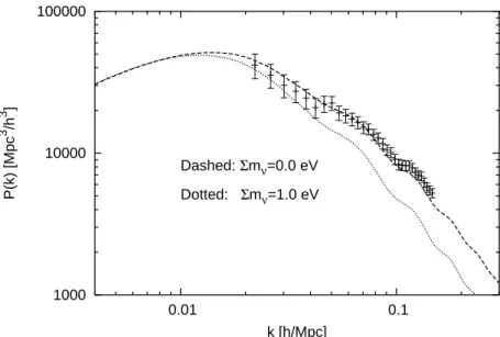
FIGURE 2. The large-scale matter power spectrum. The dashed line denotes the standardΛCDM model with zero neutrino mass; the dotted line has∑mν=1 eV. The data points are from the 2dF survey [16].
The physics of these anisotropies may be understood as follows. Before recombina- tion, photons and baryons form a tightly coupled fluid. This means that whenever gravity pulls the baryons into the dark matter potential wells and compresses the fluid, the pres- sure in the photons will push the fluid out again. This competition between gravity and pressure sets up acoustic oscillations, so that the compressed regions are hotter and the rarefied regions cooler. What we see in the CMB anisotropy spectrum are these acous- tic oscillations, just before recombination. After recombination, photons free-stream to infinity, preserving the oscillation pattern in their temperature. This makes the CMB anisotropies are very powerful probe of the baryon density, which determines to the sound speed of the baryon–photon fluid. Furthermore, since the CMB anisotropies can be thought of as a projection of the last scattering surface onto the sky, they also contain information about the geometry of the universe.
Probes of large-scale structure (LSS). The most powerful LSS probes at present are galaxy redshift surveys, with the Two Degree Field Galaxy Redshift Survey (2dFGRS) [14] and the Sloan Digital Sky Survey (SDSS) [15] being the largest to date. Essentially these surveys produce galaxy catalogues. With these catalogues one can calculate the galaxy number density at each point in space, and compute their two-point correlations,
hδ(~x+~r)δ(~x)i=
Z d3k
(2π)3jδkj2exp( i~k~r): (8) The quantity P(k)jδkj2is the power spectrum. In order to use this power spectrum to constrain cosmology, one makes one further assumption, that the clustering of galaxies traces that of the underlying matter distribution. In technical jargon, we say that the power spectrum reconstructed from galaxy clustering data, Pgal(k), is proportional to
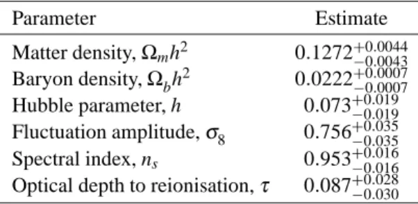
TABLE 1. Free parameters of the “vanilla” cos- mological model, their estimated values, and 68%
credible intervals from a combined WMAP+SDSS analysis [17, 18]. The fluctuation amplitude is ex- pressed in terms ofσ8, defined as the present-day rms fluctuations in a sphere of 8 h Mpc radius.
Parameter Estimate
Matter density,Ωmh2 0:1272+00:0044
:0043
Baryon density,Ωbh2 0:0222+00:0007
:0007
Hubble parameter, h 0:073+00:019
:019
Fluctuation amplitude,σ8 0:756+00:035
:035
Spectral index, ns 0:953+00:016
:016
Optical depth to reionisation,τ 0:087+00::028030
the underlying matter power spectrum Pm(k) up to a normalisation or bias factor, i.e., Pgal=b2Pm(k). This assumption should work well on large scales (i.e., small values of k), but is expected to fail on small scales. Where exactly it fails and how to correct for it is a major research question.
Other probes of LSS include weak gravitational lensing, Lyman-α absorption lines, cluster abundance, etc.. However, they all in one way or another rely on nonlinear modelling, which is presently not very well understood. I shall not discuss them here.
Figure 2 shows the LSS power spectrum. It is quite featureless, except for a marked turning point. Inflation generally predicts an initial power spectrum that is power-law like. The present day power spectrum ends up with a turning point because of evolution of the density perturbations: as the universe expands, perturbations with increasing wavelengths, or decreasing k values, “enter” the Hubble radius H 1, i.e., the wavelength becomes shorter than H 1 and the mode is in causal contact. The shortest wavelengths enter the Hubble radius during radiation domination; the perturbations in these modes therefore cannot grow. On the other hand, the larger wavelengths enter the Hubble radius late, during matter domination. These modes can grow. The net result is a suppression of the power spectrum at large k values, with a turning point at ktpcorresponding to the comoving Hubble radius during matter–radiation equality, ktpaeqHeq.
Cosmological model
The minimum model required to fit all current observational data has six free pa- rameters: the matter density Ωmh2 and baryon density Ωbh2 describe the energy con- tent of the universe; the Hubble parameter h gives the expansion rate; the initial con- ditions are specified by the initial power spectrum amplitude As and spectral index ns, such that Pini(k)=Askns; lastly, an astrophysical parameter τ, which affects only the CMB anisotropies, gives the optical depth to reionisation. The geometry of the model is flat, i.e., no spatial curvature. Furthermore, the initial conditions are adia- batic, meaning that the density perturbations in various components satisfy the relation δγ=4=δν=4=δm=3=δb=3. This relation is predicted by the simplest kind of inflation
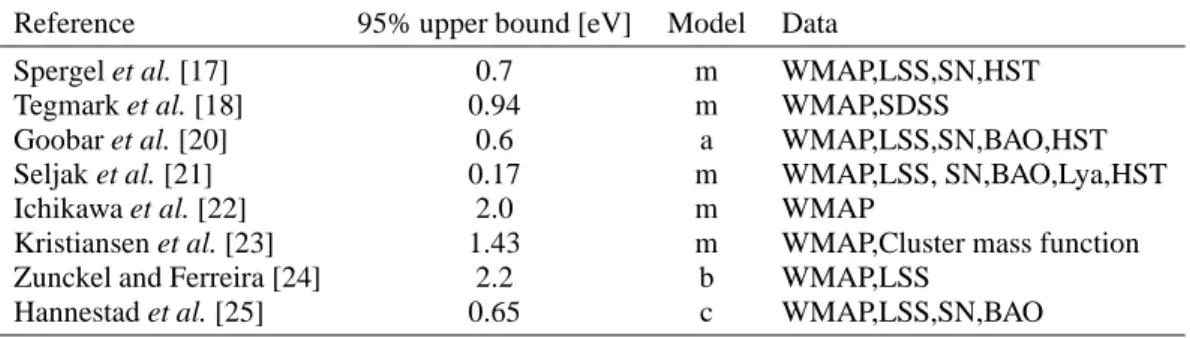
TABLE 2. 95% C.L. upper limit on the sum of neutrino masses∑mν from various cosmological observations. The acronym SN stands for supernova Ia, HST for Hubble Space Telescope key project, BAO for baryon acoustic oscillations, and Lya for Lyman-αabsorption lines. Two classes of models are considered: minimal models “m” with the six basic parameters of Table 1 plus neutrino mass, and extended models with additional free parameters to describe (a) dark energy beyond a cosmological constant, (b) non-adiabatic (isocurvature) initial conditions, and (c) the possible existence of axion hot dark matter.
Reference 95% upper bound [eV] Model Data
Spergel et al. [17] 0.7 m WMAP,LSS,SN,HST
Tegmark et al. [18] 0.94 m WMAP,SDSS
Goobar et al. [20] 0.6 a WMAP,LSS,SN,BAO,HST
Seljak et al. [21] 0.17 m WMAP,LSS, SN,BAO,Lya,HST
Ichikawa et al. [22] 2.0 m WMAP
Kristiansen et al. [23] 1.43 m WMAP,Cluster mass function
Zunckel and Ferreira [24] 2.2 b WMAP,LSS
Hannestad et al. [25] 0.65 c WMAP,LSS,SN,BAO
models, single-field inflation. Table 1 shows the current estimates of these parameters from the CMB experiment WMAP [17] and the SDSS galaxy redshift survey [18].
Of course, these six parameters are not the only ones that can affect cosmology: there are many more. These parameters are not included in most analyses at the moment be- cause they do not change significantly the goodness-of-fit. If we quantify the goodness- of-fit with the best fitχ2of the model, then it turns out that adding any one extra param- eter does not improve the best fitχ2by more than 3 or 4. This improvement is deemed too modest by many practitioners to justify the inclusion of extra parameters, although it is unclear where one should draw the line. Indeed, some of these extra parameters are physically extremely well motivated. Here I discuss the case of neutrino masses.
Constraints on neutrino masses
The idea of “weighing neutrinos” with cosmology [19], especially with LSS probes, hinges on an effect known as free-streaming. Neutrinos with sub-eV to eV masses contribute to the dark matter content of the universe: the heavier they are, the more their contribution. However, unlike ordinary cold dark matter, neutrinos are born with a high velocity, and become nonrelativistic only at very late times during structure formation.
While relativistic, their high velocity makes them difficult to capture into the dark matter potential wells, especially the ones that are narrow in width. This free-streaming inhibits the growth of the density perturbations on length scales below the free-streaming scale.
In the power spectrum, the presence of neutrino mass is manifested in a suppression of power on small scales. Figure 2 shows this suppression for a 1 eV neutrino.
Using this effect many authors have placed bounds on the sum of the neutrino masses.
Table 2 shows a selection of recent results. Clearly, the mass bound depends very much on which data sets are used to produce it. In particular, one can obtain an extremely tight bound of∑mν <0:17 eV if Lyman-α absorption lines are included. However, the Lya data used in [21] suffer from unknown systematic effects, and show a 2σ discrepancy
in the fluctuation amplitude when compared with CMB data. This discrepancy pushes the allowed parameter space to a “compromise region” and artificially pushes down the neutrino mass bound. Therefore, one should treat bounds from Lya with extreme caution.
Note also that the neutrino mass bounds are model-dependent: adding to the model parameters that are degenerate with the neutrino mass tends to relax the mass bound.
The bottom line is that precision cosmology can at present constrain the sum of the neutrino masses to order 1 eV. To obtain tighter bounds one would need to make assumptions about unknown factors such as the nature of dark energy and the initial conditions of the primordial density fluctuations.
FUTURE COSMOLOGICAL PROBES
Many cosmological probes have been planned for the next decade. There will be more CMB surveys, including the Planck satellite to be launched in 2008. Galaxy clustering surveys will probe LSS at higher redshifts, enabling us to track the evolution of structure and to probe the neutrino mass with greater sensitivity [26, 27, 28]. New kinds of ob- servations utilising different techniques to probe cosmology will also become available.
Here are some examples.
• Weak gravitational lensing of galaxies Light travelling from distant galaxies is bent by the foreground matter (both luminous and dark). This causes distortions (magnification and stretching) in the images of these galaxies. By measuring these distortions, one can reconstruct the foreground matter distribution (the lens) [29].
An interesting possibility is to bin the galaxy images by redshift, so that one can even obtain some 3D information about the foreground distribution. Using this technique, and together with future CMB observations, one can expect to probe the sum of the neutrino masses with a 1σ sensitivity of 0:01–0:05 eV [30, 31].
• Weak lensing of the CMB Light from the last scattering surface can also be lensed by the foreground matter [32]. Indeed, with the Planck satellite, one can hope to probe∑mν with sensitivity of 0:1 eV via CMB lensing [33, 34, 35].
• 21 cm These are emission lines from neutral Hydrogen spin flip at very high redshifts (z> 50). The density fluctuations in the primordial Hydrogen gas are imprinted on these emission lines. Thus, if detected they will offer a unique probe of the density perturbations in the “cosmic dark ages” [36]. However, detecting these emission lines require sophisticated radio telescopes, and currently planned facilities cannot look beyond z=20. Thus, 21 cm emission lines are for now better suited for the study of astrophysics, especially reionisation physics.
CONCLUSIONS
Cosmology offers an interesting way to probe many aspects of fundamental physics.
Neutrino properties are an excellent example. Using probes of the large-scale structure and of the cosmic microwave background anisotropies, we can already deduce that the sum of the neutrino masses must be less than about 1eV. This limit is already better than
those from laboratory experiments (roughly∑mν <6 eV [37, 38]). Future cosmological observations will do even better: in the most optimistic case, a sensitivity of σ(∑ν) 0:01 eV may be achievable in the next decade with CMB and weak gravitational lensing observations. With this kind of sensitivity, there is real hope that we may finally be able to measure the neutrino mass with precision cosmology.
ACKNOWLEDGMENTS
I would like to thank the organisers of the Carpathian Summer School of Physics for a most enjoyable meeting.
REFERENCES
1. J. Lesgourgues and S. Pastor, Phys. Rept. 429, 307 (2006) [arXiv:astro-ph/0603494].
2. S. Hannestad, Ann. Rev. Nucl. Part. Sci. 56, 137 (2006) [arXiv:hep-ph/0602058].
3. A. D. Dolgov, Phys. Rept. 370, 333 (2002) [arXiv:hep-ph/0202122].
4. S. S. Gershtein and Y. B. Zeldovich, JETP Lett. 4, 120 (1966).
5. R. Cowsik and J. McClelland, Phys. Rev. Lett. 29, 669 (1972).
6. G. F. Smoot et al., Astrophys. J. 396, L1 (1992).
7. C. L. Bennett et al., Astrophys. J. Suppl. 148, 1 (2003) [arXiv:astro-ph/0302207].
8. G. Hinshaw et al., Astrophys. J. Suppl. 170, 288 (2007) [arXiv:astro-ph/0603451].
9. L. Page et al., Astrophys. J. Suppl. 170, 335 (2007) [arXiv:astro-ph/0603450].
10. B. S. Mason et al., Astrophys. J. 591, 540 (2003) [arXiv:astro-ph/0205384].
11. K. Grainge et al., Mon. Not. Roy. Astron. Soc. 341, L23 (2003) [arXiv:astro-ph/0212495].
12. N. W. Halverson et al., Astrophys. J. 568, 38 (2002) [arXiv:astro-ph/0104489].
13. J. E. Ruhl et al., Astrophys. J. 599, 786 (2003) [arXiv:astro-ph/0212229].
14. M. Colless et al., arXiv:astro-ph/0306581.
15. J. K. Adelman-McCarthy et al., arXiv:0707.3413 [astro-ph].
16. S. Cole et al., Mon. Not. Roy. Astron. Soc. 362, 505 (2005) [arXiv:astro-ph/0501174].
17. D. N. Spergel et al., Astrophys. J. Suppl. 170, 377 (2007) [arXiv:astro-ph/0603449].
18. M. Tegmark et al., Phys. Rev. D 74, 123507 (2006) [arXiv:astro-ph/0608632].
19. W. Hu, D. J. Eisenstein and M. Tegmark, Phys. Rev. Lett. 80, 5255 (1998) [arXiv:astro-ph/9712057].
20. A. Goobar, S. Hannestad, E. Mortsell and H. Tu, JCAP 0606, 019 (2006) [arXiv:astro-ph/0602155].
21. U. Seljak, A. Slosar and P. McDonald, JCAP 0610, 014 (2006) [arXiv:astro-ph/0604335].
22. K. Ichikawa et al., Phys. Rev. D 71, 043001 (2005) [arXiv:astro-ph/0409768].
23. J. R. Kristiansen, O. Elgaroy and H. Dahle, Phys. Rev. D 75, 083510 (2007).
24. C. Zunckel and P. G. Ferreira, JCAP 0708, 004 (2007) [arXiv:astro-ph/0610597].
25. S. Hannestad et al., JCAP 0708, 015 (2007) [arXiv:0706.4198 [astro-ph]].
26. M. Takada, E. Komatsu and T. Futamase, Phys. Rev. D 73, 083520 (2006) [arXiv:astro-ph/0512374].
27. S. Hannestad and Y. Y. Y. Wong, JCAP 0707, 004 (2007) [arXiv:astro-ph/0703031].
28. F. B. Abdalla and S. Rawlings, arXiv:astro-ph/0702314.
29. M. Bartelmann and P. Schneider, Phys. Rept. 340, 291 (2001) [arXiv:astro-ph/9912508].
30. Y. S. Song and L. Knox, arXiv:astro-ph/0312175.
31. S. Hannestad, H. Tu and Y. Y. Y. Wong, JCAP 0606, 025 (2006) [arXiv:astro-ph/0603019].
32. A. Lewis and A. Challinor, Phys. Rept. 429, 1 (2006) [arXiv:astro-ph/0601594].
33. M. Kaplinghat, L. Knox and Y. S. Song, Phys. Rev. Lett. 91, 241301 (2003) [arXiv:astro-ph/0303344].
34. J. Lesgourgues et al., Phys. Rev. D 73, 045021 (2006) [arXiv:astro-ph/0511735].
35. L. Perotto et al., JCAP 0610, 013 (2006) [arXiv:astro-ph/0606227].
36. S. Furlanetto, S. P. Oh and F. Briggs, Phys. Rept. 433, 181 (2006) [arXiv:astro-ph/0608032].
37. V. M. Lobashev, Nucl. Phys. A 719, 153 (2003).
38. C. Kraus et al., Eur. Phys. J. C 40, 447 (2005) [arXiv: hep-ex/0412056].
![FIGURE 1. The cosmic microwave background temperature anisotropy spectrum for the standard ΛCDM model (see Table 1 for parameter values), with data from the WMAP satellite [8].](https://thumb-eu.123doks.com/thumbv2/1library_info/4007284.1540956/4.892.229.691.117.433/microwave-background-temperature-anisotropy-spectrum-standard-parameter-satellite.webp)