Approaches to identify groundwater discharge towards and within lowland surface water bodies on different scales

(1)

Approaches to identify groundwater discharge towards and within lowland surface water bodies on different

scales

Dissertation zur Erlangung des akademischen Grades Doktor rerum natuarlium

(Dr. rer. nat.) im Fach Geographie

eingereicht an der

Mathematisch – Naturwissenschaftlichen Fakultät Der Humboldt Universität zu Berlin

von

Dipl.-Geogr. Franziska Pöschke

Präsident der Humboldt-Universität zu Berlin Prof. Dr. Jan-Hendrik Olbertz

Dekan der Mathematisch-Naturwissenschaftlichen Fakultät Prof. Dr. Elmar Kulke

Gutachter 1: Prof. Dr. Gunnar Nützmann Gutachter 2: Prof. Dr. Tobias Krüger Gutachter 3: Prof. Dr. Stefan Krause

Tag der mündlichen Prüfung: 19. September 2016

(2)

(3)

Declaration of independent work

I declare that I have completed the thesis independently using only the aids and tools specified. I have not applied for a doctor’s degree in the doctoral subject elsewhere and do not hold ta corresponding doctor’s degree. I have taken due note of the Faculty of Mathematics and Natural Sciences PhD regulations, published in the Official Gazette of Humboldt-Universität zu Berlin no 126/2014 on 18/11/2014.

(4)

Acknowledgement

Most of all I would to thanks my supervisors Dr. Jörg Lewandowski and Prof. Dr. Gunnar Nützmann, who gave me the freedom of following my personal research interests. Thanks also to Prof. Dr. Peter Engesgaard for the support in groundwater modeling and the opportunity for working in his group in Copenhagen.

Many thanks also to Dr. Georigy Kirillin and Dr. Christof Engelhardt, who stirred up my enthusiasm for lake physics and gave me another perspective on groundwater – surface water interaction.

I also want to thank Uwe Kaboth, who had an invaluable knowledge about the local and regional hydrogeology of the federal state of Brandenburg.

Special thanks also to all the people who supported me during my field work: Christine Sturm, Jörg

Friedrich, Grit Siegert, Hauke Dämpfling, Adrian Brox, Sandra Bölck, Hendrik Schlichting, Bibiana Menosi, Hans-Jürgen Exner, Elke Zwirnmann, Gabriele Mohr and Michael Sachtleben.

I need to thank the whole team of the AQUALINK graduate school. They enabled me an insight into

different scientific fields and were a great support during my whole PhD time. Especially, I like to say thanks to Christian Lehr for his support in statistics and the great cooperation.

Furthermore, I need to thank all of my colleagues and friends for the support and fruitful discussions during the last years, namely Karin Meinikmann, Stefanie Burkert, Sebastian Rudnick and Andrea Sacher.

Last but not least I thank my family and friends, who always believed in me and helped me to find my way.

(5)

Abstract

Although the point sources of nutrient input into surface water were significantly reduced in the past decades, there is still an ongoing eutrophication in the lakes and rivers in the North-Eastern German Lowlands. This is mainly related to the diffuse entering pathways. One relevant pathway might be the groundwater. However, the characterization of subsurface flow and its interaction with the surface water in lowlands is difficult. The main reasons for that are the heterogeneously deposited unconsolidated rocks, in which complex and nested aquifer systems (local, intermediate, and regional) establish. Hence, groundwater discharge occurs on different scales, whereas each scale is dominated by different drivers.

The aim of the presented thesis is to apply different methods to determine the parts of lowland aquifer systems which contribute mass, substances and energy into specific surface waters. Therefore, two approaches were used (1) a hydrogeological and (II) a limnological/hydrological one.

The focus of the hydrogeological approach was set on the characterization of groundwater flow systems on different spatial scales. On a small scale (10² m) a principle component analysis was conducted on time series of water level measurements in a river and in the adjacent groundwater of the floodplain. According to different responses of the groundwater on surface water induced pressure waves, areas with different hydraulic connectivity were identified. For the same aquifer, the small scale nutrient (≤ 10¹m) distribution in the near-surface groundwater was also investigated. A close linkage between the nutrient distribution and the small-scale topography within the floodplain was detected. Both studies illustrate that comparatively “easy–to-measure” data in a high spatial and temporal resolution are sufficient for the detection of subsurface preferential flow paths as well as spots of potential nutrient sources. On a larger scale (10³ m) a study was conducted which investigated the impact of groundwater leakage on the characteristics of a local flow system. Therefore, a simple 2D numerical groundwater model (steady state) was set up for the subsurface catchment of a lake. The model could illustrate that leakage lead to a decrease of the amount of groundwater, which enters the lake and, an increase of the length of the groundwater flow paths. Hence, groundwater leakage needs to be considered for the determination of local groundwater flow systems.

The limnological approach based on the hypothesis that physical and chemical differences between groundwater and lake water can be used to identify areas, where groundwater is exfiltrating. The presented studies tested if it is possible to use temperature measurements at the lake surface (thermal infrared imaging and in situ measurements) in spring, when the warmer groundwater is floating on the colder lake water. However, the comparison of the temperature measurements with hydrogeological and lake data, indicate that in the present case the observed temperature pattern are the result of lake internal processes. However, the aerial detection of groundwater spots should be possible at least for lakes with small volumes and intense groundwater discharge.

(6)

Zusammenfassung

Der Eutrophierungsprozess schreitet in vielen Oberflächengewässern im Norddeutschen Tiefland weiter voran, obwohl die punktuellen Quellen des externen Nährstoffeintrags in die Gewässer zum Großteil beseitigt wurden. Der Grund dafür ist der Eintrag aus diffusen Quellen, wie zum Beispiel dem Grundwasser. Die unterirdischen Fließsysteme und deren Interaktion mit den Vorflutern sind jedoch sehr schwer zu quantifizieren. Dies liegt vor allem an der räumlichen Heterogenität der abgelagerten Lockergesteine, in denen sich hydraulisch komplexe Aquifersysteme ausbilden. Der Grundwasserabfluss findet somit auf verschiedenen Skalen statt, wobei auf jeder Skala andere Steuerungsgrößen wirken.

Ziel der vorliegenden Arbeit ist es mittels verschiedener Ansätze die Bereiche in einem Tieflandsaquifer zu ermitteln, die zum Massen-, Stoff- und Energieeintrag in Oberflächengewässer beitragen. Dazu wurden zwei Herangehensweisen gewählt: (I) die hydrogeologische und (II) die limnologische/ hydrologische.

Der Schwerpunkt der Ersteren liegt auf der Charakterisierung der unterirdischen Fließsysteme auf verschiedenen räumlichen Ebenen. Auf kleinskaliger Ebene (<10³ m) wurde mittels einer Hauptkomponentenanalyse von Zeitreihen von Grundwasser- und Oberflächenwasserständen diejenigen Bereiche eines Auenaquifers ermittelt, die eine besonders hohe hydraulische Konnektivität zum Vorfluter haben. Im selben Aquifer wurde auch das kleinskalige Vorkommen (≤

10¹ m) der Nährstoffe im oberflächennahen Grundwasser untersucht. Hier wurde ein enger Zusammenhang zwischen kleinskaliger Topographie und der Nährstoffverteilung nachgewiesen. Beide Arbeiten zeigen, dass mit Hilfe

vergleichsweiser einfacher Datengrundlagen präferentielle unterirdische Fließwege sowie die Lage potentieller Nährstoffquellen abgeschätzt werden können. Grundlage dafür ist eine hohe räumliche und zeitliche Auflösung der Daten. Auf großskaliger Ebene (>10³ m) wurde eine Studie durchgeführt, die die Interaktion zwischen lokalem und regionalem Grundwasserfluss und deren Einfluss auf die Hydrologie eines tiefen, nährstoffarmen Sees untersucht. Dies erfolgte mittels eines nummerischen 2D Grundwassermodells (steady state) für das Grundwassereinzugsgebiet des Sees.

Das Modell zeigt folgende Effekte der Tiefenversickerung auf das Grundwasserfließgeschehen im lokalen Fließsystem:

Die Menge an Grundwasser, welche in den See entwässert verringert sich. Außerdem erzeugt der in die Tiefe gerichtete Gradient eine Verlängerung der unterirdischen Fließpfade. Somit konnte die Studie zeigen, dass bei Ermittlung des Grundwassereintrags in einen Vorfluter Tiefenversickerung berücksichtigt werden sollte.

Die limnologische Herangehensweise baut auf der Hypothese auf, dass physikalische und chemische Unterschiede zwischen Grund- und Oberflächenwasser genutzt werden können, um die Bereiche, in denen Grundwasserexfiltration in einem See stattfindet, zu identifizieren. In der vorliegenden Arbeit wurde getestet, ob dies an Hand von

Temperaturmessungen an der Seeoberflächen (thermische Infrarotaufnahmen und in situ Messungen) möglich ist. Dafür wurden Messungen im Frühjahr nach der Vollzirkulation in zwei aufeinander folgenden Jahren durchgeführt. Der Vergleich der Oberflächenwassertemperaturen mit hydrogeologischen Daten und zusätzlichen Informationen zu seeinternen Prozessen zeigte jedoch für die zwei untersuchten Seen, dass bei seeinternen Prozesse die

Temperaturverteilung an der Seeoberfläche dominieren. Es ist allerdings nicht auszuschließen, dass diese Methode zur Detektion von Grundwasserzustrom an Seen mit anderen Randbedingungen (kleineres Seevolumen, größerer

Grundwasserzustrom) funktioniert.

(7)

Figures

Figure 1.1-1: Concept of volume and velocity properties of groundwater and surface water and its relation to the spatial and temporal dimension. The red line represents the properties of the interface...16 Figure 2.1-1: Location of the North-Eastern German Lowlands and subdivision into the different kind of landscapes and hydrological regimes of the Saalian and Weichselian ice ages...22 Figure 2.1-2: Position of the three study sites within in the North-Eastern German Lowlands (A). Subsurface catchment of the upper aquifer and the interpolated contour lines for groundwater heads for Lake Arendsee (B), Lake Stechlin (C) and the investigated oxbow of the river Spree (D). The groundwater data from Lake Arendsee ground on Meinikmann et al. (2013). The determination of the groundwater catchment and contour lines for Lake Stechlin are based on available data from the Landesamt für Umwelt, Gesundheit und

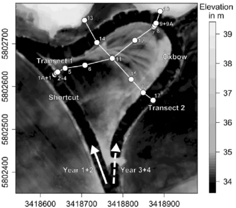
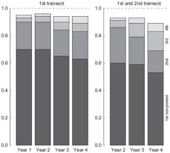
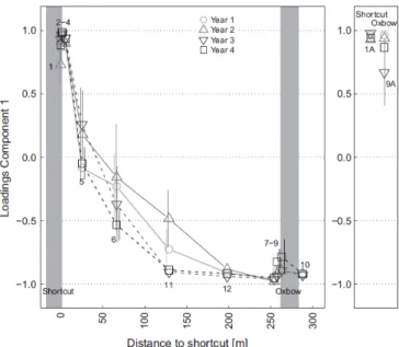
Verbraucherschutz (LUGV) Brandenburg (2012). The groundwater contour lines for the River Spree were made available from the LUGV (2012). The data from Lake Arendsee are projected in WGS 84 UTM 32N and in WGS 84 UTM 33N for Lake Stechlin and the oxbow of the river Spree...24 Figure 2.1-3: Interpolation of the average annual catchment according to the findings of Holzbecher (2001) for three years with different precipitation condition: dry (2003); average (1973) and wet (1983)...25 Figure 3.2-1: Elevation map based on a LIDAR-Scan from 3rd December 2009 with 1 m grid size and 0.3 m resolution for altitude in projection ETRS89 UTM Zone 33. First transect of groundwater observation wells in west-northeast direction and second transect in northwest-southeast direction. At both ends of the first transect there was a water level gauge situated in the stream (1A + 9A). The filled arrow marks the main stream flow in the first two years of the study, the dashed arrow the main stream flow in the third and fourth year. The flow through the other reach was blocked in both situations...37 Figure 3.2-2: Ratio of overall variance explained by the first four principle components of the PCA of the data set of the first transect (left) and of the PCA of the joint data set from both transects (right)...42 Figure 3.2-3: Loadings of groundwater observation wells of the first transect on the first principle component vs. distance to shortcut (left) and of the stream water gauges (right). Mean of loadings of the 4 quartiles of the hydrologic year (Oct.-Sept.) and their corresponding confidence intervals. Only confidence intervals >

0.2 are shown. On the left panel the grey bars indicate the position of the stream...43 Figure 3.2-4: Loadings of the groundwater observation wells of the first principle component of the second transect vs. distance to the northern end of the transect two at observation well 13 (left) and of the stream water gauges (right). Mean of loadings of the 4 quartiles of the hydrologic year (Oct. – Sept.) and their corresponding confidence intervals. Only confidence intervals > 0.2 are shown. On the left panel the grey bars indicate the position of the river...43

(11)

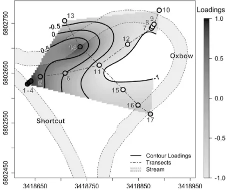
Figure 3.2-5: Spatial interpolation of loadings of the first component based on the mean of the loadings of the 4 quartiles of the third observation year (Oct. – Sept.). Projection is in ETRS89 UTM Zone 33. Values <

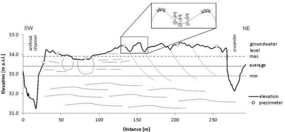
-1 are artefacts and excluded...44 Figure 3.3-1: Conceptual model of the study site visualizing topography (scalable) and subsurface

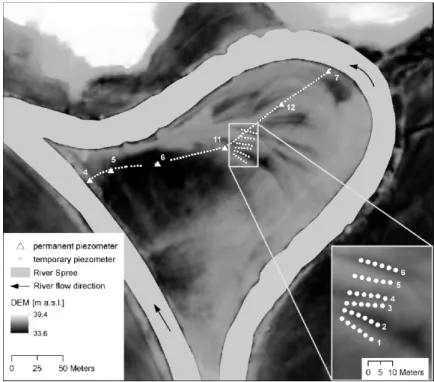
stratification of the floodplain (not to scale). As a result, microhabitats with different plant communities have formed (modified from Lewandowski et al., 2009)...52 Figure 3.3-2: Digital elevation model (DEM) of the island and position of the temporary and permanent piezometers; multi-level sampler (sampled in April 2009, August and October 2011) are located at the same positions as the permanent piezometers. The first horizontal campaign of the temporary piezometers along the transect of permanent piezometers were sampled in October and November 2008. The second horizontal campaign on the ridge and swale structure was conducted in July 2010...53 Figure 3.3-3: Validation of GPR profiles by drill log cores. The core profiles illustrate the main grain size of the soil horizon (H = peat; u = silt; fS = fine sand; mS = medium sand). In the GPR profiles, coarser grain sizes are colored from yellow to violet (sand and gravel fraction). Silt and peat are colored white to light grey. Silt and peat can be distinguished by the layers below: Below peat layers, sediment stratification is visible whereas below silt and clay is not. The pictures illustrate a 2 m wide GPR profile, and the black bordered boxes show the position of the cores. The location of the GPR profiles is shown in Figure 3.3-4.. .58 Figure 3.3-4: Results of the GPR survey. Figure (A) illustrates the position of the GPR profiles, which are shown in (B). The red points are located at the positions of changing stratification of the fluvial sediments.

(C) and (D) show the GPR profile along the transect of permanent piezometers. Because of the length of the profile it was cut into (C) and (D). Three fundamentally different stratification types of the floodplain can be distinguished. Beside the previously mentioned changes of stratification of the fluvial sediments, the third type can be found in depths below 4 m, which are glacifluvial sediments...59 Figure 3.3-5: Median (n = 5) concentration depth profiles of dissolved phosphate, ammonium, and dissolved iron and their location along the transect of permanent piezometers. The dashed line shows the border between the identified upper layer, which is influenced by water level fluctuations and the lower layer, which is not...61 Figure 3.3-6: Concentration patterns determined by the linear investigation with temporary piezometers (first campaign) along the transect of permanent piezometers. Zone marked in grey illustrates locations of

temporary piezometers in the second campaign (Figure 3.3-8). Zones I - IV have been identified as

stratigraphically different zones based on DEM and GPR...63

(12)

Figure 3.3-7: Concentration distribution of phosphate, ammonium, and dissolved iron for the four sections.

The differences are significant between the SRP concentrations of section I–III, II–IV and III–IV. NH4+

differences are only significant between Sections II–III and Fe2+ between I–III and III–IV...64 Figure 3.3-8: Results of the investigation of groundwater below ridges and swales with temporary

piezometers (second campaign). Panels A–D show the average (n = 6) for each ridge (n = 3) or swale (n = 3), respectively (compare locations shown in Figure 3.3-2). Panels E–G show the boxplots for the trend adjusted data. The differences between ridges and swales are significant for phosphate and ammonium, whereas there is no significance for dissolved iron...65 Figure 3.4-1: Concept of nested flow systems and layered aquifer systems in low land areas. The focus of the present study is set on the local flow systems in recharge areas in the head areas of low land landscapes...73 Figure 3.4-2: The left side illustrates the location of the study site within Germany (red dot).The right side gives an over view of the elevation groundwater catchment and bathymetry of Lake Stechlin. The black dots mark the position of the groundwater wells used for the conceptual model and the numerical simulation...75 Figure 3.4-3: Water level of Lake Stechlin and five groundwater wells from November 1957 to October 2012. The wells P37, P03, P02 and P40 are filtered in the upper unconfined aquifer. Well P01 is filtered below a glacial till layer. For the location of the wells compare Figure 3.4-2...78 Figure 3.4-4: Groundwater levels that would establish along a flow path from the catchment to the lake for a fixed lake head of 59.6 m a.s.l., a groundwater recharge of 100 mm a-1 and different hydraulic conductivities (kf). Measured average groundwater levels (1962 – 1999) are shown and compared to groundwater levels calculated based on equation 1 assuming steady state conditions. The figure illustrates that the system is very sensitive to small changes in hydraulic conductivities...79 Figure 3.4-5: Conceptual Model for the groundwater flow towards Lake Stechlin and the deeper aquifers.

The grey box indicates the area where is an expected change between groundwater level fluctuations. The groundwater level close to the lake is impacted by the lake level fluctuations; the groundwater on the left side is not...80 Figure 3.4-6: 2D vertical cross-sectional FEFLOW model for a groundwater transect at Lake Stechlin. The dark grey area indicates the area used for the numerical simulation; the white grey area is the total extension of the system, which shows also the thick unsaturated zone. The black points show the position of the observation points. The lake water level was used as fixed head boundary condition (blue line) of 59.60 m a.s.l., the average groundwater recharge (100 mm a-1) was applied at the top of the model domain (orange line). At the bottom there were different groundwater leakage areas, which were used in different model scenarios: the leakage area 1 (black), 2 (red) and 3 (dark grey). Please note the different horizontal and vertical scales...82

(13)

Figure 3.4-7: Flow paths and distribution of Darcy flow velocities for simulation I b, I c, and II. The red line shows the area water is leaking into the deeper aquifers...85 Figure 3.5-1: Thermal infrared image of Lake Arendsee taken on 22March 2012. Groundwater entering the lake in near-shore zones in the south of the lake floats as thin warm layer on top of the water body and spreads out onto open waters. Water table contour lines in the catchment of Lake Arendsee and delimitation of the catchment were determined based on 32 groundwater observation wells. Size of near-shore circles indicates rates of groundwater discharge in that shore section based on sediment temperature depth profiles (Schmidt et al., 2006) taken at the end of July and the beginning of August 2012. Blue triangles indicate location of the 4 small ditches entering the lake and the numbers in parentheses indicate the percentage of the overall surface water inflow entering the lake via that ditch in March 2011 (no measurements conducted in March 2012)...95 Figure 3.5-2: Water temperatures (TWater) of Lake Arendsee in 1.5 m water depth and weather conditions over Lake Arendsee (air temperature TAir, wind velocity and radiation) in March 2012. Vertical dashed lines designate the date of the TIR survey...97 Figure 3.5-3 : The groundwater floating criterion G (Equation 3.5-10) in Lake Arendsee in March 2012. u* is the friction velocity at the lake surface, w* is the convective velocity scale, and Ri is the Richardson number.

The gaps correspond to the periods of negative G, when no groundwater floating is possible independent of the absolute value of G...100 Figure 3.6-1: Location of study sites, positions of lateral temperature measurements (black circles) and thermistor chains (black triangle). The data are projected in UTM 32 WGS 84 for Lake Arendsee and UTM 33 WGS 84 for Lake Stechlin, respectively...109 Figure 3.6-2: Set up for the in-situ horizontal temperature investigation. Floating material was fixed at the end of the data logger to ensure that the temperature sensor is placed one centimeter below the water surface (scale on the right picture is in cm)...110 Figure 3.6-3: Comparison of interpolated temperatures of sensors floating on the lake surface (left column) and the TIR image (right column) on 24 April 2013. Images were taken for Lake Arendsee at 8:16 - 8:21 h (upper row) and for Lake Stechlin at 9:06 - 9:15 h (lower row). The data are projected in UTM 32 (WGS 84) for Lake Arendsee and UTM 33 (WGS 84) for Lake Stechlin, respectively. The figure illustrates the

deviation of the temperature from a spatial mean during the time of flight, which is written in the right lower corner of each panel...115 Figure 3.6-4: Daily pattern of the surface temperatures of Lake Arendsee (left columns) and Lake Stechlin (right columns) from 23 to 30 April 2013. The figures are interpolated from the deviations of the spatially averaged temperatures of each day. The daily average temperature is written in the right corner of each single

(14)

image. Additionally, the average wind direction and wind speed are shown as an arrow in the upper left. Note that the figure shows the local deviations of the daily mean of the entire lake surface...117 Figure 3.6-5: Upper 12.5 m of CTD-profiles in Lake Arendsee taken on 28 April 2013 between 18:00 and 19:30 h. (a) Transects from the southern to the eastern shore (T1 - T6), (b) from the southern to the northern shore (T7 - T12), and (c) location of transects in the lake and lake surface temperatures calculated based on loggers A01 to A12. The figures (a) and (b) indicate an upwelling of metalimnic water...119 Figure 3.6-6: The Lake number (LN), the Wedderburn number (W) and the Schmidt Stability (S) in (A) Lake Arendsee and (B) Lake Stechlin. The Schmidt stability is scaled with the mean density 0 and the mean lake depth H, providing a direct estimate of the internal wave speed (see the text for further explanations). Dark gray area with a thick vertical line demarcates the preceding winter stratification and the overturn. The light gray area marks the period of the surface temperature observations. The overturn periods are designated by values S ≤ 0 seen at the logarithmic plot as ‘no value’ gaps...120 Figure 4.3-1: Time series of the Lake Number (Ln), Wedderburn Number (Wd) and Schmidt Stability (St) of Lake Arendsee in 2012 (left) and 2013 (right). The red line marks the threshold for L and W for upwelling.

...131 Figure 4.3-2: Temperature time series of different depth in the lake bed sediment of Lake Stechlin. Depth profiles were measured in 2 m distance from the shore...132

(15)

Tables

Table 1.1-1: Examples for characteristic physical, chemical and biological properties of groundwater and surface water bodies in temperate regions...17 Table 2.1-1: Long-term average of precipitation and temperature from 1981-2010 for weather stations close to the study sites (data source: Deutscher Wetterdienst, 2014)...23 Table 3.3-1: Sediment and topographical characteristics of the four different zones within the floodplain....58 Table 3.3-2: Results of the Mann–Whitney U tests between the upper and lower layers of the MLS

investigations. W is the test statistic, p the probability and r the magnitude of the effect size. Statistically significant differences between the upper and the lower layers are colored in grey...64 Table 3.3-3: Spearman’s correlation coefficients for concentration of soluble reactive phosphate, ammonium, and dissolved iron for the temporary piezometer located in the swales and on the ridges (second campaign).

(* p < 0.001; ** p < 0.01)...66 Table 3.4-1: Water levels at 05/12/2014 of the deep well Hy Ngw 1/2010 at filtered at different depth. The well is situated close to the wells P01 and P40 (compare Figure 3.4-2)...77 Table 3.4-2: Cross-correlations of the water levels and time lags (month) of selected wells and the lake...78 Table 3.4-3: Overview over the eight simulation scenarios which consider different hydraulic conductivities and different leakage areas. The leakage fluxes listed in the table are the fluxes which produced the best fit between observed and simulated groundwater levels...82 Table 3.4-4: Results of the eight different model scenarios. Positive deviations between simulated and measured groundwater levels indicate an overestimation while negative values indicate an underestimation.

Furthermore, the Root Mean Square Error is shown to compare the performance of the different model runs.

The budget columns show the volume of water entering the lake or the deeper aquifers...83 Table 3.4-5: Comparison of observed and simulated groundwater exfiltration at the near-shore areas...84 Table 3.6-1: Characterization of Lake Arendsee and Lake Stechlin...108

(16)

1. Introduction

1.1 Groundwater discharge towards and within surface water bodies

In the past decades the ongoing eutrophication of surface water bodies in the North German Lowlands became an issue in public and science (e.g. LUGV, 2009; Hupfer and Nixdorf, 2011). After the reduction of point sources the diffusive entry pathway got the major role in nutrient import into lakes and rivers (e.g. Schindler, 2006). Beside diffuse imports via re-suspension from the sediment or atmospheric deposition (Schwoerbel and Brenelberger, 2005), groundwater can act as major source for dissolved substances like nutrients (e.g. Meinikmann, 2015). This fact points to a high connectivity between both water bodies. In lowland areas the connection is given by high permeable sediments forming large and thick aquifers where the surface waters are embedded. However, the physical, chemical and biological properties of groundwater and surface water differ a lot (Table 1.1-1), which is the main reason for investigating both water bodies separately in the past and the little knowledge about the consequences of the tide connection between both water bodies.

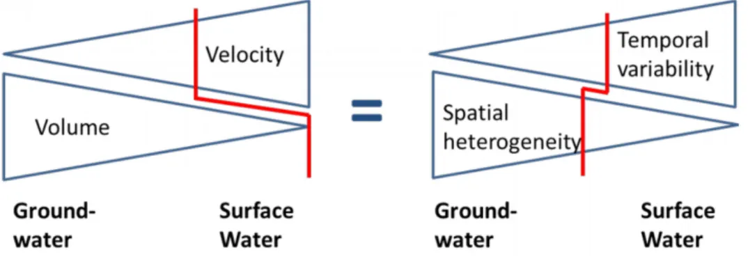
Figure 1.1-1: Concept of volume and velocity properties of groundwater and surface water and its relation to the spatial and temporal dimension. The red line represents the properties of the interface.

To understand the processes occurring in both systems requires knowledge about their spatial and temporal scales (Figure 1.1-1). The spatial extension of the groundwater is much larger in comparison to the surface waters. Beside the overall hydraulic gradient, the groundwater flow is determined by the sediment. Since this is not evenly distributed there is a large spatial heterogeneity of groundwater flow within an aquifer. For instance, SkØien and Blöschl (2003) analyzed the groundwater level fluctuations of 3539 wells for Austria and found that the relationship is limited to 7 km. Furthermore, the

sediments cause a slowdown of the groundwater flow velocity. This also implies that the reaction on

(17)

short term temporal fluctuations is small and dampened in comparison to the meteorological input.

The surface waters behave in the opposite way. The spatial heterogeneity is smaller and also easier to determine as for aquifer systems whereas the short-term temporal variability is increased due to the direct reaction of meteorological forces like precipitation, snow melt or wind.

Table 1.1-1: Examples for characteristic physical, chemical and biological properties of groundwater and surface water bodies in temperate regions

Groundwater Surface water

river lake

Physical properties

general flow characteristics laminar turbulent turbulent

flow velocity scale [m s^-1] ≤ 10^-3 1 - 10¹ 10^-1

average residence times large small medium

temperature constant seasonal

variability

Epilimnion: seasonal variability Hypolimnion:

constant

Chemical properties

redox conditions Decreasing

oxygen with depths

oxygenated Oxygenated during mixis, decreasing oxygen with depth during stratification

Biological properties

dominant trophy heterotrophic autotrophic &

heterotrophic

autotrophic &

heterotrophic

metabolism decreased due to

low temperature, no light and less

organic matter

high, depending on the water temperature

high, depending on the water temperature and oxygen saturation

(18)

Since both systems are different in characteristics and behavior they share an interface, which is characterized by sharp biogeochemical and physical gradients. So even if this interface is comparably small (Figure 1.1-1), the flow and processes such as microbial turnover, storage and release of substances are faster than in the adjacent groundwater. This lead to an increased interest in science during the past decades (e.g. Winter, 1995; Woessner, 2000; Fleckenstein et al., 2010; Wondzell, 2015). The results can be summarized as follows:

(1) The exchange between groundwater and surfaces water does not occur over the whole interface and is further concentrated in specific areas (spatial heterogeneity) (McBride and Pfannkuch, 1975; Krause et al., 2014).

(2) Even if a specific area is known, there are temporal variations according to the season and the general weather situation (Winter, 2005).

(3) The significance of the impact also depends on the size and the volume of the surface water and the adjacent groundwater body (Rosenberry et al., 2015).

(4) The anthropogenic manipulation of surface waters superimposes the complex natural conditions (Winter et al., 1999; Gessner et al., 2014).

As all four dimensions are highly dynamic, recent research focused on smaller spatial and temporal scales to understand the detailed processes occurring at the interface (Fleckenstein et al., 2010).

Hence, there is basic knowledge about small to medium scale flow pattern within the interface but there are fewer answers on the following questions:

1. Where does the groundwater entering the interface come from? So it needs to be clarified in which way different source areas contribute to the groundwater exfiltration into surface waters.

2. When the water has passed the interface, where does it go and what kind of effects does it have on the surface water?

Answers to these questions would improve management measures or definition of protection areas.

The question concerning the source of the groundwater is of special interest for lowland areas, as bigger a catchment results in a larger possibility of entering pathways. Tóth (1963) illustrated that there is a layered system within unconfined aquifers. He described a nested gravity driven

groundwater flow system, which is controlled by the topography of the water table and the sediment.

He also identified three main flow systems: local, intermediate and regional. Winter (1983) could further illustrate that these flow systems are not constant in time and space. Their spatial extension

(19)

mainly depend on the recharge conditions and, therefore, on climatic factors. These findings imply that water recharging the groundwater within a specific catchment does not necessarily discharge into the closest surface water. Assuming that there is a decreasing anthropogenic impact from local to regional flow systems, the water supply from deeper flow systems would be able to buffer the import of substances by dilution (Falkenmark and Allard, 1991). However, the determination of the origin of the exfiltrating groundwater is still a challenge. Nowadays it is possible to distinguish clearly between infiltrated surface water and “real” groundwater close to the shoreline e.g. by measuring the stable isotopes relation of δO¹⁸ and deuterium (Dincer, 1968; Krabbenhoft et al., 1994; Hofmann et al. 2008).

This allows the clear identification of exfiltration areas of groundwater into the surface water and the infiltration areas of surface water into the aquifer. However, using natural tracers like stable isotopes always requires a significant difference between the observed compartments to distinguish the flow path (Käss, 2004), which is difficult to determine in a single hydrological compartment by simple field investigation. In most cases, flow systems were determined by multi-factorial analysis (e.g. Menció et al. 2012) and by numerical groundwater modeling mostly in combination with chemical transport modeling (e.g. Blair et al., 1991; Frapporti et al, 1995; Hunt et al., 2001; Frind et al., 2002). The second approach allows the evaluation of different driving and controlling variables of the system, like the hydraulic conductivity, anisotropy and groundwater recharge. Nevertheless, there are still large uncertainties according to choice of the right variable or variable combination to explain a measured parameter (Frapporti et al., 1995). Furthermore, also models are related to a specific spatial scale and temporal resolution depending on the available input data and the computational effort (Blöschl, 2011).

Beside the determination of the size of the local system and the loadings in this part of the aquifer, knowledge about the groundwater flow paths is required. These are mainly determined by the sediments within an aquifer (e.g. Freeze and Cherry, 1979; Hölting and Coldewey, 2009). Already small variations in the grain size composition lead to significant differences in groundwater flow, due to higher and lower hydraulic resistances. This is especially a challenge for areas connected to surface waters, like riverine floodplains. Since these parts of the aquifer were formed by the river activity itself it is characterized by its patchiness (e.g. Bridge, 2003). Hence, the characterization of the sediment distributions in these areas is still a challenge. Classical methods like drill logging deliver high resolved information at the point scale, but are coarse at the spatial scale. Geophysical

approaches cover larger areas, but on the other hand they are cost-intensive, sometimes difficult to interpret and difficult to handle in hardly accessible areas.

The second question is dealing with the detection of groundwater within the surface water and the groundwater impact on it. From marine settings it is known, that exfiltration areas can be detected by temperature and conductivity measurements. This is based on the fact that the density of the marine

(20)

waters is higher due to the salinity and the groundwater is floating on the top of the surface water (e.g.

Danielescu et al. 2009, Peterson et al., 2009, Garcia-Solsona et al., 2010). For freshwater systems it is assumed that the detection depends on the type of surface water. Due to the highly turbulent character of streams and rivers, the entering groundwater is mixed immediately with the surface water.

However, a heat signal of the groundwater is still detectable if the stream is small and the groundwater discharge is large enough (Torgersen et al., 2001; Schuetz and Weiler, 2011). This is different for lakes. Depending on the thermal cycle of the lake, inflowing water will float in a specific layer (Peeters and Kipfer, 2009), e.g. for groundwater this can be shown by measuring radon concentrations along a vertical depth profile (Kluge et al., 2007). Radon concentration is a natural tracer for

groundwater. Its half-life is about 3.8 days and in the surface water there is little production of radon.

Additionally, as soon radon-rich water gets in contact with air it outgases into the atmosphere.

Therefore, surface waters contain only small radon concentration in comparison to groundwater. The study of Kluge et al. (2007) could show that there was an enrichment of radon concentration in the thermocline, which was related to discharging groundwater. So if it is possible to detect the areas of groundwater exfiltration within a surface water body it would also narrow the source areas of the entering groundwater (Lewandowski et al. 2013, study IV).

(21)

1.2 Research objectives and hypothesis

The overall aim of the present thesis is to contribute to the general understanding of the dynamics of groundwater – surface water interactions in temperate low land areas. The focus was set on the

determination of subsurface areas exfiltrating into specific surface water and the detection of the areas, where groundwater exfiltration occurs in the surface water. Therefore, two different approaches were used: (I) The hydrogeological and (II) The limnological/ hydrological approach.

The hydrogeological approach aimed in (1) the identification of subsurface flow paths towards rivers and lakes and, (2) the determination of the extension of groundwater flow systems contributing to surface water. Therefore, it is necessary to consider the scale dependent control parameters of groundwater flow. On small scale (≤ 10³ m) controlling parameters are sediment, topography, vegetation and water stage fluctuations of the river. For instance, in floodplains the parameters are spatially heterogeneous distributed due to fluvio-geomorphodynamics. As a result of the patchiness, floodplains are highly effective concerning nutrient retention, turnover and transport. However, it is still a challenge to identify the parameter distribution in a sufficient good resolution, e.g. to detect areas with higher or poorer hydraulic connection to surface water.

Hypothesis (1) assumes a linkage between small-scale parameters impacting groundwater flow and nutrient distribution within lowland floodplains. If this is the case, it would be sufficient to capture one parameter to get a rough idea of subsurface flow paths and potential sources for nutrients.

With increasing scale (>> 10³ m) the position of the surface water within a landscape decides about the size of the subsurface catchment (Tóth, 1963, Winter et al., 2003); the topographically lower a surface water is situated, the more complex is the groundwater flow towards those water bodies. Hence, lakes and rivers in head areas - where groundwater recharge occur - receive water only from local

groundwater catchment, which extension can be determined easily. However, groundwater leakage into deeper aquifers is present in head waters, which should affect the extension of the local flow system.

Hypothesis (2) says that groundwater leakage into deeper aquifers needs to be considered for the determination of local groundwater flow systems of a lake in lowland head waters.

The limnological/ hydrological objective aims in determining areas where groundwater exfiltrates into surface water. Therefore, it is assumed, that there are different physical and chemical properties of groundwater and surface water which can be used as tracer. In the present thesis temperature was used.

(22)

Hypothesis (3) assumed that groundwater of a constant temperature of 10 °C will float on the surface of a lake, when: (a) The lake starts to stratify after spring overturn and has surface temperatures of

>4 °C and < 10 °C. (b) There is no wind and (c) The heat flux is from the atmosphere to the surface water body (air temperature > lake temperature). Airborne methods such as thermal infrared imaging can be used for detection.

2. Material and Methods

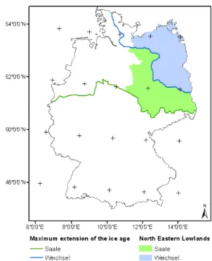
2.1 North Eastern German Lowlands The North Eastern Lowlands of Germany were formed during the past ice ages; the Saalian ice age (~130.000 years before present) dominates the southern and the western part, whereas the Weichselian ice age (~10.000 years before present) formed the northern and the eastern part (Figure 2.1-1). The glacial deposits consist mainly of glacial till and (glaci)-fluvial sand layers of several tens to hundreds meter thickness (Lischeid et al., 2010) with decreasing thickness from north to the south (Jordan and Weder, 1988).

Since the unconsolidated sediments are well permeable, the portion of surface water runoff (5%) is much smaller than the subsurface runoff (95%) (Merz and Pekdeger, 2011). This implies a large system of confined and unconfined aquifers with different flow directions and residence times (Lischeid et al., 2010).

Figure 2.1-1: Location of the North-Eastern German Lowlands and subdivision into the different kind of landscapes and hydrological regimes of the Saalian and Weichselian ice ages.

The main difference between the northern and the southern part of the North Eastern Lowlands can be addressed to the geomorphology and the related surface water network. The Saalian area is

characterized a fairly flat, only slightly undulating topography. This is the result of the erosion of former glacial formation and wind induced sedimentation during the Weichselian ice age, when this area was situated in the periglacial. The predominant surface water network consists of large perennial

(23)

rivers with extensive floodplains and smaller streams, which can be periodic or episodic. The main discharge area is the Northern Sea. In contrast, the Weichselian part is dominated by comparably young glacial formations (e.g. end moraines, outwash plains). Hence, a surface water network is underdeveloped and the discharge areas are predominated by closed basins, like lakes and wetlands.

Rivers are mainly situated in former melt water channels. The discharge is entering into the Northern as well as the Baltic Sea.

As a consequence of the highly permeable sediment and the flat topography, the hydraulic gradient is low (in average 0.1%o for surface runoff) (Lischeid and Natkhin, 2011) resulting in also low flow velocities and a high water retention capacity. This also indicates a slow substance transport, e.g.

nutrients or contaminants. Therefore, they have a long reaction and retention time, which is a big advantage as long as the filter capacities of the sediment are not exhausted (Meinikmann et al., 2015).

The climatic conditions of this landscape are comparably dry. The average precipitation is about 600 mm per year and the evapotranspiration is about 500 mm per year. Hence, the average recharge is only about 100 mm (Lischeid and Natkhin, 2011). Viewed in the context of climate change, calculations indicate an increasing evaporation. Meaning the recharge will get even worse.

The land use in this area is dominated by agriculture (~ 55 %) and forest (~ 30 %) (DESTATIS, 2014).

The latter is mainly dominated by pines (Pinus silvestris) (Lischeid and Natkhin, 2011) which have the potential to reduce the groundwater recharge to 10 % (Schindler et al., 2008). Furthermore, there is a decrease of groundwater and surface water levels in the past decades induced by drainage measures:

closed basin lakes were connected by channels, rivers were straightened and wetlands drained.

In the presented thesis three different study sides situated in different parts of the lowlands were investigated (Figure 2.1-2). All sides belong to the warm and temperate climate region (Köppen, 1936) (Table 2.1-1). For detailed description see the different studies.

Table 2.1-1: Long-term average of precipitation and temperature from 1981-2010 for weather stations close to the study sites (data source: Deutscher Wetterdienst, 2014)

Station N E P

[mm a^-1]

T [°C]

Lindenberg 52°12’30.568’’ 14°07’04.703’’ 576 9.2

Neuruppin 54°54’13.334’’ 12°48’25.938 562 9.2

Seehausen 52° 53' 28.09" 11° 43' 46.909" 353 9.2

(24)

Figure 2.1-2: Position of the three study sites within in the North-Eastern German Lowlands (A).

Subsurface catchment of the upper aquifer and the interpolated contour lines for groundwater heads for Lake Arendsee (B), Lake Stechlin (C) and the investigated oxbow of the river Spree (D). The groundwater data from Lake Arendsee ground on Meinikmann et al. (2013). The determination of the groundwater catchment and contour lines for Lake Stechlin are based on available data from the Landesamt für Umwelt, Gesundheit und Verbraucherschutz (LUGV) Brandenburg (2012). The groundwater contour lines for the River Spree were made available from the LUGV (2012). The data from Lake Arendsee are projected in WGS 84 UTM 32N and in WGS 84 UTM 33N for Lake Stechlin and the oxbow of the river Spree.

2.1.1 Lake Arendsee

Lake Arendsee (N52°53’28.3’’ E11°28’31.1’’) is an eutrophic lake in the Saalian moraine area. It was formed by a collapse of a salt dome about 11.000 BC (Leineweber et al., 2009). Hence, it is the only lake in this area. It is mainly characterized by an almost circular shape; steep in-lake slopes to the shorelines and a flat bottom.

The groundwater catchment is about 15 km² big and is dominated by fine sands and interstratified clay layers (Meinikmann et al., 2013). The Holocene sediments are in direct contact to a Miocene layer, which appears to the surface at the western part of the catchment. Due to the shallow topography, the

(25)

unsaturated zone is small (< 10 m), with an exception in the southern part of the catchment, which is covered by a dune belt.

The catchment is covered mainly by forest (35%), cropland (35%), grassland (15%) and urban area (15%) (Meinikmann et al., 2013). The agricultural used areas are drained by drainage ditches, which enter the lake at four different points. However, their impact on the lake water balance is comparably small (8 – 14 %), but leads to a drastic decrease in groundwater recharge (~ 30 %) for the drained areas (Meinikmann et al., 2013).

2.1.2 Lake Stechlin

Lake Stechlin (N53° 9' 6.343" E13° 1' 38.644") is one of the last oligotrophic lakes at the

Mecklenburg Lake District in the North Eastern Lowlands. The lake is situated in two former glacial melt water channels, where dead ice remained after withdrawal of the inland ice sheet (Feierabend and Koschel, 2011). Due to the channels, the lake is very narrow and steep. The catchment was formed by this channels and the surrounding glacial outwash plain, which results in an unconfined aquifer with a thickness of up to 40 m. The aquifer sediments are comparably homogeneous and have a high

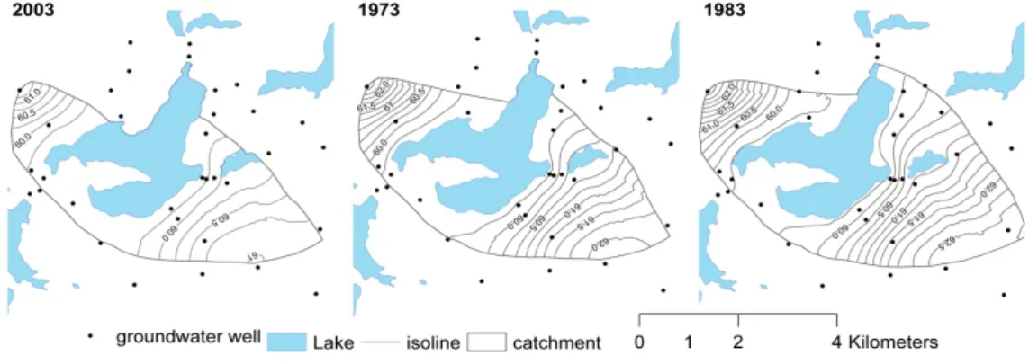
permeability (Ginzel and Kaboth, 1999). However, there is a large variability of the thickness of the unsaturated zone: It is about 0.3 m close to the lake and about 30 m at the outwash plain. Nevertheless, the hydrogeological situation in this area is quite complicated. Holzbecher (2001) could illustrate that the groundwater catchment contracts or extents in dependency on the overall meteorological

conditions (Figure 2.1-3) and measures an average of 11 km². Hence, there are only two areas which constantly deliver groundwater towards the lake: the north-western and south-eastern outwash plains.

Figure 2.1-3: Interpolation of the average annual catchment according to the findings of Holzbecher (2001) for three years with different precipitation condition: dry (2003); average (1973) and wet (1983).

(26)

2.1.3 Oxbow site at the River Spree

At the study site the River Spree (N52°22’06’’ E13°48’25’’) follows the former course of the glacial valley. During the ice age, coarse sandy sediments were accumulated, which were superimposed by fluvial sediments during the Pleistocene (Driescher, 1999). Together, this forms an unconfined aquifer of about 20 m thickness. Since the study site is directly located within the floodplain of the river, the unsaturated zone is very shallow and reaches from 0 of 1.5 m (Lewandowski et al. 2009).

The site can be described as artificial island, which was formed around 1960, when the river was straightened and the meander was cut off. This was done according to melioration measures and resulted in an increase of the surface water discharge and a decrease of the overall groundwater level in the whole area. Since the discharge of the river is also regulated via a weir, the natural discharge is more homogeneous within a year as it would be under natural conditions. The floodplain is used as agricultural meadow.

2.2 Identification of subsurface flow paths & flow systems 2.2.1 Water level fluctuations

Water level measurements are the basis for understanding surface water and groundwater systems.

Even if surface water hydrology and hydrogeology are separate scientific fields, these data were and are always available when answering hydrological questions. The main reason is that water levels are easily measureable parameter providing a lot of information, e.g. about the flow conditions or allowing the determination of subsurface catchments (Hölting and Coldeway, 2009).

Following the law of Pascal for hydrostatic pressure p = ρgh, with the density of the water, the

acceleration of the earth and the water level above a given datum h, it can be seen that water level and hydrostatic pressure directly depend on each other. This implies that processes inducing a change in pressure will also cause a water level change (Todd, 1980). In groundwater the most common process inducing a water level change is groundwater recharge; however there are a lot of other possibilities such as changing atmospheric pressure, tides, earthquakes, irrigation and streamflow (Todd, 1980) with the latter being important for the groundwater–surface water interaction. Some studies show that there is a strong correlation between surface water levels and the water levels in the adjacent

groundwater (e.g. Van Geer, 1987, Seibert et al. 2003; Lewandowski et al., 2009). Lewandowski et al.

(2009) illustrate that this strong correlation is not the result of water transport towards or from the aquifer. Rather the surface water table fluctuations induce pressure waves which are traveling through the aquifer. However, the spread of the pressure wave depends on the period and the amplitude of the

(27)

water level fluctuation as well as on the transmissivity and the storage coefficient of the aquifer (Ferris, 1951). With increasing distance to the surface water the pressure wave dampens.

Hence, analyzing of surface water and groundwater levels in an area where both are closely connected should allow conclusions on the sediment properties an aquifer. This was done by a principle

component analysis for a lowland river floodplain equipped with 15 groundwater observation wells including level loggers and 2 river stages recorders (Lehr et al., 2015, study I).

2.2.2 Nutrients and hydromorphological characteristics

The use of tracers in hydro(geo-)logy to determine flow direction and flow velocity is an accepted and often used scientific method (Davis et al., 1980). There is a wide range of possibilities to do so. Either by adding artificial tracers (e.g. chloride, dye or fluorescein) or using natural tracers (e.g. stable isotopes, nitrate). The main advantages for natural tracers are that they are measurable over a larger range of scales and deliver insights into the spatial and temporal variability of the hydrological system, but beside this they do not disturb the natural conditions of the groundwater flow (Moser, 2004).

However, the application of these kind of tracers requires natural differences in concentrations, e.g. of surface water, soil water, groundwater (Käss, 2004). Therefore, the difference has to be investigated first, before these tracers can be used. Natural tracers are distinguished between: reactive and non- reactive. The first are useful to determine the flow path and the last are more applicable for estimating residence times (Lischeid, 2008).

Nutrient concentrations in the groundwater (e.g. dissolved phosphate, ammonium, and nitrate) depend on: (1) the source (e.g. the amount of degradable organic material, fertilizer), (2) the binding capacity of the sediment (3) the redox conditions, (4) the demand of the vegetation, (5) the temperature and (6) the flow velocity or reaction time, respectively. The concentrations of nutrients in the groundwater can vary a lot and do not fulfill the requirements of a perfect tracer (compare Davis et al., 1980; Käss, 2004). Nevertheless, the spatial distribution of nutrients allow insights into turnover and transport processes, assuming that the temporal variations in shallow aquifers are small in comparison to the spatial variations (compare Bjerg and Christensen, 1992, Lewandowski and Nützmann, 2010, Schot and Pieber, 2012).Accordingly, the flow direction can be estimated.

In study II (Pöschke et al., 2015 b) the distribution of the phosphate and nitrogen concentrations in a shallow floodplain aquifer were related to small scale topography and sediment structure. This was done by multi-level sampling (Graham, 2009) in a vertical spatial resolution of 10^-1 m over a depth range of 2.4 m. The samplers were installed at 6 locations within the floodplain with an average distance of 50 m in between. Additionally, temporary piezometers with a horizontal distance of 3 m

(28)

were installed in the upper meter of the groundwater along a transect. The results were related to a digital elevation model with a spatial resolution of one meter and ground penetrating radar images.

2.2.3 Groundwater modeling

An adequate tool for determining the pattern of groundwater flow from a catchment towards surface water is numerical groundwater modeling. It delivers basic insights on the general distributions of e.g.

flow paths and flow timescales. Moreover, it is helpful for the identification of hydrogeological characteristic areas within the catchment as well as the estimation of the reaction of the hydrological system on different impacts, like climate change or anthropogenic water extraction.

Besides the improved computational opportunities for numerical simulations in the past years, the data basis which can be used for modeling has also increased. Now, long term observations of groundwater and surface water levels allow better identification of system drivers and therefore improve the calibration process (Hill and Tiedeman, 2007). Additionally, the advanced data basis can be used to identify the drivers for changes in subsurface and surface flow processes.

In study III a simple 2D groundwater modeling approach was used to determine the impact of the groundwater leakage into deeper aquifers on groundwater discharge towards Lake Stechlin in NE Germany. At first, a conceptual model was developed to determine the factors driving the groundwater flow towards the lake. Therefore, time series of monthly water levels for lake and groundwater were available from 1957 – 2012. Furthermore, information of topography and geology and meteorological data (precipitation, groundwater recharge) was used. The conceptual model assumes that there is a subsurface flow towards deeper aquifers, due to abrupt changes in the hydraulic gradient in the catchment and measured high hydraulic gradient towards the depth. The implemented numerical model considered different hydraulic conductivities and different leakage areas and leakage amounts into deeper aquifers. At the end the model results were compared to measured groundwater

exfiltration. Furthermore, the realistic model results were analysed for groundwater flow path and changes in the catchment extension.

2.3 Impact of groundwater on surface water 2.3.1 Temperature as tracer

A measured temperature of a gas, fluid or solid matter is a result of the (1) initial temperature, (2) the physical properties of the compartment and (3) the amount of external energy/heat input. There are two important external heat sources for natural water bodies: the natural heat of the earth and the solar

(29)

radiation of the sun. The first is characterized by an almost linear increase of temperature with increasing depth in the subsurface (1°C/ 20 – 40m) (Anderson, 2005). The importance of the geothermal heat source for water bodies depends on the geologic area (geologic active regions vs.

inactive region), the depth of the water body and the thermal properties (e.g. Magri et al. 2015). In contrast, the intensity and temporal variability of the solar radiation depends on the longitude, the continentality and the elevation (Malberg, 1997). In the case of aquatic systems, the physical properties affecting the heat distribution are the heat capacity and conductivity of the water and the surrounding sediment, the velocity and the volume of the water.

Hence, a measured temperature is always a mixed signal of the physical properties and the variability of the heat input source. Still, it is hard to identify the driving parameters which result in the measured value. Therefore, temperature measurements can be addressed as integrative. This provides a usage for different spatial and temporal scales and therefore, it is a useful tool to identify flow pattern in

groundwater (e.g. Stonestrom and Constantz, 2003; Miyakoshi et al. 2003). In the past decades, heat was also used as a tracer to detect groundwater – surface water interactions based on the assumption that groundwater temperatures are more or less constant throughout the year and the surface water underlies an annual temperature cycle (e.g. Schmidt et al. 2006, Anderson, 2005).

Another important characteristic of temperatures is the continuous distribution in time and space. It is always questionable if a point measurement is an adequate representation, especially for flowing systems. Hence, an extensive detection of thermal structures would allow conclusions, if a point measurement were representative for the whole aquatic system at a given scale. One possibility is aerial thermal infrared imagery (TIR) (Beck, 2006). This technique is able to detect thermal patterns at a high resolved spatial scale by temporal snapshots. However, as mentioned before, temperatures are mixed signals and have to be interpreted carefully.

In the present study temperature was used to detect surface temperature pattern within lakes and relate this to a specific process. The first study hypothesized that groundwater discharge areas are detectable by TIR when the groundwater is less dense than the surface water and is floating on the surface and there are windless conditions (Lewandowski et al. 2013; study IV). The second study investigates the effect of the wind on the skin surface temperature distribution. Therefore, two lakes were investigated by TIR, lake surface temperature and temperature depth measurements (Pöschke et al., 2015 a; study V).

(30)

3. Studies

3.1 Survey of studies and authors contribution

Lehr, C., Pöschke, F., Lewandowski, J., Lischeid, G. 2015. A novel method to evaluate the effect of a stream restoration on the spatial pattern of hydraulic connection of stream and groundwater. Journal of Hydrology. 527. 394 – 401.

The first study (I) addresses a larger spatial scale of the same floodplain (100 m). Measured water level of groundwater and surface waters were analyzed by a principle component analysis (PCA) to describe the spatial variability of the hydraulic connectivity between groundwater and surface water (hypothesis 1).

Contribution: I interpreted the results (30%) and wrote the paper (30%).

Pöschke, F., Lewandowski, J., Nützmann, G. 2015. Impact of alluvial structures on small-scale nutrient heterogeneities in near-surface groundwater. Ecohydrology. 8. 682-694

The study (II) is dealing with near surface groundwater in a floodplain aquifer. The small - scale distribution (10 cm to 1 m) of redox sensitive parameters and sediments was used to characterize flow and redox process in a restricted area of a local flow system (hypothesis 1)

Contribution: I conceptualized and designed the study (60%), performed the field work and analytics (70%), interpreted the results (70%) and wrote the paper (80%).

Pöschke, F., Nützmann, G., Engesgaard, P., Lewandowski, J. The hole in the aquifer - effects of groundwater leakage on the local groundwater flow system of a lake (Draft)

The manuscript (study III) present the results of a numerical groundwater modeling approach to estimate the effects of groundwater leaking on the groundwater discharge towards a lake. The results indicate, that leaking might influence the local flow system by reducing the amount of groundwater entering the lake and increases the traveling time of the groundwater. (hypothesis 2).

Contribution: I conceptualized and designed the study (50%), performed the field work and the modeling (80%), interpreted the results (70%) and wrote the paper (90%).

(31)

Lewandowksi, J., Meinikmann, K., Ruhtz, T., Pöschke, F., Kirillin, G. 2013. Localization of lacustrine groundwater discharge (LGD) by airborne measurement of thermal infrared radiation. Remote Sensing of Environment. 138. 119 – 125. DOI: 10.1016/j.rse.2013.07.005

The study (IV) presents a study conducted at a lake with the aim to identify the groundwater

exfiltration areas on the lake surface by thermal infrared imaging at the beginning of lake stratification period (hypothesis 3).

Contribution: I performed the field work (50 %), interpreted the results (20 %) and wrote the paper (10

%).

Pöschke, F., Lewandowski, J., Engelhardt, C., Preuß, K., Oczipka, M., Ruhtz, T., Kirillin, G. 2015.

Upwelling of deep water during thermal stratification onset - A major mechanism of vertical transport in small temperate lakes in spring? Water Resources Research. 51. 9612 – 9627.

The study (V) presents also the usage of thermal infrared imaging. In contrast to Paper III it end up with the result, that wind driven processes predominate the lake surface temperature pattern within two lakes (hypothesis 3).

Contribution: I conceptualized and designed the study (50%), performed the field work (80%), interpreted the results (70%) and wrote most of the paper (65%).

(32)

3.2 A novel method to evaluate the effect of a stream restoration on the spatial pattern of hydraulic connection of stream and groundwater

Christian Lehr^1,2, Franziska Pöschke^3,4, Jörg Lewandowski^3,4, Gunnar Lischeid^1,2

1 Leibniz Centre for Agricultural and Landscape Research (ZALF) Institute of Landscape Hydrology

2 University of Potsdam, Institute of Earth and Environmental Science

3 Institute of Freshwater Ecology and Inland Fisheries, Ecohydrology Department

4 Humbodt University Berlin, Geography Department,

Published in: Journal of Hydrology

Lehr, C., Pöschke, F., Lewandowski, J., Lischeid, G. 2015. A novel method to evaluate the effect of a stream restoration on the spatial pattern of hydraulic connection of stream and groundwater. Journal of Hydrology. 527. 394 – 401.

http://dx.doi.org/10.1016/j.jhydrol.2015.04.075

This is an open access article under the CC BY license (http://creativecommons.org/licenses/by/4.0/)

(33)

Abstract

Stream restoration aims at an enhancement of ecological habitats, an increase of water retention within a landscape and sometimes even at an improvement of biogeochemical functions of lotic ecosystems.

For the latter, good exchange between groundwater and stream water is often considered to be of major importance. In this study hydraulic connectivity between river and aquifer was investigated for a four years period, covering the restoration of an old oxbow after the second year. The oxbow became reconnected to the stream and the clogging layer in the oxbow was excavated. We expected increasing hydraulic connectivity between oxbow and aquifer after restoration of the stream, and decreasing hydraulic connectivity for the former shortcut due to increased clogging. To test that hypothesis, the spatial and temporal characteristics of the coupled groundwater-stream water system before and after the restoration were analyzed by principal component analyses of time series of groundwater heads and stream water levels. The first component depicted between 53% and 70% of the total variance in the dataset for the different years. It captured the propagation of the pressure signal induced by stream water level fluctuations throughout the adjacent aquifer. Thus it could be used as a measure of

hydraulic connectivity between stream and aquifer. During the first year, the impact of stream water level fluctuations decreased with distance from the regulated river (shortcut), whereas the hydraulic connection of the oxbow to the adjacent aquifer was very low. After restoration of the stream we observed a slight but not significant increase of hydraulic connectivity in the oxbow in the second year after restoration, but no change for the former shortcut. There is some evidence that the pattern of hydraulic connectivity at the study site is by far more determined by the natural heterogeneity of hydraulic conductivities of the floodplain sediments and the initial construction of the shortcut rather than by the clogging layer in the oxbow.

(34)

3.2.1 Introduction

In the past decades there has been an increasing effort on research and practice according to the restoration of rivers and their floodplains. The main reasons for that are the valuation of river

ecosystems as place for species conservation and habitat diversity, recreational and aesthetic purposes, flood protection, enhancing the potential of contaminant deposition and nutrient degradation

(Bernhardt et al., 2007; Kondolf et al., 2007; Hester and Gooseff, 2010; Pander and Geist, 2013;

Schirmer et al., 2013). This is also reflected in a growing body of legislative directives (Pander and Geist, 2013; Schirmer et al., 2013), e.g. the EU Water Framework Directive demands a good chemical and ecological status of groundwater and surface water (European Commission, 2000). The chemical and ecological status of surface waters is impacted by the adjacent connected aquifer and vice versa.

Hence both waters have to be considered when assessing water qualities of either of them.

Nevertheless, in river restoration practice the measures most often focus solely on surface waters, whereas the connection of the river and the groundwater below the river bed and the adjacent floodplain is often neglected (Boulton, 2007; Boulton et al., 2010; Hester and Gooseff, 2010).

Previous studies identified the transition zone between stream water and groundwater, the hyporheic zone, as highly relevant for mass exchange, residence time of water and substances in the stream or in the sediment, the chemical and metabolic turnover and in general as crucial for water quality (Brunke and Gonser, 1997; Sophocleous, 2002; Boulton, 2007). The spatial extent of the hyporheic zone is mainly determined by two drivers, the hydraulic gradient between the river and the groundwater and the sediment structure (Kasahara et al., 2009), especially the permeability of the stream bed and aquifer sediments (Woessner, 2000; Kalbus et al., 2009). Therefore, clogging of the stream bed, i.e. the sealing of the stream bed with sediments of very low hydraulic conductivity, has been identified as major problem for exchange of surface water and groundwater and the related ecological functions of the hyporheic zone (Sophocleous et al., 1995; Brunke and Gonser, 1997; Sophocleous, 2002).

Fluxes are spatially and temporally heterogeneous due to the spatial heterogeneity of hydraulic conductivity of the sedimentsand spatial and temporal variability of hydraulic gradients (Woessner, 2000; Malard et al., 2002; Krause et al., 2011; Binley et al., 2013). Different methods are available to estimate fluxes across the interface in a river-groundwater system (Kalbus et al., 2006). Selective approaches, such as vertical temperature profiles (e.g. Schmidt et al., 2006; Anibas et al., 2009), heat pulse sensors (e.g. Lewandowski et al., 2011), hydraulic gradients (e.g. Krause et al., 2012) or seepage meters (e.g. Rosenberry and LaBaugh, 2008) are able to monitor the flux over time for a specific point, but it is not possible to draw conclusions for a whole river section.

A method to capture larger areas is distributed temperature sensing (DTS) (e.g. Selker et al., 2006a,b;

Krause and Blume, 2013), which is able to detect spots with intense groundwater ex- and infiltration.

Another option is to use natural or artificial tracers to determine the degree of interactions (e.g. Négrel

Approaches to identify groundwater discharge towards and within lowland surface water bodies on different scales