Analysis of Flow and Transport in Refractive Index Matched Porous Media

(1)

Dissertation submitted to the

Combined Faculties for the Natural Sciences and for Mathematics of the Ruperto-Carola University of Heidelberg, Germany

for the degree of Doctor of Natural Sciences

presented by

Diplom-Physicist Michael St¨ohr born in Stuttgart

Oral examination: 22nd July 2003

(2)

(3)

Analysis of Flow and Transport in Refractive Index Matched Porous Media

Referees: Prof. Dr. Kurt Roth Prof. Dr. Bernd J¨ahne

(4)

(5)

1

Zusammenfassung

In der vorliegenden Arbeit wurde eine neuartige Methode zur Messung von Strömung und Transport in porösen Medien entwickelt. Durch die Verwendung von speziell geeigneten Fest- stoffen, Flüssigkeiten und fluoreszierenden Farbstoffen sowie die Anwendung eines hochge- nauen Verfahrens zur Anpassung der Brechungsindizes konnte die Dynamik der Farbstoff- verteilung in einem dreidimensionalen porösen Medium mittels planarer laser-induzierter Fluoreszenz mit einer sehr hohen zeitlichen und räumlichen Auflösung bestimmt werden.

Für die Auswertung der Daten wurden speziell angepasste Algorithmen zur Bildvorverar- beitung entwickelt sowie ein Verfahren zur lokalen Parameterschätzung auf die vorliegende Anwendung übertragen und entscheidend erweitert. Die durchgeführten Messungen stellen die erste gleichzeitige Bestimmung des longitudinalen sowie der beiden transversalen hydrody- namischen Dispersionskoeffizienten dar. Während für die longitudinale Dispersion ein bereits bekanntes Potenzgesetz bestätigt wurde, konnte für die transversale Dispersion erstmals ein deutlich unterschiedliches Verhalten in vertikaler und horizontaler Richtung nachgewiesen werden. Weiterhin konnte mit dem entwickelten Verfahren erstmals der direkte Nachweis für die Existenz nicht konvektiver Zonen, die einen wichtigen Teil zur Dispersion beitragen und eine mögliche Erklärung für das Verhalten gemäß eines Potenzgesetzes bieten, erbracht werden. Schließlich wurde mit dem Verfahren erstmals die Strömung zweier nicht mischbarer Flüssigkeiten in einem dreidimensionalen porösen Medium hochaufgelöst visualisiert.

Abstract

In the present work a novel method for the measurement of flow and transport in porous media has been developped. Through the employment of particularly applicative solids, liquids and fluorescent dyes and the application of a method for the highly precise matching of refractive indices, the dynamics of the dye distribution inside a threedimensional porous medium could be determined with a high temporal and spatial resolution using planar laser-induced fluorescence. For the data analysis specifically adapted algorithms for image preprocessing have been developed and a method for local parameter estimation has been adapted and significantly enhanced for the present application. The performed measurements represent the first simultaneous estimation of the longitudinal and both transversal hydrodynamic dispersion coefficients. Whereas for the longitudinal dispersion a previously known power-law could be confirmed, the significantly different behavior of the transversal dispersion in vertical and horizontal direction has been observed for the first time. Furthermore the measurements provide the first direct evidence for the existence of stagnant zones in the liquid phase, which have an important effect on the dispersion and are a potential explanation for the power-law behavior. Finally the described technique was used for the first highly resolved visualization of the flow of two immiscible liquids in a threedimensional porous medium.

(6)

(7)

Chapter 1 Introduction

The study of ﬂow and transport in porous media is an active ﬁeld of research, which has applications in many disciplines such as

• forecast of transport and fate of water, dissolved contaminants and non-aqueous phase liquids in hydrology

• heterogeneous catalysis in chemical engineering

• oil recovery in petroleum engineering

• ﬂow of blood and other body tissues in biochemistry and medicine.

The scientific challenge in all these fields is the development of appropriate models for flow and transport, which can then be used e.g. to predict the spreading of a contaminant in an aquifer or to optimize the reaction rate in a packed bed. There is a general agreement among scientists and engineers across the disciplines that further progress in the modeling of these phenomena can only be achieved through the development of enhanced and new experimental techniques.

Earlier studies mostly treated the porous medium as an effectively homogeneous system and neglected the complexity and variability of the local flow processes within the porous medium. It is not surprising that the predictions of models which are based on such simple approaches often proved false. The restriction to the employment of these simple models, mainly caused by the lack of experimental methods for the visualization and quantification of local structure and dynamic processes, could lately be relaxed by the emergence of capable new measurement instrumentation. As a consequence, the models become more sophisticated making use of the contemporaneously growing power of the computers used for their solution.

The spread and fate of water, dissolved contaminants and non-aqueous phase liquids in hydrology is governed by dynamic processes acting on many diﬀerent scales. From this follows the demand for a variety of experimental methods in order to measure each of these processes on its characteristic scale. Currently progress is made by the development of X- ray tomography, nuclear magnetic resonance (NMR) imaging and refractive index matching techniques on the laboratory scale, ground penetrating radar (GPR) on the ﬁeld scale and remote sensing with aircrafts and satellites on the global scale.

The objective of this work is the development and application of a planar laser induced ﬂuorescence (PLIF) technique for the spatially and temporally highly resolved measurement

(12)

CHAPTER 1. INTRODUCTION

of flow and transport in refractive index matched porous media. Being part of the gradu- ate program ’Modelling and Scientific Computing in Mathematics and Natural Sciences’ at the Interdisciplinary Center for Scientific Computing (Interdisziplinäres Zentrum für Wis- senschaftliches Rechnen, IWR) of the University of Heidelberg, it benefited from the parallel affiliations to both the soil physics group at the Institute of Environmental Physics and the digital image processing group at the IWR. Followingly it was performed in view of the impli- cations mainly for hydrological models and with the claim to develop sophisticated methods for the processing of the measured data and parameter estimation.

(13)

Chapter 2 Theory of Hydrodynamic dispersion

2.1 Introduction

The basic approach to the description of ﬂow and transport in porous media is the introduction of appropriate scales and the derivation of adequate physical models for each scale. This concept is illustrated in ﬁgure 2.1: On each scale the respective physical model has a set of intrinsic parameters, which contain structural and material properties. The determination of the correct physical models (like e.g. kinetic theory or Navier-Stokes-equation) for each scale is accomplished through the intuition of (a) scientist(s) from the analysis of experimental observations. Furthermore it is sometimes possible to relate the parameters at a given scale to the model and the parameters at the next smaller scale, a procedure usually referred to as upscaling. Such a relation can be an analytical equation obtained from intuition or an empirical law obtained from the analysis of experimental data.

In this sense the theory of hydrodynamic dispersion will be presented in the following sections as a sequence of transitions from the scale of a single molecule to the scale of an aquifer as illustrated in figure 2.1. The first transition presented in section 2.2 goes from kinetic theory to the continous formulation of molecular diffusion, which was accomplished by Albert Einstein in 1905. The phenomenon of hydrodynamic dispersion is then introduced in section 2.3 as a transition from the transport model for a pure stagnant liquid to a model for the transport in a liquid flowing through a porous medium. This transition is characterized by a strong enhancement of the transport efficiency (typically orders of magnitude), which is caused by a combination of several microscopic physical processes, which are addressed in detail in section

2.2 From kinetic theory to molecular diﬀusion

The phenomenon of molecular diffusion sketched in figure 2.2a-c is well-known from everyday life: a small pulse of dye (e.g ink) injected into a box of water changes its shape with time towards a broader distribution without any active external stimulation. The first successful explanation of this phenomenon was provided by the kinetic theory developed in the middle of the 19th century by Rudolf Clausius, James Clerk Maxwell, Ludwig Boltzmann and others.

At this time a similar phenomenon was known under the name brownian motion after the Scottish botanist Robert Brown (1773-1858). In 1827 he observed the zig-zag motion of pollen grains suspended in water under a microscope (Brown, 1828).

(14)

CHAPTER 2. THEORY OF HYDRODYNAMIC DISPERSION

Scale

Molecular Scale

Continuum scale of hydrodynamics and molecular diffusion

Continuum scale of hydrodynamic dispersion in a homogeneous porous medium

Physical model

Kinetic Theory (Newton's laws + Probabilistic theory)

Navier-Stokes- equation (Flow) Fick's laws (Transport)

Darcy's law (Flow) Convection-dispersion- equation(Transport)

Parameters

Molecule Radius R

Viscosity η

Hydraulic conductivity K Dispersion tensor D Diffusion

coefficient D

Molecule mass mStokes-Einstein-relation

{ {

D(D , d, η, ...) m

m

Porosity φ

Figure 2.1: Concept of the description of physical processes on diﬀerent scales. On each scale, the processes are described by an adequate physical model and a set of intrinsic parameters.

The major scientiﬁc challenge, besides the determination of the correct physical models, is the derivation of the relations between the models and parameters for diﬀerent scales. The purpose of this illustration is not to provide any complete description (which would have to include temperature dependence, compressibility etc.), but rather to present the conceptual idea of scale transitions.

(15)

2.2. FROM KINETIC THEORY TO MOLECULAR DIFFUSION

t

₁

t

₂

t

₃

Figure 2.2: Diffusion of a dyed solute pulse in a transparent solvent: the diffusion coefficient Dmfor the description of the physical process on the continuum scale (a-c) can be related to the properties of the molecular scale (d) through the Stokes-Einstein-equation 2.8.

Kinetic theory, which is based on the main assumptions

• All matter is composed of small particles.

• The particles are in constant motion according to Newton’s law.

• The collisions between the particles are perfectly elastic.

correctly explains these phenomena by the equipartition of thermal energy resulting in a permanent process of movement and collisions of the particles.

During the same time, the young Adolf Fick (1831-1879), a physiologist at the University of Zürich wrote a work entitled ” Über Diffusion” (On Diffusion, Fick (1855)). Starting from his interest in diffusion through organic membranes, he addressed himself to the study of diffusion of a solute in its solvent as the elementary physical process. Therefore he performed a series of quantitative measurements of the diffusion of sodium chloride aqueous solutions contained in cylindrical jars together with pure water.

In contrast to kinetic theory, he came up with a phenomenological description based on the empirically obtained assumption that the currentj is proportional to the concentration gradient,

j=−D_m∇c, (2.1)

an equation now known as Fick’s first law. Here c denotes the concentration and D_m is the coefficient of molecular diffusion. The additional assumption that the particles are neither created nor destroyed leads to the continuity equation

∂c

∂t =−∇ · j. (2.2)

The combination of Fick’s ﬁrst law and continuity equation leads to Fick’s second law

∂c

∂t =Dm∆c. (2.3)

Although Fick was aware of the results of kinetic theory, it took about one half of a century to combine the probabilistic, microscopic description of kinetic theory with the macroscopic

(16)

phenomenological description introduced by Fick. In 1905 it was Albert Einstein (1879-1955) who derived the diﬀusion equation 2.3 from the postulates of kinetic theory by realizing that the particle concentrationc(x, t) is proportional to the probabilityp(x, t) of ﬁnding a particle at (x, t) (Einstein, 1905). The temporal evolution of p(x, t) for a particle initially released at the origin of a d-dimensional space can then be obtained as the normalized solution of equation 2.3,

p(x, t) = 1

(4πD_mt)^d/2e⁻ ^r

2

4Dmt, r²=x², (2.4) and thus the mean squared displacement of the particle grows linearly with time:

r²(t)=

r²p(x, t)d³r= 2dD_mt. (2.5) Furthermore Einstein has shown that the diﬀusion coeﬃcientD_mfor a solute is the ratio of the mean thermal energy of the medium kT and the friction f between the solute and the solvent,

Dm= kT

f . (2.6)

Stokes has shown that the friction of a spherically shaped particle of radius R in a solvent with viscosity η is given by

f = 6πηR. (2.7)

From this relation Einstein calculated the diﬀusion coeﬃcient D_m as Dm= kT

6πηR, (2.8)

which is today calledStokes-Einstein-relation. Einstein used this relation to estimate the size of molecules (Einstein, 1906), while at this time the atomistic structure of matter was still a controversial issue (Renn, 1997). In the present work theStokes-Einstein-relation2.8 is used to estimate the diffusion coefficients and Schmidt numbers for different silicone oil mixtures as described in section 8.2.

In the context of the concept of scale transitions introduced in the previous section and illustrated in figure 2.1, the Stokes-Einstein-relation provides an essential link between the description on the molecular scale given by kinetic theory (figure 2.2d), and the description on the continuum scale given by Fick’s laws (figure 2.2a-c).

2.3 From molecular diﬀusion to hydrodynamic dispersion in a homogeneous porous medium

In this section a formalism will be presented for the description of the transport of a solute dissolved in a liquid flowing through a homogeneous porous medium. This is accomplished through an adequate upscaling of the continous description for the diffusive transport in a pure stagnant liquid given by Fick’s laws to an effective description of transport on a properly chosen macroscale. The transport on this macroscale, which is typically caused by a combination of several physical processes, like e.g. diffusion, convection, adsorption or holdup in stagnant zones, is usually referred to ashydrodynamic dispersion.

(17)

2.3. FROM MOLECULAR DIFFUSION TO HYDRODYNAMIC DISPERSION In principle, the temporal evolution of the solute concentration distribution c(x, t) in a liquid ﬂowing through a porous medium can be obtained from the velocity ﬁeld v(x) given by the solution of the Navier-Stokes-equation (see e.g. Tritton (1988))

ρ(∂v

∂t +v·∇v) =−∇p+η∆v+f_external. (2.9) For numerical studies of ﬂow in porous media, which is mostly in the range of low Reynolds numbers Re<1, this equation is often approximated by the linear, and therefore computa- tionally more convenientStokes-equation

ρ∂v

∂t =−∇p+η∆v+fexternal. (2.10)

Subsequentlyc(x, t) is calculated as the solution of the so-calledconvection-diﬀusion-equation

∂c

∂t+∇ · (vc)−D_m∆c= 0, (2.11)

which is a generalization of Fick’s second law 2.3 with the additional term ∇ · (vc) for the convective transport in a ﬂowing liquid.

There are at least two reasons why this approach is not feasible:

• The complex geometry of a porous medium, like e.g. a column ﬁlled with sand or an aquifer, can generally not be obtained. Therefore no solution of the Stokes-equation 2.10 can be calculated due to the lack of boundary conditions.

• Even if the boundary conditions were available, no analytical solution of equations 2.10 and 2.11 would be possible, and the computational requirements for a numerical solution would exceed every imaginable dimension.

However, in many cases the exact solution of equations 2.10 and 2.11 is not necessary, and the complex geometry of the porous medium can be represented by a set of few so-called effective parameters. In the following this approach will at first be exemplarily introduced for the flow in a capillary tube and then extended to the hydrodynamic dispersion in a homogeneous porous medium.

2.3.1 Taylor dispersion

The description of flow and transport in a capillary tube is an illustrative example for the scale transition from molecular diffusion to hydrodynamic dispersion. Due to its simplicity an exact analytical solution for the velocity fieldv(x) is available, and it is further possible to derive exact analytical relations between the microscopic and the effective macroscopic parameters.

The laminar ﬂow ﬁeld in a capillary tube of length L is given by the solution of the Navier-Stokes-equation 2.9 (the so-calledHagen-Poisseuille’s law) as

v(r) = ∆p L

R²

4η(1− r² R²)^v⁰⁼

∆pR2

=4ηL v₀(1− r²

R²), (2.12)

where R denotes the tube radius, r = y²+z² the distance from the central axis of the tube, ∆p the pressure diﬀerence between the tube ends, η the viscosity of the liquid and v₀

(18)

the velocity in the center (r = 0) of the tube. The temporal evolution of the concentration distributionc(x, t) for a dissolved solute with the molecular diffusion coefficient Dm is then described by the convection-diffusion-equation 2.11.

Figure 2.3 shows the evolution of c(x, t) for a solute pulse which was initially uniformly distributed at x = 0 (c(x,0) = c0δ(x)). In this numerical simulation the concentration c is represented by the density of the tracer particles, which are translated by an additive superposition of convective and diﬀusive transport according to

x_t+1=x_t+v(x_t) +ε with ε= 0, ε²= 2D_m. (2.13) From the examination of the images in figure 2.3b-g and the analysis of the governing equations 2.12 and 2.11, the qualitative behavior of solute transport can be separated into two different regimes. The transition between these two regimes is characterized by the time τ a particle needs to diffuse a distance equal to the tube diameter d= 2R:

τ = d²

2D_m = 2R²

D_m. (2.14)

For the simulation shown in figure 2.3 the value of this characteristic time is τ = 40000. For t < τ, the initial transverse positions of the particles have moved less than the tube diameter, and thus the shape of the parabolic flow profile v(r) is still more or less identifiable from the particle distribution. Fort > τ molecular diffusion has led to a complete transverse mixing of the tracer particles and consequently the particle distribution is independent of the transverse position.

Another qualitative change between the behaviors for t < τ and t > τ can be recognized from the temporal evolution of the particle distributions in flow direction, which are represented by the gray lines in figure 2.3b-g: the transition fromt < τ tot > τ is accompanied by a transition of the particle distribution in flow direction towards a gaussian distribution. This important finding is a direct consequence of the so-calledcentral limit theorem(CLT). It essen- tially states that the sum Ω ofnstatistically independent random variablesε_i characterized by their meansµi and variancesσ²_i

µ_i =ε_i and σ²_i =(ε_i−µ_i)² (2.15) is a random variable whose probability distribution converges for n → ∞ to a gaussian distribution with mean µΩ and varianceσ_Ω²:

Ω = n i=1

εi n→∞→ µ_Ω = n i=1

µi, σ_Ω² = n i=1

σ²_i. (2.16)

For a detailed discussion and a proof of this theorem see Grimmett & Stirzaker (2001).

Consequently the 3D microscopic convection-diﬀusion-equation 2.11 converges for t > τ to the 1D macroscopic, so-called convection-dispersion-equation

∂c

∂t +v∂c

∂x−D∆c= 0. (2.17)

The parameters v and D of this macroscopic equation can be directly related to the microscopic flow field v(r) and diffusion coefficientD_m:

v = v0

2, D=Dm+ R²v₀²

48D_m. (2.18)

(19)

2.3. FROM MOLECULAR DIFFUSION TO HYDRODYNAMIC DISPERSION

−0.1 0 0.1 0.2 0.3 0.4 0.5

−1 0 1

y

0 0.02 0.04 0.06 0.08 0.1 0.12

−1 0 1

y

0 0.2 0.4 0.6 0.8 1 1.2

−1 0 1

y

0 2 4 6 8 10 12

−1 0 1

y

0 20 40 60 80 100 120

−1 0 1

y

0 200 400 600 800 1000 1200

−1 0 1

y

0 2000 4000 6000 8000 10000 12000

−1 0 1

x

y

t=1 t=0

t=10

t=100

t=1000

t=10000

t=100000 a

b

c

d

e

f

g

v₀=0.1 D_m=5 ⋅ 10⁻⁵

Figure 2.3: Dispersion of a solute pulse in the flow field of a capillary tube: fort > τ = 40000 the particle distribution in flow direction (indicated by the gray lines) approaches a gaussian distribution according to the central limit theorem. The images represent the 2D projections of the 3D particle distributions.

(20)

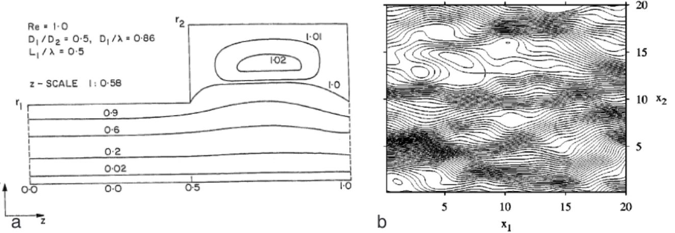
Figure 2.4: Steady flow field in an array of spheres obtained from the solution of the Stokes- equation 2.10 using a finite difference method (reprinted from Rage (1996)).

In recognition of Sir Geoﬀrey Taylor, who found these relations in 1953 (Taylor, 1953), the dispersion of a solute in a capillary tube is today usually referred to asTaylor-dispersion.

The transport on the macroscale , which is caused by a combination of microscopic convection and diffusion, is quantified by the dispersion coefficient D. According to equation 2.18, the value of D is typically significantly higher than Dm. At first view it is surprising that D decreases with increasing D_m. This is a result of the effect that a high value of D_m increases transverse mixing and therefore reduces the broadening of the particle distribution in flow direction due to convection.

Although the flow in a capillary tube is mostly not an adequate model for the flow in a porous medium, the observed mechanisms and the resulting description by a macroscopic convection-dispersion-equation provide the conceptual basis for the following description of flow and transport in a porous medium.

2.3.2 Hydrodynamic dispersion in a homogeneous porous medium

In contrast to the flow in a capillary tube, the exact flow field in a porous medium is typically not known. Numerical solutions like that shown in figure 2.4 are only feasible for small do- mains and only under the condition that the boundary conditions, i.e. the shape of the solid surfaces, are known. However, even if these conditions are not fulfilled and the detailed velocity profile is not available, thecentral limit theorem, which was applied for the macroscopic description of transport in a capillary tube, is in principle similarly applicable to the flow in a porous medium.

The transition from the microscopic description based on the Navier-Stokes-equation 2.9 and the convection-diﬀusion-equation 2.11 to the macroscopic description of ﬂow and transport in homogeneous porous medium based on the central limit theorem then leads to the 3D

(21)

convection-dispersion-equation

∂c

∂t+∇ · (vc)−∇ · (D ∇c) = 0. (2.19) Here v denotes the macroscopic averaged velocity in the liquid phase and

D=





D_xx D_xy D_xz D_xy D_yy D_yz Dxz Dyz Dzz



 (2.20)

denotes the symmetric so-calleddispersion tensor. For the ﬂow in x-direction (v= (v_x,0,0)^T) in an isotropic porous medium, D is given by

D=





D_L 0 0

0 D_T 0

0 0 DT



, (2.21)

where D_L and D_T are the so-called longitudinal and transversal dispersion coeﬃcients. The value ofv can be obtained from the solution of the Darcy equation

v=−K

η ∇p, (2.22)

whereηdenotes the liquid viscosity andKis thehydraulic conductivityof the porous medium.

For many practical applications of flow and transport in porous media (like e.g. the spread and fate of contaminants in an aquifer) the values of D_L,D_T andK are an essential information. However, unlike the above discussed flow in a capillary tube, no analytical relations are available here due to the complexity of the porous medium. WhereasK is only a function of the porous structure, the dispersion coefficientsD_L andD_T potentially depend on many different parameters of the porous matrix, the solvent and the solute, like e.g. the macroscopic velocity v, the particle diameter d (as a first-order representation the pore geometry), the densityρ and viscosity η of the solvent and the diffusion coefficientD_m:

D_L/T=D_L/T(v, d, ρ, η, Dm, . . .) (2.23) The analysis of the geometrical and dynamical similarity of the functional dependence 2.23 according to the Buckingham-Pi-theorem (Buckingham, 1914) leads to the conclusion that the dimensionless dispersion coeﬃcients _D^D_m^L and _D^D^T_m can be written as a function of two dimensionless variables:

D_L/T Dm

= D_L/T Dm

(vd Dm

, η ρDm

, . . .) = D_L/T Dm

(Pe,Sc, . . .) (2.24) Although in principle other dimensionless variables could be chosen, the above used Peclet numberPe andSchmidt numberSc are the by far most common. Intuitively the Peclet number represents the relative magnitudes of convective and diffusive transport over the typical length d of the porous medium, and the Schmidt number represents the ratio of the coefficents of momentum diffusion and mass diffusion:

Peclet number Pe = vd

D_m = ”convective transport”

”diﬀusive transport” . (2.25)

(22)

a b

Figure 2.5: Dependence of the dimensionless longitudinal dispersion coefficient _D^D_m^L on the Peclet number Pe represented by a compilation of measurements from several authors reprinted from a Dullien (1992) and b Sahimi (1993) including a classification of different Pe ranges.

Schmidt number Sc = η

ρD_m = ”momentum diﬀusion”

”molecular diﬀusion” . (2.26) The transformation of constitutive equations into a dimensionless form is a commonly used method to reduce a physical process to its intrinsic complexity, especially in hydrodynamics.

A more detailed discussion of this concept is given in Tritton (1988).

For several decades it is the objective of both theoretical and experimental scientists to determine the dependencies of the dispersion coefficients on the Peclet number and Schmidt number. For the experimental studies substantial use is made of the dimensionless formulation 2.24: the existence of this formulation provides the opportunity to study the (Pe, Sc)-dependence of the dispersion coefficients through comparatively inexpensive laboratory experiments. The values of the dispersion coefficients can then in principle be transformed to any other scale, like e.g. the field scale in hydrology.

Figure 2.5 shows two compilations of experimentally determined longitudinal dispersion coefficients plotted versus the Peclet number Pe. According to Sahimi (1993) the dependence of _D^D_m^L on Pe can be broken down into five different regimes as indicated in figure 2.5b:

Pe < 0.3

In this regime convection is so slow that dispersion is controlled almost completely by diﬀusion.

Consequently the dispersion is isotropic with the dispersion coeﬃcients given by DL

Dm

= DT

Dm

= 1

F φ, (2.27)

where F is the so-called formation factor and φ the porosity of the porous medium. The value of _{F φ}¹ , which is determined by the pore structure, is typically in the range between 0.15 and 0.7.

(23)

0.3 < Pe < 5

This regime is characterized by the transition from the diffusion-dominated regime to a regime mostly controlled by convection. In this transition zone, where both diffusion and convection contribute significantly to the dispersion, the dispersion coefficients start to increase with increasing Pe. However, no universally valid formula for ^D_D^L_m^/^T(Pe) has yet been obtained for this transitional regime.

5 < Pe < 300

In this range of Peclet numbers, the so-called power-law regime, the measured dispersion coeﬃcients are best described by the empirical relations

DL

D_m =αLPeⁿ^L and (2.28)

D_T

D_m =α_TPeⁿ^T. (2.29)

A comparison of experimentally obtained values for αL, αT, nL and nT is given in section 8.3.2. A theoretical consideration of this behavior is presented in section 2.3.3.

300 < Pe < 10⁵

For a porous medium without any stagnant zones, like e.g. dead-end pores (see section 2.3.3), the transport in this Pe range is completely dominated by convection (usually referred to as mechanical dispersion) and thus the dependence on the Peclet number must be linear:

D_L

D_m =α_LPe and (2.30)

DT

Dm

=αTPe. (2.31)

However, there are strong indications that stagnant zones are much more prevalent in porous media than intuitively expected (see section 8.3.5). This leads to an extension of the power- law relations 2.28 and 2.29 into the present Pe range, which is conﬁrmed by the results of several authors given in section 8.3.2.

Pe > 10⁵

Whereas for the previous Pe regimes a laminar flow field was assumed, in this regime turbu- lence starts to contribute to the dispersion process. Consequently the dispersion coefficients are supposed to depend not only on the Peclet number Pe, but also on the Reynolds number Re =^ρ^vd_η .

The plot of the longitudinal dispersion coefficients versus the Peclet number in figure 2.5a, which is compiled from measurements using a large variety of porous media, solvents and solutes and therefore covering a large range of values for d, ρ,η and D_m, suggests that the dispersion coefficients depend solely on the Peclet number, and the dependence on the Schmidt number can be neglected. In one of the few quantitative studies of the Schmidt number dependence of dispersion coefficients, Delgado & Guedes de Carvalho (2001) have found that ^D_D_m^T shows a dependence on Sc only for Sc<550.

(24)

2.3.3 Theoretical models

The following paragraphs are designed to provide a more detailed analysis of the microscopic physical processes that lead to the empirical laws for the respective Pe ranges which have been discussed above. Koch & Brady (1985) have developped a quantitative theory which states that the dispersion coeﬃcients are resulting from a combination of the following physical phenomena:

• In the absence of convection, the dispersion coefficients are given by the tortuosity τ of the porous medium, which is defined as the ratio of D_L/T at Pe= 0 and the diffusion coefficient in the pure solventD_m.

• Pure convection results in a contribution to D_L/T which scales linearly with Pe. This so-calledmechanical dispersioncomes from the velocity ﬂuctuations in the liquid phase of the porous medium as illustrated in ﬁgure 2.4.

• The diﬀusive boundary-layers near the solid surface lead to the so-calledboundary-layer dispersion which scales as Pe ln Pe.

• Regions in the liquid phase with zero velocity (so-called stagnant zones), where the solute can enter or exit solely through diﬀusion, lead to a contribution which grows quadratically with Pe. This eﬀect is called holdup dispersion.

Finally the dispersion coeﬃcients are given by the linear superposition D_L/T

Dm

=τ +αPe +βPe ln Pe +γPe². (2.32) According to Koch & Brady (1985), boundary-layer dispersion and holdup dispersion can be neglected for the transverse dispersion coeﬃcients, so that β = 0 and γ = 0 for D_T. The individual contributions are speciﬁed in the next paragraphs.

Tortuosity

As discussed above, the tortuosityτ determines the dispersionD₀ =D_L/T(Pe = 0) of a solute in the absence of convection, and consequently itself is determined by the structure of the pore space. Millington & Quirk (1960) (cited by Roth (1996a)) have found diﬀerent empirical models for the dependence of D₀ on the volumetric content of the liquid phase θ and the porosity φ (θ = φ for saturated porous media). According to Jin & Jury (1996) (cited by Roth (1996a)), Millington-Quirk’s ﬁrst model

τ = D0(θ) D_m = θ

φ^2/3 (2.33)

agrees best with experimental data.

Mechanical dispersion

Mechanical dispersion is the result of the velocity ﬂuctuations in the liquid phase. If the velocity proﬁle v(x) in the porous medium is described statistically by its mean v and its velocity autocorrelation function (VACF)

C_vv(t) =(v(0)−v)(v(t)−v)^T, (2.34)

(25)

a b

Figure 2.6: Diﬀerent types of regions in the liquid phase which are accessible solely by diﬀu- sion: adead-end pore and b circulation pattern.

the time-dependent dispersion tensorD can be calculated as D(t) =

_t

0

C_vv(t)dt. (2.35)

Obviously the asymptotic dispersion tensor D(t→ ∞) only exists if the integral in equation 2.35 converges, i.e. if the VACF decays at least with 1/t. Lowe & Frenkel (1996) have found from numerical simulations using a lattice boltzmann method that at high Peclet numbers the dispersion coeﬃcient is diverging. However, the results of the comparative study of Maier et al. (2000) was contrary to this ﬁnding, and the statement was relinquished by Capuani et al. (2003).

Holdup dispersion

The effect of holdup dispersion results from stagnant zones in the liquid phase of the porous medium, which are accessible from the convective part of the flow field only by diffusion. Since its contribution to the dispersion coefficient grows quadratically with Pe, holdup dispersion is an important mechanism for high Peclet numbers. Intuitively it seems that such stagnant zones like e.g. so-called dead-end pores (figure 2.6a) should hardly occur in unconsolidated bead packings, which are commonly used for laboratory experiments. There are however several studies (including this work) which indicate that holdup dispersion plays an important role in solute transport. A detailed discussion of this issue is given in section 8.3.5.

A possible explanation for the unexpectedly strong influence of holdup dispersion might be the existence of closed loops in the convective flow field. Figure 2.6b shows a potential constellation for the formation of such closed loops. Furthermore Azzam & Dullien (1977) have shown that closed loops can emerge also in rectangular pockets as shown in figure 2.7a.

Dentz et al. (2003) showed analytically that in any incompressible Gaussian random field there is finite probability for closed streamlines (see figure 2.7b).

Boundary-layer dispersion

The following description of boundary-layer dispersion is adopted from Koch & Brady (1985):

”Saﬀman (1959) modelled the microstructure of a porous medium as a network of capillary

(26)

a b

Figure 2.7: aFormation of closed streamlines in a rectangular pocket adjacent to a capillary tube (reprinted from Azzam & Dullien (1977)). bClosed streamlines obtained by Dentzet al.

(2003) from a linearized solution of the Darcy equation for a 2D Gaussian-distributed velocity ﬁeld.

tubes of random orientation. At high Peclet number and at very long time, Saffman found that the dispersion never becomes truly mechanical, the effective diffusivity growing as Pe ln Pe.

The logarithmic dependence results from the zero velocity of the ﬂuid at the capillary walls.

The time required for a tracer particle to leave a capillary would become infinite as its distance from the walls goes to zero, if molecular diffusion did not allow the tracer to escape the region of low velocity near the wall. This phenomenon is similar to the ’holdup’ dispersion mentioned above, although in this case there is no finite region of zero velocity.”

Boundary wall eﬀects

The presence of the boundary walls of the laboratory columns used for the measurements of dispersion coefficients leads to inhomogeneities of the pore structure near the walls. Maier et al. (2002) found that these inhomogeneities lead to a significant increase of the effective longitudinal dispersion coefficient compared to the bulk. Consequently this effect is a possible explanation for deviations between the measured dispersion coefficients from different experiments. Furthermore the adequate consideration of this effect is mandatory for the correct upscaling of the laboratory measurements to the field scale.

2.4 Heterogeneous porous media

The homogeneity of the porous medium was a stringent requirement for the description of flow and transport given in the previous section. This requirement is fulfilled if there exists a finite representative elementary volume (REV) for which the average of the relevant microscopic quantities, like e.g. the velocityv = _V¹ v(x)dV or the porosity φ = _V¹ φ(x)dV, becomes independent of the position x in the porous medium. While the assumption of homogeneity is approximately justified for most unconsolidated bead packings used for laboratory experiments (for a fundamental discussion of this issue see Torquato et al. (2000)), natural porous media like soil are typically heterogeneous on every scale.

(27)

2.4. HETEROGENEOUS POROUS MEDIA

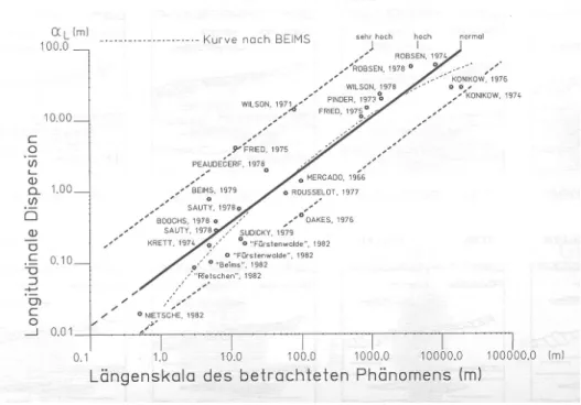
Figure 2.8: Scaling of the longitudinal dispersivity α_L with the length-scale of the solute plume according to Beims (1983) (reprinted from Paus (1997)).

For such porous media no asymptotic dispersion tensor can be found since the integral in equation 2.35 fort→ ∞does not converge. Since with increasing plume size more large-scale heterogenities contribute to the dispersion, the dispersion coeﬃcients increase with the plume size, or equivalently with time. Consequently the dispersion is described by a convection- dispersion-equation with a time-dependent dispersion tensor D(t). The scaling behavior of D(t) strongly depends on the type of the heterogeneites. Figure 2.8 shows the scaling of the longitudinal dispersivity αL with the length-scale of the solute plume for the dispersion in aquifers according to Beims (1983). While at the scale of 1 meter only stones or small clay lenses contribute to dispersion, the large-scale geological morphology leads to a strong increase of αL. Even though the double-logarithmic plot suggests a power-law relation, the conﬁdence bounds are very large.

(28)

(29)

Chapter 3 Method of measurement

3.1 Introduction

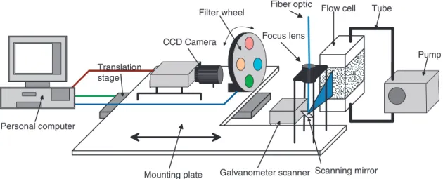
This chapter describes the setup of an experimental apparatus for the non-invasive optical measurement of 3D pore-scale flow and transport in porous media. The method uses a planar laser-induced fluorescence (PLIF) technique in combination with a system of transparent solids and liquids with highly precise matched refractive indices. In PLIF a fluorescent substance is excited by a planar laser sheet with its wavelength tuned to the absorption band of the substance. The light is absorbed by the substance and re-emitted at characteristic wavelengths. A 2D image of the concentration distribution can be obtained by a CCD camera mounted with its optical axis perpendicular to the laser sheet. Due to the fact that the absorption and emission bands of the fluorescent dye have no or only little overlap, the dye distribution between the laser sheet and the camera does not affect the measurement. There- fore a consecutive displacement of the laser plane in the out-of-plane direction results in a set of 2D images representing the 3D concentration distribution. This technique gives access to 3D information without any challenging tomographic reconstruction. The main features of the method, i.e. its high spatial and temporal resolution and the simultaneous visualisation of two immiscible liquids, are attained by the employment of capable illumination and imaging devices and the composition of a proper combination of solids, liquids and fluorescent dyes.

At first the next section gives a short overview of previously employed refractive index matching methods. Then section 3.3 describes the general arrangement of the setup and the technical specifications of the single components used in this work. The physical and chemical properties of the utilised solids, liquids and dyes are specified in section 3.4, 3.5 and 3.6 respectively. Finally a summary and conclusions are given in section 3.7

3.2 Refractive index matching methods

The difficulties of many experimental methods to probe flow and transport on the pore scale of a porous medium, stemming from the opaqueness of the medium, can be overcome by the application of a transparent porous matrix and liquids with their refractive index matched to that of the matrix. Refractive index matching methods are used for some decades to gain 3D optical access to liquid flow phenomena (for an overview see Budwig (1994)). The application of these methods to porous media has been accomplished by Burdett et al. (1981) using a light absorption technique, Montemagno & Gray (1995) and Rashidiet al.(1996) using PLIF

(30)

CHAPTER 3. METHOD OF MEASUREMENT

Translation stage

CCD Camera

Flow cell

Mounting plate Scanning mirror

Focus lens Fiber optic

Galvanometer scanner

Tube

Pump

Personal computer

Filter wheel

Figure 3.1: Layout of the experimental setup for the PLIF method.

and Peurrunget al.(1995) and Moroni & Cushman (2001) using particle tracking velocimetry (PTV). In contrast to these previous works, the PLIF technique presented in the following sections has a much higher spatial and temporal resolution and is the ﬁrst to simultaneously visualize the dynamics of two immiscible liquids.

3.3 Experimental setup

The layout of the setup components, which are detailed in the following subsections, is shown in figure 3.1, and a corresponding photograph is pictured in figure 3.2. The imaging devices (CCD camera and optical bandpass filters) are mounted on a plate together with the optical devices for illumination (fiber, focus lens and galvanometer scanner). During the experiments, the mounting plate is shifted consecutively in z-direction by a motorized translation stage in order to scan the volume of the flow cell, which stands at a fixed position. A personal computer (PC) controls the translation stage, filter wheel and CCD camera and receives and stores the image data to a hard disk.

3.3.1 Imaging devices

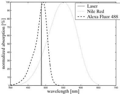
A high resolution progressive scan camera (Basler A113P, Basler (1998)) is used to record the images. It employs a CCD sensor chip with a resolution of 1300× 1030 pixels providing features like electronic exposure time control and partial scan, which can be controlled by the connected PC. Thereby the exposure time is adjusted continously in steps of 20 ms (the scanning duration of the laser beam) to obtain maximum signal-to-noise ratio and the scan area on the CCD chip is adapted to the geometry of the flow cell. In horizontal flow, a partial scan area of 1300 × 600 pixels is used, resulting in a resolution of circa 70 µm in x- and y-direction. Optical bandpass filters (550± 20 nm and/or 600 ±20 nm, the transmittance curves are shown in figure 3.11) are used to limit the imaging to these emission wavelengths of the fluorescent dye, where the refractive indices are closely matched (see chapter 4), and also to screen scattered light e.g. from imbedded air bubbles. In two-phase flow, where two dyes with different emission wavelengths are used, a PC-controlled filter wheel (see figures 3.1

(31)

3.3. EXPERIMENTAL SETUP

Figure 3.2: Photograph of the experimental setup corresponding to ﬁgure 3.1.

and 3.2) is deployed to change between the two ﬁlters. The switch is done after each complete volume scan.

3.3.2 Light source and optics

The light source for illumination is an argon ion laser (Spectra-Physics Stabilite 2017) oper- ating at 488 nm with an output of 1.5 W. The beam is coupled to an optical fiber and then focused on the flow cell to a diameter between 0.5 and 1 mm. It is expanded to a vertical sheet by reflection on the mirror of a galvanometer scanner oscillating at 50 Hz.

3.3.3 Personal computer

The personal computer, equipped with a 500 MHz Intel pentium 3 processor and 1GB RAM, is the central control unit of the measurement setup. It drives the translation stage and the filter wheel via a ISA stepper motor card (Owis SM30). Synchronously it sets the camera parameters (exposure time, partial scan area, gain and offset) and triggers the readout of the CCD via the RS 232 interface. The camera transfers an 8 bit video data stream to a FPGA framegrabber (Silicon Software microenable equipped with a Xilinx XC4085XLA), which is received by the PC at its PCI interface and stored to a hard disk. For a representative experiment (90 images à 1300 × 600 pixel every 30 s) the averaged data rate is circa 2.3 MB/s.

(32)

Mirror

Laser sheet Inlet area

Outlet area

Porous medium

Dye injection

Tube to pump Tube to pump

a

Laser sheet Liquid area

Liquid area Porous medium Tube to pump

Tube to pump

b

Figure 3.3: Flow cells for ahorizontal and b vertical ﬂow.

3.3.4 Translation stage

For the displacement of the mounting plate and the devices mounted on it a motorized translation stage (Owis VTM 80) was employed. Its 2-phase stepping motor performs at a maximum traverse speed of 8 mm/s over a maximum distance of 300 mm. The resolution is speciﬁed as 2.5µm and the repeatability as 10 µm, which is adequate for increments of 400 µm used in the experiments. In a typical experiment 90 parallel planes have been recorded every 30 seconds. During the ﬁrst 14 seconds the actual scanning and data aquisition take place whereas the remaining 16 seconds are used to drive back the translation stage and store the data to the harddisk.

3.3.5 Flow cells

The flow cells are rectangular parallelepipeds made of plexiglass. The solid granulate material is clamped between two metal grids which adjoin to liquid-filled inlet and outlet areas. A tubing pump conveys the fluids through a tube from the outlet to the inlet with adjustable flow rate and direction. Two versions of the flow cells for horizontal and vertical flow direction are sketched in figure 3.3.

The vertical flow cell is mainly used for two-phase flow experiments, like imbibition or drainage processes, where the two liquids have significantly different densities. Its volume for the porous matrix, which is penetrated by a laterally entering laser sheet, has a size of 5×

(33)

3.4. SOLID PROPERTIES 10×5 cm³. The tubing pump is directly connected to the lower liquid area, so that its flow rate is directly coupled to the average liquid velocity in the porous medium. A sketch of the vertical flow cell is shown in figure 3.3b and a photograph is shown in figure 3.4.

The horizontal flow cell is employed for single-phase flow experiments, where the liquid density throughout the medium is approximately constant. The volume of the porous matrix is sized 8×4×4 cm³. Here the liquid is not pumped directly through the porous medium but from and into two containers mounted above the outlet and inlet area, so that the hydraulic heads in these containers reach an equilibrium according to the flow rate given by the pump.

The hydraulic heads can be calculated from the heights of the liquid levels in the containers in order to determine the hydraulic conductivity of the porous medium. The upper coverage of the cell has a hole with a set-in piece of rubber, through which an injection containing dyed liquid is introduced at the beginning of an experiment and the desired quantity of dye is injected. Since the cell is not laterally accessible for the laser sheet, it is placed upon a mirror mounted at 45^◦ so that the laser sheet enters the cell from the bottom. The layout of the horizontal flow cell is shown in figure 3.3a and figure 3.5 shows a corresponding photograph.

3.4 Solid properties

For the solid constituting the porous matrix, a transparent, rigid and inert material is required. Because the number of suitable liquids decreases rapidly with increasing refractive index, the refractive index of the solid should be as low as possible. The two classes of applicable materials are plastics and glasses. Since the refractive index should not depend on the orientation of the grains, which would be the case for birefringent materials, no crystalline but only amorphous materials can come into consideration. The refractive indices of plastics are in a range from 1.49 (acrylic, e.g. Plexiglass or Perspex) to 1.58 (polycarbonate, e.g. Lexan or Makrolon), those of optical glasses from 1.46 (fused silica) to 1.87 (Schott LaSFN9). Since one aim of the present work was to investigate the influence of different surface properties (e.g. contact angle or adsorption rate), one material of each class was used, Plexiglass and fused silica. The refractive index of a solid is a function of temperature and wavelength, which is quantified for the two materials in table 3.1 and figure 3.6. The dependence on the wavelength is used for the precise matching of the refractive indices of solids and liquids as described in chapter 4. The two solids further differ significantly regarding their densities and water/air contact angles as specified in table 3.1. Whereas plexiglass is only moderately acid resistant, fused silica is extremely resistant owing to the very strong silicon-oxygen bonds.

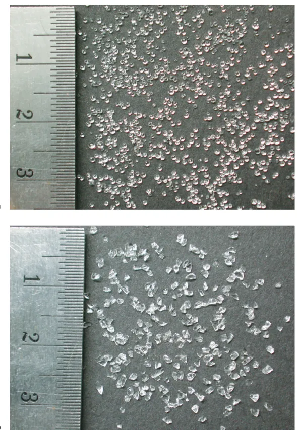
The fused silica was delivered by the manufacturer (Schott Lithotec) as blocks with di- ameters of a few centimeters. They were crushed making use of a jaw crusher which allowed the adjustment of the gap size that the crushed material must pass before leaving. However, the resulting size distribution proved to be very broad and therefore the outcome was further sieved to sizes of 0.6 - 1 mm. The result is shown in ﬁgure 3.7b.

The plexiglass was obtained from the manufacturer (Goodfellow GmbH) in a granulation of 0.6 mm mean diameter. Unfortunately, a big portion of the grains had air bubbles included, which make them unusable for the present application. The separation of the pure grains was performed by immersing them into a NaCl solution with density hardly smaller than that of plexiglass, where the pure grains accumulated at the bottom.

The shape of the grains diﬀers signiﬁcantly for the two materials. Whereas the fused silica grains have many sharp edges, the shape of the plexiglass is close to spherical as shown in

(34)

Figure 3.4: Photograph of the vertical flow cell sketched in figure 3.3b. In the present experiment the oil (marked with an orange fluoresceing dye) in the upper part is displaced by water (marked with a green fluoresceing dye) which is injected from the bottom of the cell.

The distribution of the two liquids is visible in the section illuminated by the laser sheet.

(35)

3.4. SOLID PROPERTIES

Figure 3.5: Photograph of the horizontal flow cell sketched in figure 3.3a. The volume with the porous matrix and the liquid containers are filled with silicone oil, and the injection with the dyed, orange fluoresceing oil is introduced from the top.

(36)

refractive dn/dT density water/air mean porosity Solid

index n [^◦C⁻¹] ρ[g/cm³] contact angle diameter ¯d φ[cm³/cm³] Fused silica 1.46^a 9.8·10^−6a 2.2^a ≈0^b 0.8 mm 0.48 Plexiglass 1.495^c −105·10^−6c 1.19^d 59.3^b 0.6 mm 0.37

Table 3.1: Properties of solids for use as the porous matrix.

afrom Schott (2001) atT = 20^◦C andλ= 588nm

bfrom Adamson (1997)

cfrom Waxleret al.(1979) atλ= 589nm

dfrom Goodfellow (1999)

300 400 500 600 700

1.44 1.46 1.48 1.5 1.52 1.54 1.56

Fused silica Plexiglass

Silicon oil T=25˚C NaI solution 60% T=25˚C

wavelength [nm]

refractive index

Figure 3.6: Refractive index as a function of wavelength for fused silica (from Schott (2001)), plexiglass (from Waxler et al. (1979)), silicone oil (from Cargille (1999)) and sodium iodide aqueous solution (from Narrowet al. (2000)).

figure 3.7a. In contrast to the plexiglass grains, the fused silica grains are considerably oblate, which is hardly visible from figure 3.7b since they are mostly lying on the flat side. These differences in grain morphology and size distribution effectuate the different porosity values given in table 3.1. They were calculated from the weight of a predefined volumeV filled with the porous media and their respective densities:

φ= 1− m_solid

ρsolidV. (3.1)

3.5 Liquid properties

For the present technique two immiscible and transparent liquids matching the refractive index of the solids are required. Additionally they are demanded to be inert, nontoxic, nonvolatile

(37)

3.5. LIQUID PROPERTIES

a

b

Figure 3.7: Granular materials for use as transparent porous matrix: a plexiglass b fused silica. The numbers on the ruler denote centimeter.