General Relativity
by Benjamin Bahr
Typed by Claudia Sch¨ onberg
Contents
1 Special Relativity 3
1.0.1 From Galilei to Lorentz . . . 4
1.0.2 Minkowski space . . . 6
1.1 Minkowski-distance squared . . . 8
1.2 Change of inertial systems . . . 10
1.2.1 Relativistic kinematics . . . 16
1.2.2 Non-inertial observers. . . 18
1.3 The gravitational force and relativity . . . 24
1.3.1 Movement of an inertial observer in a gravitational field . . . 27
2 Tensor fields on arbitrary manifolds 31 2.1 Vectors, dual vectors and tensors . . . 31
2.1.1 Vectors . . . 31
2.1.2 Dual vectors . . . 32
2.1.3 Higher order tensors . . . 33
2.1.4 Some physical examples . . . 34
2.1.5 Operations on tensors. . . 36
2.1.6 Symmetries of tensors . . . 37
2.2 Manifolds . . . 39
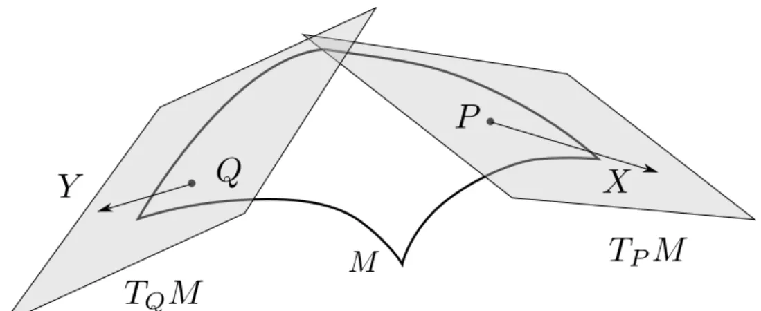
2.2.1 Tangent vectors . . . 40
2.2.2 Basis forTpM . . . 42
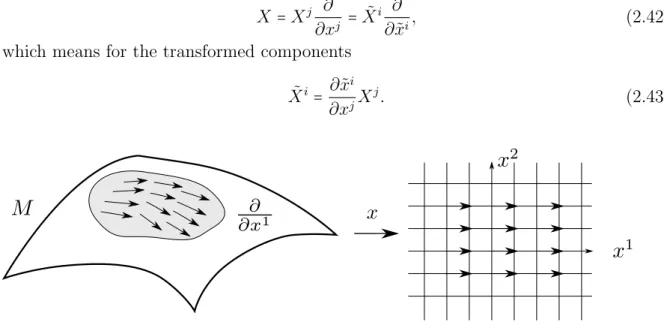
2.2.3 Vector fields . . . 43
2.2.4 1-forms . . . 44
2.2.5 Curve integrals of 1-forms . . . 44
2.2.6 General tensor fields onM . . . 45
2.2.7 The Cartan derivative . . . 45
2.3 Metrics, connections and curvature . . . 46
2.3.1 The covariant derivative . . . 47
2.3.2 Geodesics . . . 54
2.3.3 Parallel transport . . . 56
2.3.4 Geometric interpretation of torsion. . . 58
2.3.5 Curvature. . . 60
2.3.6 Symmetries of the Riemann curvature tensor. . . 63
2.3.7 Independent components ofRklmn . . . 64
3 General Relativity 66 3.1 Fermi normal coordinates . . . 67
3.1.1 Curvature and tidal forces . . . 71
3.2 Dynamics of general realtivity . . . 75
3.2.1 The energy-momentum tensor. . . 75
3.2.2 Connection betweenTµν and gµν . . . 77
3.2.3 The Einstein equations and non-uniqueness of solutions . . . 82
3.2.4 The Einstein-Hilbert action . . . 84
4 Applications of General Relativity 89 4.1 Killing vector fields . . . 89
4.2 The Schwarzschild metric . . . 91
4.3 Interior solution of Einstein’s equations . . . 95
4.3.1 The Kruskal extension . . . 101
4.4 Gravitational red-shift . . . 104
4.5 Motion in rotationally symmetric gravity field . . . 107
4.5.1 The massive case: =1 . . . 109
4.5.2 The massless case: =0 . . . 110
4.5.3 Light scattering . . . 111
4.6 Cosmology . . . 114
4.6.1 Homogeneous and isotropic matter . . . 117
4.6.2 Light propagation in FRW spacetimes . . . 120
4.7 Linearised solutions and gravitational waves . . . 128
4.7.1 Linearised gauge transformations . . . 129
4.7.2 Gravitational waves . . . 130
4.7.3 Polarisations of gravitational waves . . . 132
1 Special Relativity
From 1687 until the beginning of the 20th century, Newton’s notion of absolute space and time were the de-facto standard for physical theories describing mechanical motion of point particles and extended objects. It is so pervasive of the realm of physics, and in accordance with our everyday experiences, that it is still the foundation of most courses in physics and engineering. The equations for building ships, shooting rockets, up to the movement of stars and planets, rested on the foundation of Newton’s three laws of mechanics, as well was the law of gravity.
It was just in 1887, when it turned out that Newtonian notions of space and time, together with the well-known Galilei-transformation, had to be extended to describe velocities close to the speed of light. In thie first chapter, we will go over this generali- sation.
First we recall Newton’s notions of space and time, as well as that of inertial observers and Galilei-transformations.
In Newtonian physics, space has the form of a 3-dimensional affine space, while time has the structure of a 1-dimensional affine space, i.e. a line. An inertial observer is one on whom no physical forces act. Such an observer moves, as per Newton’s first law of mechanics, either not at all, or along a straight line with constant velocity.
To each inertial observer O corresponds an associated inertial coordinate system, with coordinates xi, where i=1,2,3. In these coordinates, Newton’s second law can be expressed as
d2xi dt = 0
for any curve t ↦xi(t) of an inertial observer. Of course, every inertial observer is at rest in their worn inertial coordinate system, namely at the originxi=0.
All inertial observers are considered equivalent, so it is prudent to understand how the coordinates of one inertial observer can be transformed into those of another one.
Assume there are two inertial observers O and ˜O, with respective coordinates xi and
˜
xi. From ˜O’s perspective, O moves in positive ˜x1-direction with velocity v. If the axes of the two coordinate systems are parallel, then the two sets of coordinates are related by the Galilei transformation law
˜t = t
˜
x1 = x1 + vt
˜ x2 = x2
˜ x3 = x3
(1.1)
Heret and ˜t are the time measured by either observer, which agree, since time is inde- pendent of the observer. Assume that at t =0, observer O throws a stone in positive x1-direction with velocitydx1/dt=w. Then ˜O would measure the velocity of that stone to be
˜
w = d˜x1
d˜t = d˜x1
dt = dx1
dt +v = w+v. (1.2)
So velocities add up in Newtonian mechanics, which is what conforms to our everyday experience.
1.0.1 From Galilei to Lorentz
In 1887, Michelson and Morley attempted to measure the relative speed of the Earth with respect to the aether, which at that time was thought to be the medium in which electromagnetic waves propagate. The experiment, famously, turned out to have a neg- ative result: No matter in which direction the measurement apparatus moved, it always measured a speed pf
c = 3⋅108ms−1.
This directly contradicts (1.2), which predicts that two differently moving observers should measure different speeds of light, differing by their relative difference in velocity.
But they did not. As it turned out, every inertial observer measures the same value of the speed of light, directly contradicting the Galilei transformations. A way out was proposed by slightly changing the transformation laws (1.1).
As it turns out, the timethas to be transformed along side the other three coordinates xi. To treat them all on the same footing, one introduces
x0 ∶= ct.
The collection of four coordinates are being denoted byxµ, withµ=0,1,2,3. The ansatz for the new transformation can be written as
˜
x0 = A(x0 +Bx1)
˜
x1 = C(x1 +vt) = C(x1 +βx0)
˜ x2 = x2
˜ x3 = x3 with β∶= vc.
Now assume that at time t = 0, O sends out a light ray in the x1-direction. The coordinates on the light rays then satisfydx1/dt=c, so x1=x0, or, more general,
(x0)2 − (x1)2 − (x2)2 − (x3)2 = 0. (1.3)
To conform with the result from Michelsons and Morleys experiment, we have to demand that the curve on ˜O’s system satisfies the same equation, just for the ˜xµ. From this it follows that
0 = (x˜0)2 − (x˜1)2 − (x˜2)2 − (x˜3)2
= A2(x0−Bx1)2 −C2(x1 − v
cx0)2 − (x2)2 − (x3)2
= (A2−C2v2
c2) (x0)2 − (C2−A2B2) (x1)2 − (x2)2 − (x3)2 + (2Cv
c −2AB)x0x1. From comparison with (1.3) we can read off that
A2−C2v2
c2 = 1, (1.4)
C2−A2B2 = 1, (1.5)
2Cv
c−2AB = 0. (1.6)
This can be solved forA,B, andC, and we obtain1 B = β = v
c, A = C =∶ 1
√1−β2 γ.
which gives us the formula for the Lorentz transformation as
˜
x0 = γ(x0+βx1),
˜
x1 = γ(x1 + βx0),
˜
x2 = x2,
˜
x3 = x3.
(1.7)
This transformation law is an example of a Lorentz transformation, which are those affine coordinate transformations which preserve the speed of light for all inertial observers.
To check how the law (1.2) changes in this case, consider the same situation as before, but now ˜O’s coordinates are related to O’s via (1.7) and not (1.1). One gets, for the
1Up to signs, which would correspond to a parity transformation, or time reflection in ˜O’s system.
These are allowed, but not the solutions we look at here.
time
space
event: two stars collide expanding shock wave
Figure 1.1: In a space-time diagram, times increases upwards, so a diagram of two stars encircling each other, colliding and exploding would roughly look like this.
speed measured in ˜O’s system, that
˜
w = d˜x1
d˜t = cd˜x1
d˜x0 = c(d˜x0 dx0)−
1d˜x1 dx0
= c( d
dx0(γ(x0+βx1)))−1 d
dx0 (γ(x1+βx0))
= c
1+βwc(w
c +β) = v + w 1+vwc2
For speeds small w.r.t. the speed of light, i.e.¨uv, w ≪c; this tends towards (1.2), while forw=cthis leads to ˜w=c, as demanded.
1.0.2 Minkowski space
A consequence of replacing Galilei- with Lorentz transformations is not just an adapta- tion of formulas, but a reworking of Newton’s notion of space and time. In particular, one considers a four dimensional unification of space and time (the so calledMinkowski space R1,3). Curves in Minkowski space describe motions, e.g. two stars circling each other and colliding. A point in Minkowski space is called an event (when and where something happens). In the coordinate system in Minkowski space, the point 0 is the origin event. The coordinate axes are x0 =ct, x1 =x, x2 =y, x3 =z. We interpret this as follows: The parameter t is the elapsed time as measured by someone sitting at x1 = x2 = x3 = 0 with the conversion factor c which works because c is the same in all frames of reference. Thexi,i=1,2,3 are the distance from the x0-axis. We write xµfor a four vector. In our convention, Greek indices will always run from 0 to 3.
The curve that an object (observer, space ship...) traces out in Minkowski space is called aworld line. A world line is a map
φ↦xµ(φ) (1.8)
with a more or less arbitrary curve parameterφ.
Aninertial system is defined as a coordinate system that has the following properties:
"world line"
Figure 1.2: The world line of a (point-like) object, traced out in a coordinate system.
Any freely moving object (i.e. one without force acting on it) is described by a straight line.
Light rays always move on world lines with slope equal to 1.
The first condition is similar the old Newtonian physics: A coordinate system is called
”inertial” if and only if F⃗ =mx¨⃗ holds, i.e. ¨x⃗=0 for freely moving objects.
The second condition means that the speed of light is the same in all inertial systems.
To each inertial observer corresponds an inertial system. The world line of the observer in his own frame of reference is given by
xµ(t) =
⎛⎜⎜
⎜⎝ ct
0 0 0
⎞⎟⎟
⎟⎠
. (1.9)
at rest (in this CS)
slower than light
faster than light
Figure 1.3: World lines of point particles moving freely. The slope of the line indicates how fast the particle moves.
1.1 Minkowski-distance squared
In Minkowski space, the distance between two points does not exist, but the distance squared does:
d(E1, E2)2∶=c2(∆t)2− (∆x1)2− (∆x2)2− (∆x3)2= ∑3
µ,ν=0
ηµν∆xµ∆xν (1.10) with the Minkowski metric
η=
⎛⎜⎜
⎜⎝
1 0 0 0
0 −1 0 0 0 0 −1 0
0 0 0 −1
⎞⎟⎟
⎟⎠
. (1.11)
Figure 1.4: Two events E1 and E2 in Minkowski space.
From now on we want to save space and omit the sum over indices. Whenever there is an index appearing twice (once as upper, once as lower index), it is summed over. This is called theEinstein convention. Now, we can write
d(E1, E2)2=ηµν∆xµ∆xν. (1.12) Also, if an index appears only once (called afree index), it has to appear on both sides of the equation, and in the same position. An index is not allowed to appear more than twice. See table 1.1 for examples.
The Minkowski squared distance can have either sign, which is why d(E1, E2) doesn’t exist. We categorize the distances squared by their sign:
d(E1, E2)2>0: time-like
d(E1, E2)2<0: space-like
d(E1, E2)2=0: light-like
allowed not allowed xµ=yµ xµ=yµ
xµ=Tνσµνxσ+yµ xµ=yν
ηµνxµxν =3 xµyν =Tµν+ηµν xµyν =Tµν xµ=ηνσyσzσTσνµ
Table 1.1: Allowed and disallowed index placements Velocity vectors of curves have a Minkowski length squared:
∣dxµ
dφ∣2 =ηµν
dxµ dφ
dxν
dφ. (1.13)
The velocity vector does not express the velocity directly, the velocity is the inverse slope of dxµ/dφ. A curve is called time-like/space-like/light-like if ∣dxµ/dφ∣2 >0/ <0/ = 0∀φ. The Minkowski length of a time-like curve with [0,1] ∋φ↦xµ(φ) is given by
l(x) = ∫01dφ
¿Á ÁÀ∣dxµ
dφ ∣2. (1.14)
This lengthl(x) does not depend on the parameterization of x. Here, x is the complete world line, while xµ describes its components.
Figure 1.5: Velocity vector of a world line.
We assume that no physical signal can travel faster than light. So an event E can not have an influence on all other events E′, not even all of those which, in an inertial system, have a larger x0-coordinate (i.e. lie in the future of E). In fact, for two events E, E′, which are space-like with respect to each other, different inertial observes can disagree on which of the two happens before the other!
Because of this, it is convenient to define “future” and “past” in a coordinate-independent way. First of all, we call a curve φ → xµ(φ) causal, if ∣dxµ/dφ∣2 ≥ 0. We call it future pointing if dx0/dφ>0, andpast-pointing if dx0/dφ<0.
For an event E, the setJ+(E)of all eventsE′ which are in thecausal future of E are those which can be reached fromE by a future-pointing, causal curve, i.e.:
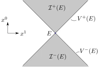
J+(E) ∶= {E′∣there is a future pointing, causal curve from E to E′} (1.15) Similarly, J−(E), the causal past of E, is the set of all events with a causal, future pointing curve from E′ to E, or alternatively, a causal past-pointing curve from E to E′. The chronological future/past I±(E) consist those events E′, which can be reached fromE by a future-(past-pointing time-like curve. The light-cone of E, denoted VE, is given by all eventsE′ that can be reached by alight signal from E, i.e.
V ∶= {E′∣d(E, E′)2=0}. (1.16) The future / past light cone V± is defined as one would expect (see figure1.6).
Figure 1.6: Chronological future and past of an eventE. Here,J+(E) = I+(E)∪V+(E), similarly for x↔ −.
1.2 Change of inertial systems
Let the coordinates of an event in one inertial system be calledxµand in another inertial system ˜xµ. How are they related?
Remember: Free particles move along straight lines. That means the transformation law has to be affine-linear. An affine transformation conserves points, straight lines and planes. The transformation law should look something like this:
yµ=Λµνxν +aµ. (1.17)
Here, Λµν is a 4×4 matrix which does not depend on x. The upper index labels the rows, the lower index the columns. The vector aµ is a translation independent of x. It
can be arbitrary, the interesting question is what forms Λ can take.
Figure 1.7: Two inertial systems, describing Minkowski space. The same event E has coordinates x0 =4,x1 =3, and ˜x0 =1, ˜x1=1.
The speed of light is the same in all inertial systems. If d(E1, E2)2 = 0 in one iner- tial system, it has to be 0 in all inertial systems. In fact, one can show that, if two observers use the same scale of measurement, and use only light signals to construct their coordinate systems, they will always agree on the value d(E1, E2)2 between two events E1, E2. So we shall demand to only allow coordinate transformations that leave d(E1, E2)2 unchanged. Label the coordinates of the events in one inertial system xµand yµ, in the other inertial system ˜xµ and ˜yµ. Then the length squared in the first system is
dIS1(E1, E2)2=ηµν(xµ−yµ)(xν−yν)
=! dIS2(E1, E2)2
=ηµν(x˜µ−y˜µ)(x˜ν−y˜ν)
=ηµνΛµσΛνρ(xσ−yσ)(xρ−yρ)
=ησρΛσµΛρν(xµ−yµ)(xν−yν). (1.18) Here, we used the same ηµν and in the last step, simply renamed the indices that are summed over. This equation holds for all events E1, E2, i.e. all coordinates xµ, yµ. It follows that
ηµν =! ησρΛσµΛρν. (1.19) The Lorentz-transformations in matrix form are
ΛTηΛ=η. (1.20)
They form the Lorentz group, which is the group
L =O(1,3) = {Λ∈R4×4∣ΛTηΛ=η}. (1.21)
The group O(n) is the group of orthogonal n×n matrices, meaning its elements are matrices that are real and whose inverse is equal to their transpose. The group is called the orthogonal group.
Important members ofO(1,3) are
rotations in space:
Λ=
⎛⎜⎜
⎜⎝
1 0 0 0
0
0 R
0
⎞⎟⎟
⎟⎠
(1.22) with a rotation matrix
R∈SO(3) = {R∈R3×3∣RTR=1,detR=1}. (1.23) The groupSO(n)is called thespecial orthogonal group and is a subgroup ofO(n). It contains all elements of O(n) with determinant equal to 1. These matrices de- scribe rotations, which is why the group sometimes is called the rotation group.
boosts that connect two inertial systems for observers with constant velocity with respect to each other. A boost in x1-direction has the form
Λ=
⎛⎜⎜
⎜⎝
coshψ −sinhψ
−sinhψ coshψ 1
1
⎞⎟⎟
⎟⎠
(1.24)
with ψ∈R.
further elements: Time reversal
Tµν =
⎛⎜⎜
⎜⎝
−1 1
1 1
⎞⎟⎟
⎟⎠
(1.25)
and parity (reversal of spatial orientation)
Pµν =
⎛⎜⎜
⎜⎝ 1
−1
−1
−1
⎞⎟⎟
⎟⎠
. (1.26)
Warning: Even though p and η look exactly alike, they are not identical! This is already apparent from their index positions (η has two indices downstairs, P one up- and one downstairs), but also from their respective role: ηis used to construct the Minkowski distance between events, while P is a coordinate transformation, i.e. it is a way to compute one set of coordinates of an event, from its coordinates in another coordinate system.
Time dilation
In each inertial system for each observer, the coordinates are what the observer at rest would measure with rods and clocks. In particular, to each inertial system corresponds one inertial observer, and vice versa. In the future, we will use them interchangeably.
2 From the coordinate x0 = ct, t = x0/c is the time that passed for the observer, the other three are the distance from the observer, along the three main axes. In Minkowski space, all points that have the same t-coordinate form a plane of simultaneous events.
In equation ??, we already calculated how the world lines of two observers look in the same system. Now assume that at 0, they meet and synchronize their clocks. I.e., in IS1, O1 is at rest and O2 moves in negative x1-direction with speed v. At the event where they meet, both clocks show t =s = 0. At t = t0, O1 looks at his clock and asks what O2’s clock shows at this moment. The event E is “the position of O2 at t=t0”. In IS1, E has the coordinates(ct0,−vt0,0,0)T with v=ctanhψ. Transform this to IS2:
⎛⎜⎜
⎜⎝
coshψ sinhψ sinhψ coshψ
1 1
⎞⎟⎟
⎟⎠
⎛⎜⎜
⎜⎝
ct0
−ct0tanhψ 0 0
⎞⎟⎟
⎟⎠
=
⎛⎜⎜
⎜⎜⎝
ct0(coshψ−sinhcosh2ψψ) 0
0 0
⎞⎟⎟
⎟⎟⎠
=
⎛⎜⎜
⎜⎝
ct0
coshψ
0 0 0
⎞⎟⎟
⎟⎠
. (1.27)
The x1 coordinate of E is 0 because O2 hasn’t moved in this system. In the second line, the identity cosh2ψ−sinh2ψ=1 was used. This factor of coshψ depends on v the following way:
coshψ =
¿Á
ÁÀ cosh2ψ cosh2ψ−sinh2ψ
= 1
√1−tanh2ψ
= 1
√1−v2/c2
=∶γ.
Since v≤c, the expression coshψ1 is always smaller or equal to 1. So the event E has, in IS2, the coordinates (ct0√
1−v2/c2,0,0,0)T. That means that for O1, it seems like less time has passed for O2 by a factor of √
1−v2/c2.
2In fact, in the classical literature about relativity, much time is devoted to the technical aspects of how an inertial observer would construct their inertial coordinate system, with light signals being sent back and forth.
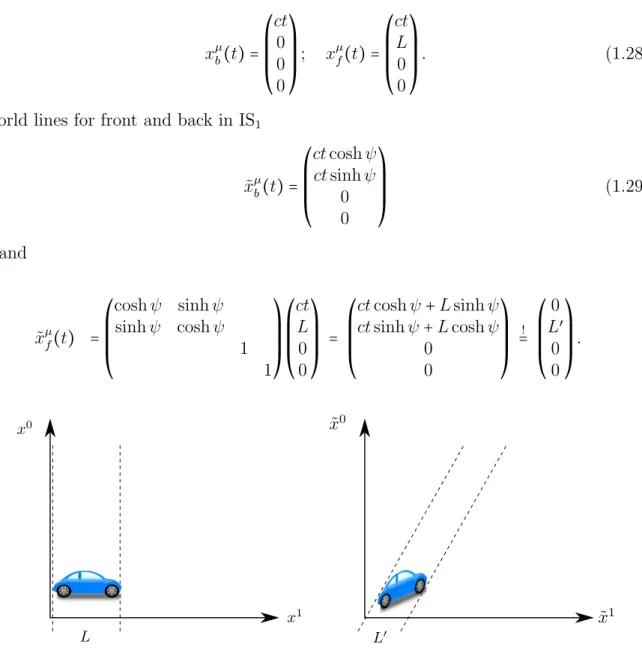
Length contraction
O1 sits in a car of length L and passes O2 with speedv. The front and the back of the car have the following coordinates:
xµb(t) =
⎛⎜⎜
⎜⎝ ct
0 0 0
⎞⎟⎟
⎟⎠
; xµf(t) =
⎛⎜⎜
⎜⎝ ct L 0 0
⎞⎟⎟
⎟⎠
. (1.28)
World lines for front and back in IS1
˜ xµb(t) =
⎛⎜⎜
⎜⎝
ctcoshψ ctsinhψ
0 0
⎞⎟⎟
⎟⎠
(1.29)
and
˜
xµf(t) =
⎛⎜⎜
⎜⎝
coshψ sinhψ sinhψ coshψ
1 1
⎞⎟⎟
⎟⎠
⎛⎜⎜
⎜⎝ ct L 0 0
⎞⎟⎟
⎟⎠
=
⎛⎜⎜
⎜⎝
ctcoshψ+Lsinhψ ctsinhψ+Lcoshψ
0 0
⎞⎟⎟
⎟⎠
=!
⎛⎜⎜
⎜⎝ 0 L′
0 0
⎞⎟⎟
⎟⎠ .
Figure 1.8: A car at rest in coordinates xµ, and moving with constant speed v in coor- dinates ˜xµ.
The way for O2 to determine the lengthL′in their coordinate system is to ask “what is the ˜x1-component of the world line of the front of the car, at that moment when the back of the car passes my position?” To compute this, one needs to compute the intersection of ˜xµf(t) with the ˜x1-axis. Let us assume that happens at the curve parameter t=t0, so
ct0= −Ltanhψ= −Lv
c (1.30)
and
L′ = ct0sinhψ+Lcoshψ = −Ltanhψsinhψ+Lcoshψ
= L(−sinh2ψ
coshψ +cosh2ψ
coshψ ) = L
coshψ = L γ. The car appears shorter for O2 by a factor of √
1−v2/c2. Elapsed time of a moving observer
How much time passes for an observer moving along an arbitrary (not necessarily straight) world line x between events E1 = x(0) and E2 = x(1)? To calculate this, we subdivide the interval[0,1] into small bits:
0=φ0 ≤φ1≤φ2≤...≤φN =1. (1.31) On the segment between xµ(φj)and xµ(φj+1), the curve is nearly linear (if the curve is smooth). We transform to the system in which the observer is at rest (for this moment):
˜
(j)xµ
1 =Λ(j)µνxν(φj) +aµj =
⎛⎜⎜
⎜⎝ 0 0 0 0
⎞⎟⎟
⎟⎠
(1.32)
˜
(j)xµ
2 =Λ(j)µνxν(φj+1) +aµj =
⎛⎜⎜
⎜⎝ c∆tj
0 0 0
⎞⎟⎟
⎟⎠
. (1.33)
The elapsed time is
∆tj =
√
d((j)x˜1,(j)x˜2)2
c . (1.34)
The Minkowski distance squared is invariant under Lorentz transformations, which means that
∆tj =√
d(xµ(φj), xµ(φj+1))2 =1 c
√ηµν(xµ(φj+1) −xµ(φj))(xν(φj+1) −xν(φj)). (1.35)
Use the approximation
xµ(φj+1) ≈xµ(φj) +dxµ
dφj∆φj + O(∆φ2j) (1.36) to obtain
∆tj ≈1 c
√
ηµνdxµ dφ
dxν
dφ∆φj + O(∆φ2j). (1.37)
Figure 1.9: Approximation of a curve with short straight lines.
The total elapsed time is the sum over all intervals of time:
T = lim
N→∞
N−1
∑
i=0
∆tj= 1 c∫
1 0
dφ
¿Á ÁÀ∣dxµ
dφ∣2= 1
cl(x). (1.38) Timelike curves in Minkowski space can be parameterized by theproper time (Minkowski length):
s(φ) = ∫φφ
0
dφ′
¿Á ÁÀ∣dxµ
dφ′∣2. (1.39)
The curve is regular, when dxµ/dφ′ /= 0 holds for all φ′. The relation can be inverted as s↦φ(s), so that we can write
ˆ
xµ(s) ∶=xµ(φ(s)). (1.40) The length of the curve is given by
l(xˆ) = ∫ss1
0
ds=s1−s0 (1.41)
whereds is called theinfinitesimal line element. It is given by
ds2=c2(dt)2− (dx1)2− (dx2)2− (dx3)2=ηµνdxµdxν. (1.42) It contains all information about the spacetime geometry and tells how much time passes for an observer that moves through spacetime.
1.2.1 Relativistic kinematics
Observers in special relativity move along world lines, usually parameterised by proper time s↦xµ(s). The 4-velocity for a particle that is obtained by deriving with respect to proper time is given by
uµ ∶= cdxµ ds .
Note that the vector u has the dimension of a velocity. It satisfies u2 ∶= ηµνuµuν = c2. The 3-velocity measured by the inertial observer who belongs to the coordinate system isv, which has components⃗ vi with i=1,2,3, given by
vi ∶= dxi
dt = cdxi
dx0. (1.43)
Note that the proper times (time passing for the particle) and x0 (time passing for the inertial observer) do not run at the same speed, there is a difference
ds = 1 γdx0 coming from time-dilation. Hereγ is the factor
γ = 1
√ 1−v⃗c22,
where ⃗v is the velocity (1.43). Note that, for a general, accelerated world line, this will depend on s. With this we get
uµ = cd
dsxµ = γc d dx0xµ. Sou is the vector with components
u = γ(c,v⃗).
For relativistic kinematics, an important physical quantity is the so-called 4-momentum pof a particle, which is defined by
pµ ∶= m0uµ.
Herem0 is the so-called rest mass, which is the inertial mass measured in the rest frame of the particle. Note thatm0 is the same in every inertial system by definition, while the inertial mass (i.e. the “resistance” of a particle against being accelerated) might depend on the frame. One also writes
p = (γm0c, γm0⃗v) =∶ (mrelc, mrel⃗v).
mrel ∶= m0γ is called the “relativistic mass”. It captures the inertial properties of the particle. Note that the 0-component of pµ, divided by c, has dimensions of an energy, and indeed one writes
p = (E/c, p⃗). The one has
p2 ∶= ηµνpµpν = E2 c2 − ⃗p2
while on the other hand, one hasp2=m20u2=m20c2, so E2 = c2p⃗2 + m20c4. Indeed, for small velocities∣⃗v∣ ≪c, one gets
E = m0c2 + 1
2m0v⃗2 + . . . .
SoE indeed measures the energy stored in a particle, which has both a rest contribution m0c2, as well as a kinetic contribution, which, to lowest order in the velocity, coincides with the non-relativistic kinetic energy.
For interactions between particles, it is the sum of all pµ which is conserved, both in classical relativistic mechanics, as well as in QFT. This incorporates both momentum- and energy conservation in physical processes. Mechanical laws are, as in Newtonian mechanics, written in the form
d
dspµ = fµ,
where fµ is the relativistic analogue of a force. The precise form of the force depends on the physical theory at hand.
1.2.2 Non-inertial observers
So far, we have only considered inertial observers, which means coordinate systems of observers moving freely. But in reality, observers are often non-inertial (accelerated) because they are subject to forces (electromagnetism, gravity, ...). The coordinate sys- tems of those observers will not be inertial. Because of that, there will beinertial forces.
Those are forces that arise in non-inertial reference frames due to their acceleration and seem to have no physical origin, for example centrifugal forces in rotating frames. Be- cause of this, they are often also called pseudo forces.
Consider an observer O moving along the world line
xµ(s) =
⎛⎜⎜
⎜⎝
dsinhds dcoshds
0 0
⎞⎟⎟
⎟⎠
(1.44)
that is parameterized by the proper time s. Construct a coordinate system with coor- dinatesyµ for O. This will not be an inertial system!
Between the proper times ands+∆s, the observer nearly moves along a straight line (if ∆s≪1):
xµ(s+∆s) =xµ(s) +dxµ
ds ∆s+ O(∆s2) (1.45)
where we encounter the proper velocitydxµ/ds. This means that for a short time interval, O is moving almost along the same world line as the inertial observer OI with world line
xµ(I)(τ) =xµ(s) +dxµ
ds dτ (1.46)
world line of O
Figure 1.10: World line of the Rindler observer1.44.
withτ being the proper time of OI. So at least for this short moment, O and OI should see the world (nearly) the same way, so they should have the same plane of simultaneous events (at least in their near vicinity) which is given by
Σs= {xµ(s) +Xµ∣ηµνXµdxν
ds (s) =0}. (1.47)
It is orthogonal toxµ(I). Having the same plane of simultaneous events means having the same notion of things happening right now.
For this moment, the world line for OI is a straight line tangential to the world line of O at the pointxµ(s) =xµ(I)(0). The vectorXµcomes from the origin and crossesxµ and xµ(s).
Because O is accelerating, Σs and Σs′ will not be parallel for s /= s′. We calculate the proper velocity as
dxµ ds (s) =
⎛⎜⎜
⎜⎝ coshsd sinhsd
0 0
⎞⎟⎟
⎟⎠
(1.48)
(the prefactor d vanished because we get an additional factor 1/d from the derivative).
The directions orthogonal (in the Minkowski inner product) to that are
e(1s)=
⎛⎜⎜
⎜⎝ sinhsd coshsd
0 0
⎞⎟⎟
⎟⎠
, e(2s)=
⎛⎜⎜
⎜⎝ 0 0 1 0
⎞⎟⎟
⎟⎠
, e(3s)=
⎛⎜⎜
⎜⎝ 0 0 0 1
⎞⎟⎟
⎟⎠
. (1.49)
All of these (3d hyper-)planes Σs intersect in {xµ ∶ x0 = x1 = 0, x2, x3 arbitrary} (sinh is only 0 if its argument is 0). At these points, the coordinates yµ break down: The event {xµ =0} would be having several different yµ-coordinates, but coordinates must uniquely define events.
Figure 1.11: Plane of simultaneity Σs for the Rindler observer O at proper time s. It coincides with that of the inertial observer OI.
Coordinate system O is yµ (with y0 = s) such that his world line in his coordinate system is given by
yµ(s) =
⎛⎜⎜
⎜⎝ s 0 0 0
⎞⎟⎟
⎟⎠
. (1.50)
The transformations between the coordinate systems are x0 = (y1+d)sinhy0
d (1.51)
x1 = (y1+d)coshy0
d (1.52)
x2 =y2 (1.53)
x3 =y3. (1.54)
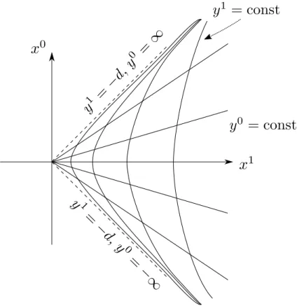
Here we already see that in O’s system, y1 = −d is a problem. If y1 = −d, y2 =y3 = 0, all points for all y0 get mapped to {xµ=0}. Since coordinates need to uniquely identify events, we can only allow y1> −d.
Figure 1.12: Rindler coordinates yµ, covering the Rindler wedge. They break down at the boundary of that wedge.
For y1> −d, the coordinates xµ(yµ)can be inverted:
y0=d⋅arctanhx0
x1 (1.55)
y1=√
(x1)2− (x0)2−d (1.56)
y2=x2 (1.57)
y3=x3. (1.58)
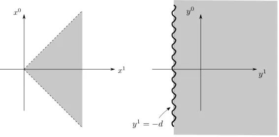
This only works for ∣x1∣ > ∣x0∣, because otherwise, y1 would become imaginary. So we only take x1 > ∣x0∣. This is called the Rindler wedge. In the inertial system, if we only look at the x0, x1-plane, this is only the right area outside of the light cone. In O’s system, it corresponds to a Rindler horizon at y1 = −d where O’s world ends, so to speak.
Figure 1.13: Coordinate patches in the Rindler wedge. In Rindler coordinates, the region y1 ≤ −d is not accessible (“behind the horizon”).
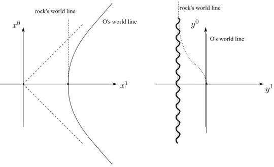
In O’s system, a freely moving observer does not move along a straight line. Assume that O has, in his space ship, a rock. That rock is tossed out of the airlock at s = 0.
From that point on, the rock moves freely. In the inertial system, the world line of rock is given by
xµ(r)(τ) =
⎛⎜⎜
⎜⎝ τ d 0 0
⎞⎟⎟
⎟⎠
, (1.59)
the rock moves on a straight line. In O’s system however, the world line takes the form
yµ(r)(τ)
⎛⎜⎜
⎜⎝
d⋅arctanhτd
√d2−τ2−d 0 0
⎞⎟⎟
⎟⎠
. (1.60)
The rock never crosses the horizon because for the same reasons as before, ∣τ∣ > ∣d∣ is never possible. However,τ approaches d. The rock comes infinitely close to the horizon, but never crosses it.
O's world line
rock's world line rock's world line
O's world line
Figure 1.14: World line of the Rindler observer, and a rock that is being dropped, both in Minkowski coordinates and Rindler coordinates.
For small ∣τ∣ ≪1, we can expandy0(r) and y(1r) in a Taylor expansion:
y(0r)(τ) ≈τ (1.61)
y(1r)(τ) ≈ − 1
2dτ2. (1.62)
We expanded√
d2−x−d≈d−d−2dx +...with x=τ2. Equations 1.61 and 1.62 hold for a short time. Compare this to ”free fall” in a constant gravitational field: The change in height is given by
∆h(t) = −1
2gt2 (1.63)
with the accelerationg.
Forτ →d, y0(τ) → ∞and y1(τ) → −d. This means that the rock can reach the horizon after an infinite amount of time. From O’s point of view, the rock approaches the horizon, but never reaches it. Also, it seems to ”freeze in time”.
The Rindler observer feels a force in negativey1-direction with an acceleration a= − 1
y1−d (1.64)
which diverges at the horizon. The force that this Rindler observer experiences is ”fic- titious” (it has no physical cause, so to speak, like the centrifugal or the Coriolis force).
They are a result of being in a non-inertial system.
1.3 The gravitational force and relativity
Special relativity posed a new framework for the motion of point particles, which was an extension of Newton’s mechanics, in particular his three laws of motion. It also fit perfectly with Maxwell’s electrodynamics, which describes the electric interaction of particles. It was clear pretty quickly, that also Newton’s law of gravity should be adapted to fit into the relativistic framework proposed by Einstein. In particular, the Coulomb potential of a charge at rest and the gravitational potential of a mass at rest both looked fairly similar, so the two forces should be quite similar as well, right?
Unfortunately, writing a law of gravitational attraction between massive particles in a way that fit with Einstein’s special relativity theory proved quite difficult. There were several reasons for that, but one of the major ones was that, although gravity and electro- magnetism might look similar in some way, they were quite different in other important ways. For instance, the electric charge, which is the source for the electromagnetic field, does not change under Lorentz transformations (it is also called aLorentz-scalar), while the mass of a particle, which is the source of the gravitational field, turned out to be dependent of the observer. This proved to be an insurmountable obstacle for writing down a law of gravity which works for relativistic particles in Minkowski space.
However, Einstein found a solution to this problem, in the so-called equivalence prin- ciple. Namely, he realised that an observer falling freely in the gravitational field (e.g. of the Earth), feels weightless during their fall. In Newtonian mechanics, this is a conse- quence of the fact that an observer, who is accelerated by the gravitational field, feels a fictitious force which exactly counteracts the gravitational force. Einstein, however, realised that the freely falling observer themself is an inertial observer, and therefore feels weightless, while the person standing on the surface of the Earth does not feel a physical force, but feels a fictitious force – just like the Rindler observer, who keeps a constant distance to the horizon.
So the equivalence principle states that gravity is equivalent to a fictitious force one feels due to an accelerated motion.
Consider the following four observers observing the fall of an apple:
I The first observer in in a room on earth. The apple is accelerated downwards with
⃗ g.
II The observer is in a room that is accelerated upwards in space (far from gravity sources) by an angel that is carrying it with g⃗ in the opposite direction to the acceleration in the first example.
III The observer is in a freely falling room near earth.
IV The observer is in a room that is moving freely in space.
Let’s look at how Newton views these systems:
Figure 1.15: The equivalence principle states that an observer (in a small room with no windows) can not distinguish whether she is feeling a downward force because the is standing on the ground of the Earth, or is in space, but being accelerated upwards with constant acceleration (like a Rindler observer).
Figure 1.16: Equally, the equivalence principle states that an observer (in a small win- dowless room) can not distinguish whether she is falling freely in a gravita- tional field, or floating weightless in space.
I This is an inertial system: It is at rest. There is a physical force acting on the
apple given by
F⃗g=mg⃗g (1.65)
wheremG is the gravitational mass.
II This is not an inertial system: It is accelerated and the apple is at rest. To explain its movement, we need to introduce a fictitious (orinertial) force
F⃗I=mI⃗g (1.66)
with the inertial massmI.
III This is not an inertial system: It is accelerated. There is a physical force F⃗G pulling him downwards, and there is a fictitious force since he is accelerated:
F⃗g+ ⃗FI= (mg−mI)⃗g =0. (1.67) IV This is an inertial system: There are no forces whatsoever.
Now let’s look at how Einstein sees things:
I This is not an inertial system: The observer feels a force.
II This is not an inertial system: The observer feels a force.
III This is an inertial system: There are no forces.
IV This is an inertial system: There are no forces.
So they only agree on 2 and 4.
The Einstein point of view rests onmI=mg. This is called theequivalency principle. As far as we know, it seems to hold (within experimental precision in 2017: ∣mI/mg−1∣ <
10−13).
1.3.1 Movement of an inertial observer in a gravitational field
Einstein’s idea of how to include gravitational force into relativity was as follows: The gravitational force that people feel is no physical force, but a fictitious force. Therefore, every observer which is not accelerated does not feel any gravitational force (even if it is being moved around by the gravitational field). Therefore, it has to be treated the same way as an inertial observer in special relativity.
Well, not quite: an important point is that the equivalence principle only holds exactly for point-like observers. It only holds approximately for small observers, i.e. those who do not have a large spatial extension. If your body is several thousand kilometres large, you can feel the gravitational field of the earth pulling you in different directions, i.e. one can feel the tidal forces of the gravitational field.
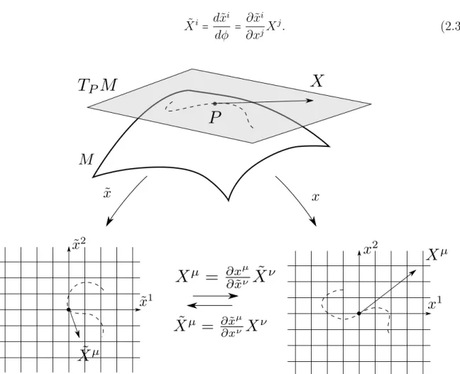
In other words, an observe who is only influenced by the gravitational field is an inertial observer – but her inertial system might not encompass all of space-time, but only a small neighbourhood around her world line. But in that coordinate system, the laws of special relativity should hold! Assume such an inertial observer has an inertial system with coordinatesξµ. Any other observer, which moves only under the influence of the gravitational field, has a world line ξµ(s)satisfying
d2ξµ
ds2 = 0. (1.68)
A general, non-inertial observer O (such as the Rindler observer) will have a different coordinate system, and might not perceive the inertially moving particles as moving along a straight line. What is the equation of motion in their coordinatesxµ?
We assume that locally the two coordinate system can be transformed into one an- other, and that xµ(ξ) and ξµ(x) are smooth and inverse to one another. This means that all partial derivatives ∂ξ∂xµν exist, are smooth, and satisfy
∂ξµ
∂xν
∂xν
∂ξρ = δµρ, ∂xµ
∂ξν
∂ξν
∂xρ = δµρ. (1.69)
We express the world line s↦ξµ(s) inO’s coordinates xµ. ONe has 0 = d2ξµ
ds2 = d ds( d
dsξµ(x(s))) = d ds(∂ξµ
∂xν dxν
ds )
= d
ds(∂ξµ
∂xν)dxν
ds + ∂ξµ
∂xν d2xν
ds2 = ∂2ξµ
∂xρ∂xν dxρ
ds dxν
ds + ∂ξµ
∂xν d2xν
ds2 . This can be expressed as:
0 = ∂xσ
∂ξµ
∂ξµ
∂xν d2xν
ds2 + ∂xσ
∂ξµ
∂2ξµ
∂xρ∂xν dxρ
ds dxν
ds . (1.70)
Using the fact that the matrices with entries ∂x∂ξσµ and ∂ξ∂xµν are inverse to one another, i.e. (1.69), we get:
d2xµ
ds2 + ∂xµ
∂ξσ
∂2ξσ
∂xρ∂xν dxρ
ds dxν
ds = 0. (1.71)
This equation of motion still contains terms which depend on the inertial coordinates ξµ, to which our observerO might not have any access (or might not be interested in).
But there is a better way to express this equation of motion, by introducing the so-called space-time metric. This is a local version of the Minkowski distance.
Consider two events close to one another, which, in the inertial observer’s system, have coordinates ξµ and ξµ+∆ξµ. Since for the inertial observer the laws of special relativity should hold, the space-time distance between the two events are
∆s2 = ηµν∆ξµ∆ξν. We express these inO’s coodrdinates xµ, and get
∆ξµ = ∂ξµ
∂xρ∆xρ + . . . , (1.72) up to terms of higher order in the ∆xρ. The partial derivatives are to be taken at xµ the coordinates of the first event. This gives us
∆s2 = ηµν∂ξµ
∂xρ
∂ξν
∂xσ∆xρ∆xσ. (1.73)
In the limit of the two events approaching one another, one gets
ds2 =∶ gρσdxρdxσ. (1.74)
where we have defined thespace-time metric gµν ∶= ηρσ∂ξρ
∂xµ
∂ξσ
∂xν. (1.75)
These are coefficients which measure the infinitesimal space-time distance between events.
Figure 1.17: Two events which are close to one another have the space-time distance
∆s2, which can be expressed with the help of the metric coefficientsgµν. If the coordinates xµ are actually inertial coordinates, we have gµν =ηµν. In general, however, gµν will be different fromηµν, and can even change from point to point.
The equation of motion (1.71) can now be expressed in terms of the metric coefficients, and their partial derivatives. This is great, because we do not need to make a reference
to an inertial observer, but can work entirely with physical quantities which can be measured entirely by O. For this we need the inverse metric gµν, which is defined by the inverse matrix to gµν, i.e.
gµνgνρ = δµρ, gµνgνρ = δρµ. (1.76) With these we define the so-calledChristoffel symbols Γµνρ, by
Γµνρ ∶= 1
2gµσ(∂gσν
∂xρ + ∂gσρ
∂xν − ∂gνρ
∂xσ). (1.77)
The Christoffel symbols are symmetric in the lower two indices.
Γµνρ = Γµρν f¨ur alle µ, ν, ρ=0, . . . ,3. (1.78) Nex we express the inerse metric in terms of the inverse Minkowski metricηµν:
gµν = ∂xµ
∂ξρ
∂xν
∂ξσηρσ. (1.79)
Insert now (1.75) into the expression of the brackets in (1.77), and we get:
∂gσν
∂xρ + ∂gρσ
∂xν −∂gρν
∂xσ (1.80)
= ηλτ( ∂
∂xρ(∂ξλ
∂xσ
∂ξτ
∂xν) + ∂
∂xν (∂ξλ
∂xρ
∂ξτ
∂xσ) − ∂
∂xσ (∂ξλ
∂xρ
∂ξτ
∂xν))
= ηλτ( ∂2ξλ
∂xρ∂xσ
∂ξτ
∂xν +∂ξλ
∂xσ
∂2ξτ
∂xν∂xρ+ ∂2ξλ
∂xν∂xρ
∂ξτ
∂xσ +∂ξλ
∂xρ
∂2ξτ
∂xν∂xσ
− ∂2ξλ
∂xσ∂xρ
∂ξτ
∂xν −∂ξλ
∂xρ
∂2ξτ
∂xσ∂xν)
= 2ηλτ ∂2ξτ
∂xν∂xρ
∂ξλ
∂xσ. (1.81)
Here we have used the symmetry of the metric: gµν =gνµ. Now we use (1.79), and get for the Christoffel symbol:
Γµνρ = ∂xµ
∂ξα
∂xσ
∂ξβηαβηλτ
∂2ξτ
∂xν∂xρ
∂ξλ
∂xσ
= ∂xµ
∂ξτ
∂2ξτ
∂xν∂xρ.
But this is exaclty the expression in (1.71), which is why we can write : d2xµ
ds2 + Γµνρdxν ds
dxρ
ds = 0. (1.82)
So in order to incorporate the gravitational force, Einstein assumed the following:
Space-time is still four-dimensional, and events can be expressed in coordinates, but the space might not have the structure of an affine space anymore.
Observers which are only being influenced by the gravitational force are the inertial observers. In their respective inertial coordinate systems ξµ. the laws of special relativity hold. But these coordinate systems do not necessarily cover all of space- time any more.
The geometry of space-time is encoded in the space-time metric gµν, which mea- sures the space-time distance between nearby events. In an inertial coordinate system gµν =ηµν, but in general (non-inertial) coordinates xµ, the metric will be different, and depend on the point. It will be a field.
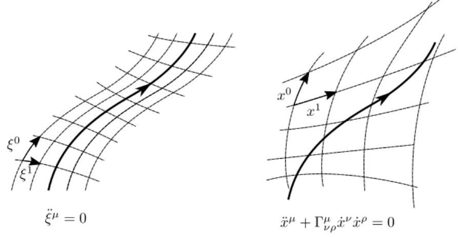
In general coordinates, the equations of motion for a particle under the influence of gravity is (1.82).
Figure 1.18: The same world line satisfies ¨ξµ =0 in the inertial coordinate system, and (1.82) in an arbitrary CS.