Tido Semmler1 , Sergey Danilov1,2,3 , Paul Gierz1 , Helge F. Goessling1 , Jan Hegewald1, Claudia Hinrichs1 , Nikolay Koldunov1 , Narges Khosravi1 , Longjiang Mu1 ,
Thomas Rackow1 , Dmitry V. Sein1,4 , Dmitry Sidorenko1 , Qiang Wang1 , and Thomas Jung1,5
1Alfred Wegener Institute, Helmholtz Centre for Polar and Marine Research, Bremerhaven, Germany,2Mathematics and Logistics, Jacobs University, Bremen, Germany,3A. M. Obukhov Institute of Atmospheric Physics, Russian Academy of Sciences, Moscow, Russia,4Shirshov Institute of Oceanology, Russian Academy of Sciences, Moscow, Russia,
5Department of Physics and Electrical Engineering, University of Bremen, Bremen, Germany
Abstract
The Alfred Wegener Institute Climate Model (AWI‐CM) participates for thefirst time in the Coupled Model Intercomparison Project (CMIP), CMIP6. The sea ice‐ocean component, FESOM, runs on an unstructured mesh with horizontal resolutions ranging from 8 to 80 km. FESOM is coupled to the Max Planck Institute atmospheric model ECHAM 6.3 at a horizontal resolution of about 100 km. Using objective performance indices, it is shown that AWI‐CM performs better than the average of CMIP5 models.AWI‐CM shows an equilibrium climate sensitivity of 3.2°C, which is similar to the CMIP5 average, and a transient climate response of 2.1°C which is slightly higher than the CMIP5 average. The negative trend of Arctic sea‐ice extent in September over the past 30 years is 20–30% weaker in our simulations compared to observations. With the strongest emission scenario, the AMOC decreases by 25% until the end of the century which is less than the CMIP5 average of 40%. Patterns and even magnitude of simulated temperature and precipitation changes at the end of this century compared to present‐day climate under the strong emission scenario SSP585 are similar to the multi‐model CMIP5 mean. The simulations show a 11°C warming north of the Barents Sea and around 2°C to 3°C over most parts of the ocean as well as a wetting of the Arctic, subpolar, tropical, and Southern Ocean. Furthermore, in the northern middle latitudes in boreal summer and autumn as well as in the southern middle latitudes, a more zonal atmosphericflow is projected throughout the year.
Plain Language Summary
The Alfred Wegener Institute Helmholtz Centre for Polar and Marine Research (AWI) participates for thefirst time with a global climate model in the Coupled ModelIntercomparison Project 6 (CMIP6). The results of CMIP6 and previous model comparison projects feed into the next assessment report of the Intergovernmental Panel on Climate Change (IPCC). The IPCC
assessment reports include information on past and expected climate change in the future and is written for policy‐and decision‐makers as well as for the general public. The main characteristics of the AWI climate model are described and compared to models from previous intercomparison projects. The projected global warming in AWI‐CM is similar to the average warming predicted by climate models in the
previous intercomparison project. However, the Arctic sea‐ice extent declines faster than typical previous estimates. Areas that are wet in present‐day climate become wetter, and areas that are dry in present‐day climate become drier in the future—consistent with previous climate model simulations. The ocean currents remain rather stable in the AWI climate projections, which leads to a continued warm Gulf stream and therefore an only slightly reduced warming of the North Atlantic and parts of Europe compared to other middle‐latitude regions.
1. Introduction
Around 50 institutions worldwide are participating in the current sixth phase of the Coupled Model Intercomparison Project 6 (CMIP6; Eyring et al., 2016). The Alfred Wegener Institute Helmholtz Centre for Polar and Marine Research in Germany contributes for thefirst time to CMIP with the novel Finite Element Sea Ice‐Ocean Model (FESOM) coupled to the atmosphere model ECHAM6 developed at Max Planck Institute (MPI) for Meteorology in Hamburg. The novelty of FESOM lies in the use of global
©2020. The Authors.
This is an open access article under the terms of the Creative Commons Attribution License, which permits use, distribution and reproduction in any medium, provided the original work is properly cited.
Key Points:
• The paper describes contributions of AWI‐CM, which employs a sea‐ice ocean component formulated on unstructured meshes, to CMIP6
• Equilibrium climate sensitivity is similar to average of CMIP5 projections; transient climate response is slightly above average
• Response patterns are similar to CMIP5 with more pronounced Arctic sea ice loss and a more stable AMOC compared to other systems
Correspondence to:
T. Semmler, tido.semmler@awi.de
Citation:
Semmler, T., Danilov, S., Gierz, P., Goessling, H. F., Hegewald, J., Hinrichs, C., et al. (2020). Simulations for CMIP6 with the AWI climate model AWI‐CM‐1‐1.Journal of Advances in Modeling Earth Systems,12, e2019MS002009. https://doi.org/
10.1029/2019MS002009 Received 21 DEC 2019 Accepted 4 AUG 2020
Accepted article online 24 AUG 2020 Correction added on 25 SEPT 2020, afterfirst online publication: Projekt Deal funding statement has been added.
unstructured meshes that only few institutions worldwide are employing at this stage (e.g., Korn, 2017;
Petersen et al., 2019). The unstructured‐mesh approach allows putting a particular focus on dynamically active regions such as the North Atlantic Current, the Southern Ocean, and the tropics while using relatively coarse resolution elsewhere. For the set of “Evaluation and Characterization of Klima” (DECK) and ScenarioMIP experiments, a mesh with local refinement of up to 8 km in the North Atlantic Current and the Southern Ocean is used. Coupling the unstructured ocean model FESOM to ECHAM6, which is also used for the MPI‐ESM contribution to CMIP6, offers the unique opportunity to investigate the influence of an alternative ocean model formulation on the results which will be exploited in further research.
Many models that participated in CMIP3 and CMIP5 have common descent and share ideas and code with each other (Knutti et al., 2013; Masson & Knutti, 2011). This leads to a clustering of results based on model
“genealogy”and challenges the assumption of model independence. The ocean part of the AWI‐CM is a new unstructured mesh model. It is thus based on a different dynamical core compared to most of the models contributing to CMIP6. Although many parameterizations in FESOM are similar to conventional structured‐grid ocean models, and although the ECHAM model has already participated since CMIP3 in the CMIP efforts (Stevens et al., 2013), it can be argued that the use of an unstructured‐mesh sea ice‐ocean model is an important contribution to the diversity of the CMIP6 ensemble. Large‐scale character- istics dominated by the formulation of the atmosphere, such as the equilibrium climate sensitivity, are not expected to be influenced too much by the ocean formulation. In contrast, the ocean has the potential to modulate the transient evolution and regional patterns of the response considerably. This can lead to differ- ences in projected changes of coupled phenomena such as the El Niño‐Southern Oscillation (ENSO) as well as sea ice in polar regions.
The aim of this paper is to present the main characteristics of the AWI‐CM in the context of the CMIP6 pro- ject based on an evaluation of selected atmosphere, ocean, and sea ice parameters for present‐day climate as well as for future climate. The evaluation of the unstructured mesh ocean component compared to the tradi- tional mesh ocean component of Max Planck Institute for Meteorology (MPIM) is beyond the scope of this study and will be the topic of a collaborative publication with the MPIM.
In section 2, a brief model description is given along with a summary of the performed DECK and ScenarioMIP simulations, following the CMIP protocol. In section 3, remaining model drift and imbalances are analyzed. Section 4 describes biases in our present‐day simulations for some important atmosphere, sea‐
ice, and ocean variables. The climate change signal is analyzed in detail in section 5. Finally, a discussion of the results and conclusions are presented in sections 6 and 7.
2. Model and Simulation Description
2.1. Model Description
The sea ice‐ocean component of AWI‐CM is the Finite Element Sea Ice‐Ocean Model (FESOM; see Danilov et al., (2004), for the sea ice component and Wang, Danilov, et al., (2014), for the ocean component). It uses unstructured meshes, that allow simulations of ocean and sea ice dynamics with variable grid resolution.
This also enables refinement in resolution for areas where small‐scale dynamics are prevalent (e.g., narrow straits and strongly eddying regions; Sein et al., 2016, 2017). Tools have been developed to enable users of FESOM data to perform analysis efficiently (see Appendix A1). Furthermore, selected variables are also available on regular latitude‐longitude meshes.
The atmospheric component of AWI‐CM is the spectral atmospheric model ECHAM6.3.04p1 from MPIM (Stevens et al., 2013) which is used here without any additional modifications or tuning. This version of ECHAM is also used in the MPIM contribution to CMIP6. Having these two setups thus will allow future intercomparisons of the coupled systems that share the same atmosphere model but use different sea ice‐ocean models.
A more detailed description of the AWI‐CM components and an evaluation of its mean state and climate variability are provided in Sidorenko et al. (2015) and Rackow et al. (2018), respectively. AWI‐CM realisti- cally simulates many aspects of the modern climate, showing an overall performance that is generally better than the most realistic climate models participating in CMIP5.
10.1029/2019MS002009
Journal of Advances in Modeling Earth Systems
The CMIP6 version of the code encompasses several changes compared to that described in Sidorenko et al. (2015) and Rackow et al. (2018). The major technical improvement involves the removal of the regular exchange mesh, which in earlier versions was used as an interface between FESOM and the OASIS3‐MCT coupler. In the CMIP6 version, the interpolation between unstructured FESOM and structured ECHAM meshes is done by the coupler. Furthermore, the coupling between ocean and atmosphere has been sped up remarkably through the use of the parallel support built in OASIS3‐MCT.
Updates of physical parameterizations in the ocean sea ice component comprise the inclusion of (1) a salt plume parameterization (Sidorenko et al., 2018) which improves the simulated sea surface salinity in the Arctic Ocean, (2) modified background diffusivities, as suggested by Wang, Danilov, et al. (2014), and (3) a K‐Profile Parameterization (KPP) for vertical mixing (Large et al., 1994) in the ocean model which has solved shortcomings related to the North Atlantic circulation, pointed out in Rackow et al. (2018) and Sidorenko et al. (2015). Those previous publications were based on simulations on different meshes and with constant rather than transient forcing. This and the fact that these simulations were performed within the CMIP6 framework according to a common protocol calls for documentation of the CMIP6 version of the model and its results presented in this paper.
2.2. CMIP6 Simulations
In this paper, the focus is on the DECK and ScenarioMIP simulations, which were defined in the CMIP6 overview paper (Eyring et al., 2016) and are summarized in Table 1. Before starting the 500‐year coupled piControl‐spinup simulation with constant pre‐industrial forcing, a 10‐year long ocean‐only simulation initialized from the EN4 ocean reanalysis (Good et al., 2013) averaged over 1950–1954 has been performed.
In these 10 years of ocean‐only simulation, the initial adjustment of the ocean state takes place. This pre‐spinup helps to ensure a numerically stable adjustment phase of the coupled system. The piControl simulation is a continuation of the piControl‐spinup simulation. From the piControl simulation, the idea- lized greenhouse gas forcing simulations 1pctCO2and abrupt‐4xCO2simulations as well as the historical for- cing simulations are branched off at specific years (branch‐off point(s); see Table 1). At the end of the historical forcing simulations, that is at the end of the Year 2014, the scenario simulations are continued with forcing prescribed from the anthropogenic forcing scenarios. These scenarios are derived from Shared Socioeconomic Pathways (SSP) (Meinshausen et al., 2019).
The idealized and historical forcing simulations have been branched off sufficiently long before the end of the piControl simulation to ensure that every year of the sensitivity simulations (idealized, historical, and scenario simulations) has a corresponding year in the piControl simulation. The climate change signal is always computed following the delta approach (e.g., Lenderink et al., 2007), that is, as the difference between the sensitivity simulation and the corresponding year(s) of the piControl simulation, to account for possible model drift.
The ECHAM model is run at a spectral resolution of T127L95, where T127 denotes a spectral truncation at total wavenumber 127, which corresponds to about 100 km horizontal resolution in the tropics and higher horizontal (zonal) resolution toward the poles—for example, about 25 km in 75° latitude. L95 stands for 95 Table 1
DECK and ScenarioMIP Simulations Performed With AWI‐CM
Experiment Experiment group Parent experiment Years Branch‐off point(s) Ensemble members
Ocean‐only spinup None None 10 years None 1
piControl‐spinup DECK Ocean‐only spinup 500 years After 10 years 1
piControl DECK piControl‐spinup 500 years After 500 years 1
1pctCO2 DECK piControl 150 years After 250 years 1
abrupt‐4xCO2 DECK piControl 150 years After 250 years 1
historical DECK piControl 1850–2014 After 150, 175, 200, 225, 250 years 5
ssp126 ScenarioMIP historical 2015–2100 End of 2014 1
ssp245 ScenarioMIP historical 2015–2100 End of 2014 1
ssp370 ScenarioMIP historical 2015–2100 End of 2014 5
ssp585 ScenarioMIP historical 2015–2100 End of 2014 1
Note. The forcing of the ScenarioMIP simulations is described in more detail in Meinshausen et al. (2019).
unevenly spaced model levels with high vertical resolution close to the surface (60 to 300 m in the atmospheric boundary layer) and reaching up to 0.01 hPa corresponding to 80 km (i.e., high‐top model version).
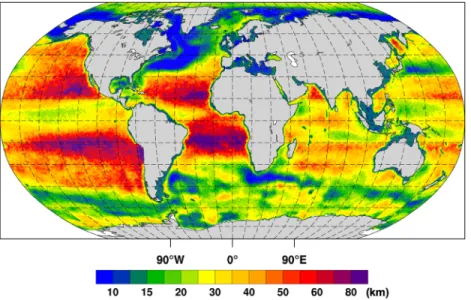
In our AWI‐CM‐1‐1‐MR CMIP6 contribution (Semmler et al., 2018), the FESOM model is run on a medium‐resolution“MR”mesh that follows the mesh design strategy proposed by Sein et al. (2016, 2017) (Figure 1): The main approach is to locally increase the resolution over areas of high sea surface height (SSH) variability as obtained from satellite data. The horizontal resolution of the mesh varies from 8 km over energetically active areas such as the North Atlantic Current region to 80 km over areas with low SSH varia- bility. The number of surface grid points of the MR mesh is close to the number of grid points in conven- tional regular model grids of ¼° resolution. The performance of the “MR‐type” meshes in a climate configuration with AWI‐CM in comparison to several other FESOM meshes is evaluated in Rackow et al. (2019), Sein et al. (2018), de la Vara et al. (2020).
2.3. Cmorization and Data Publication
CMIP6 is a community project, and sharing our experiment result data is an important aspect of the project.
To be able to utilize data from other groups, a large set of output data has been defined where the attributes and detailed description for each dataset are put in place as a reference. These are called the CMIP6 CMOR data request (DR) tables (cmip6‐cmor‐tables 2019). The tables have evolved to a great extent over the past 3 years. All CMIP6 data are being published through the Earth System Grid Federation (ESGF) (Juckes et al., 2020)—including the AWI‐CM CMIP6 data (Semmler et al., 2018).
From a technical point of view, wefirst chose which variables to generate during our model runs, as re‐running the simulations is usually not feasible due to time and resource constraints. We currently pro- duce around 150 variables matching the recent CMIP6 CMOR DR tables. The model has been optimized to be able to output the data in a very resource efficient manner; this enables us to use less computing resources and complete the simulations more quickly. Due to the many changes of the requirements regard- ing the output contents and metadata information, the CMIP6 CMOR DR tables have undergone, we had to develop aflexible strategy to transform the simulation output into the required publishable format.
As a result, we now have a post processing software in place, which can directly be fed with the aforemen- tioned DR tables to produce the output accordingly (Hegewald, 2019). More details on the procedure and an explanation of how to use unstructured mesh data from the ESGF can be found in Appendix A1.
Figure 1.Spatial resolution (in km) of the FESOM MR grid used in AWI‐CM‐1‐1‐MR for the CMIP6 DECK and ScenarioMIP simulations. Resolution is locally increased up to 8 km in regions of high sea surface height (SSH) variability as observed by satellites.
10.1029/2019MS002009
Journal of Advances in Modeling Earth Systems
3. Remaining Drift and Imbalances in the Pre‐Industrial Control Simulation
In the pre‐industrial control simulation, AWI‐CM is in quasi‐equilibrium:
The 2 m temperature drift from Year 150 to Year 400 of the piControl simulation (the time period to which most of the historical, scenario, and idealized CO2increase experiments need to be compared) amounts to 0.00022°C/year. Furthermore, sea ice trends are ranging from
−6.9 × 10²to−2.7 × 10²km2/year for the Arctic and from−4.4 × 10²to
−2.6 × 10² km2/year for the Antarctic computed for the Years 150 to 400 during March and September, respectively. This suggests that any residual drift of 2 m temperature and sea‐ice extent in the coupled system is much smaller than the changes anticipated in a warming word.
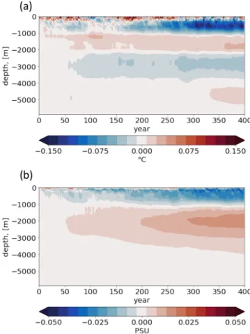
Figure 2 shows the Hovmöller diagrams for the global average profiles of oceanic potential temperature and salinity for the last 400 years of the control simulation. The amplitude of the drift is less than 0.15°C for tem- perature and 0.05 psu for salinity, respectively, indicating that the system is close to its quasi‐equilibrium state. The drift in temperature is concen- trated at depths of 500, 1,500, 3,000, and 4,500 m, while the drift in salinity happens mainly at depths of 500 and 2,000 m. From inspecting the spatial distribution of the drift (not shown), we conclude that the upper drift zone at 500 m stems primarily from the overall cooling and freshening of the ocean. The drift between 1,500 and 2,000 m is partly linked to the Mediterranean outflow which spreads into the southern North Atlantic.
The simulated outflow is too warm and too salty. At 3,000 m, we observe that the Atlantic and Pacific Oceans become cooler while Indian and Southern Oceans show positive trends in temperature. Simultaneously, salinity in the North Atlantic shows a negative trend at this depth, partly compensating the warming signal there in terms of density. Everywhere else at this depth there is a positive drift in salinity, most pronounced in the Indian Ocean. Finally, the deepest zone of temperature increase at
~4,500 m stems from a warming trend in the Southern Ocean. Although the spatial pattern of non‐zero temperature changes implies a small remaining redistribution of heat and salinity, we overall conclude that the system is close to a quasi‐equilibrium state. Simulated changes in response to greenhouse gas increases are clearly stronger than this residual drift as shown in section 5.3.
In the last 100 years of the 500‐year piControl simulation, which followed the 500‐year spinup simulation, there are still imbalances in the top‐of‐atmosphere (TOA) and net surface radiation. Averaged over these 100 years, the TOA radiation imbalance amounts to 0.34 W/m2, whereas the net surface energyflux consist- ing of radiation and turbulent heatfluxes amounts to 0.84 W/m2. Given that changes in the atmospheric energy content on this time scale are much smaller, the discrepancy implies an unphysical atmospheric energy non‐conservation of about 0.5 W/m2. By using the delta approach in the evaluation of the climate change signal as briefly introduced in section 2.2, this non‐conservation is canceled out although one needs to keep in mind the non‐linearity of the system.
The gradual energy loss of the ocean over the same time period, diagnosed from changes in the 3D ocean temperature (and sea‐ice mass changes), corresponds to a global surface energyflux of−0.01 W/m2. The deviation from the atmospheric surfaceflux imbalance by 0.85 W/m2cannot be explained by changes in the continental heat content but points to further deviations from energy conservation that can be related to mismatching grids and coastlines between the model components, inconsistent treatment of temperature, precipitation, and runoff (Mauritsen et al., 2012), or other inconsistencies. The atmosphere‐related and the surface‐related non‐conserving energy terms partly compensate each other, resulting in an overall unphysi- cal energy sink of−0.35 W/m2, and both of them are relatively constant over all simulations (when averaged over decades and longer; not shown).
Figure 2.Vertical profiles of globally averaged (a) ocean temperature and (b) salinity in the last 400 years of the 500 years of piControl simulation (relative to the beginning of this 400 year time period). The last 400 years cover all simulations branched off since thefirst branch‐off point is in Year 150 of the piControl simulation, that is, 350 years before the end of the piControl simulation (see Table 1).
4. Present‐Day Climate From Historical Simulations
4.1. Performance Indices
In order to objectively characterize the performance of the historical simulations compared to observations, we use modified performance indices by Reichler and Kim (2008) as described in Sidorenko et al. (2015) for the atmosphere and in Rackow et al. (2019) for the ocean. The referenced reanalysis and observation data the model is compared to and a description of the computation of the index are given in Appendix A2.
The index measures model error compared to observations relative to the average model error of CMIP5 models. A performance index of 0.5 would indicate an excellent performance as the mean absolute error is halved compared to the CMIP5 models while a performance index of 2 would indicate a doubling of the mean absolute error compared to the CMIP5 models.
Table 2 shows the atmosphere performance indices of thefirst ensemble member of the historical simula- tions. For the other four ensemble members of the historical simulations, the results are very similar (not shown). While the performance indices arefirst computed for each season individually, here, for brevity, we show the annual average. Globally, AWI‐CM shows a good performance in all considered variables and is better than the CMIP5 multi‐model mean. Especially Antarctic large‐scale circulation and sea ice con- centration are very well represented compared to the average of the CMIP5 models. However, there are a few variables such as precipitation, 500 hPa geopotential, and Arctic sea ice which are not in all regions repre- sented better than by the CMIP5 models (only global mean, Arctic, and Antarctic shown for brevity). As pointed out in section 5.2.2, the Arctic sea‐ice extent is very well represented both in terms of the mean value and in terms of the trend over the past 3 decades. The sea ice concentration is underestimated in boreal sum- mer and autumn in the interior Arctic—see section 4.5—but the sea‐ice extent is not affected by this since values are generally between 50% and 90% and therefore are still well above the threshold of 15%.
From the performance indices for the ocean (Table 3), we can conclude that potential temperature is better represented than in CMIP5. However, this is not the case for salinity. Salinity in the Pacific Ocean as well as in the North Atlantic Ocean deviates more from observations compared to the average of CMIP5 models.
While the performance indices give a quick and objective overview of how a model performs compared to other CMIP5 models, it is necessary to carry out more detailed analysis to investigate if typical errors of climate models such as the Southern Ocean warm bias or the cold bias in the North Atlantic subpolar gyre persist. Regarding the errors in potential temperature and salinity, more analysis is provided in section 4.4.
4.2. Atmospheric Circulation
AWI‐CM shows a too strong westerly flow above the Southern Ocean especially in austral summer, indicated by too low mean sea level pressure (MSLP) over the southern high latitudes and too high MSLP over the southern middle latitudes (Figure 3). In the Euro‐Atlantic sector, there is evidence for a southward shift of the jet stream, resulting in a too strong westerlyflow over Southern Europe and a too weak westerlyflow over Northern Europe in boreal winter and spring. This bias has been found Table 2
Atmosphere and Sea Ice Performance Indices for Years 1985–2014 of the First Ensemble Member of AWI‐CM Historical Simulations Averaged Over the Four Seasons
2‐m temperature
10‐m u‐component
10‐m v‐component
TOA outgoing longwave
radiation Precipitation Total cloud cover
500‐hPa geopotential
height
300‐hPa u‐component
Sea ice
concentration Average
Global 0.77 0.81 0.81 0.74 0.99 0.75 0.92 0.72 ‐ 0.81
Arctic 0.92 0.81 0.84 0.69 1.16 0.71 1.24 0.89 1.23 0.94
Antarctic 0.71 0.65 0.84 0.74 1.05 0.70 0.53 0.64 0.50 0.71
Note. The set of CMIP5 models consists of CCSM4, MPI‐ESM‐LR, GFDL‐CM3, HadGEM2‐ES, and MIROC‐ESM.
Table 3
Ocean Performance Indices for Years 1985–2014 of the First Ensemble Member of AWI‐CM Historical Simulations Averaged Over the Two Seasons DJF and JJA
Potential temperature Salinity Average
Global ocean 0.79 1.15 0.97
Southern Ocean 0.96 0.70 0.83
Indian Ocean 0.69 0.94 0.82
North Pacific Ocean 0.92 1.28 1.10
South Pacific Ocean 0.81 1.14 0.98
North Atlantic Ocean 0.70 1.70 1.20
South Atlantic Ocean 0.75 0.79 0.77
Arctic Ocean 0.72 0.90 0.81
Note. The set of CMIP5 models consists of ACCESS 1.3, BCC‐CSM 1.1, BNU‐ESM, CanESM2, CCSM4, CMCC‐CM, CMCC‐CMS, CNRM‐CM 5.2, CSIRO‐Mk 3.6.0, EC‐Earth, MPI‐ESM‐LR, GFDL‐CM3, GISS‐E2‐H, GISS‐E2‐R, HadGEM2‐ES, IPSL‐CM5B, MIROC‐ESM, MRI‐CGCM3, MRI‐ESM 1, and NorESM1‐ME.
10.1029/2019MS002009
Journal of Advances in Modeling Earth Systems
in numerous CMIP5 models (Zappa et al., 2013), and it can be associated with an underestimation of Euro‐Atlantic blocking (Jung et al., 2012). Especially in boreal winter, the Aleutian low is too weak. This fea- ture was observed in previous ECHAM6 simulations as well (Stevens et al., 2013). The MSLP biases are not negligible and amount to up to 7 hPa. In the regions they occur, these biases are comparable to the climate change signal indicating that the confidence in projections of circulation changes is low.
The MSLP bias is dependent on the season as shown in Figures 3a–3d. However, in the following, we will also consider the annual mean sea level pressure biases (Figure 3e) to make our results more comparable with previous studies of CMIP6 models such as Müller et al. (2018) for MPI‐ESM (their Figure 7d), using Figure 3.Mean sea level pressure (MSLP) bias (hPa) as an ensemble mean over thefive historical realizations for 1985–2014 compared to ERA5 climatology (Copernicus Climate Change Service [C3S], 2017; Hersbach et al., 2020) from 1985 to 2014. (a) DJF, (b) MAM, (c) JJA, (d) SON, (e) annual mean.
ECHAM6 as the atmosphere component like AWI‐CM. In the annual mean, biases are smaller than 1 hPa over large areas of the tropics, subtropics, and southern middle latitudes. This is consistent with results from Müller et al. (2018). However, differences to Müller et al. (2018) exist over the South Atlantic gyre where AWI‐CM shows stronger high pressure biases (2–3 hPa) compared to MPI‐ESM (1–2 hPa), and in the south‐east Pacific north of West Antarctica where AWI‐CM shows negative biases of 1–2 hPa and MPI‐ESM positive biases of 2–5 hPa. A thorough comparison between MPI‐ESM and AWI‐CM, which goes beyond the scope of this study, is planned in collaboration with MPIM.
Figure 4 shows zonal means of temperature and zonal wind biases averaged over the period 1985–2014. In large areas of the troposphere, temperature biases are smaller than 1°C. Exceptions are the high latitudes with larger positive biases in the north and larger negative biases in the south. Furthermore, in the middle and high latitudes there are negative temperature biases of up to around 3°C in the lower stratosphere around 200 hPa. Not surprisingly, the bias pattern looks very similar to the one from MPIM shown in Müller et al. (2018, their Figure 9e). The zonal mean zonal wind is generally well represented compared to the ERA5 reanalysis data. Biases are mostly smaller than 2 m/s.
Exceptions are the tropical stratosphere, the tropical upper troposphere, and the subtropical/middle‐latitude stratosphere around 100 hPa and 40–50°N and S. Compared to Müller et al. (2018, their Figure 9d), biases are generally similar although the subtropical/middle‐latitude strato- sphere areas of strong biases of more than 2 m/s are smaller in AWI‐
CM. Furthermore, the negative bias around 60°S extending from 700 to 200 hPa in Müller et al. (2018) does not exist in AWI‐CM.
4.3. ENSO Statistics and Phase Locking
Sea surface temperature (SST) anomalies in the tropical Pacific associated with the El Niño‐Southern Oscillation (ENSO) are of global concern.
Since ENSO is the largest signal of interannual variability on Earth (e.g., Timmermann et al., 2018), the realistic simulation of these SST anomalies, both with respect to their absolute magnitude and temporal behavior, is crucial for any global climate model.
When comparing area‐weighted SST anomalies in the Niño 3.4 box (170°W to 120°W, 5°S to 5°N) to observations, wefind that thefive histor- ical ensemble members with AWI‐CM show a realistic distribution (Figure 5). The clear asymmetry between El Niño and La Niña events Figure 4.(a) Annual mean zonal mean temperature (°C) and (b) annual mean zonal mean zonal wind (m/s) as an ensemble mean over thefive historical realizations for 1985–2014 compared to ERA5 climatology (Copernicus Climate Change Service [C3S], 2017; Hersbach et al., 2020) from 1985 to 2014. Solid lines represent temperatures at or above 0°C and westerly zonal wind speeds from the ERA5 climatology, dashed lines represent temperatures below 0°C and easterly wind speeds, and contours represent biases.
Figure 5.Probability distribution function (PDF) of sea surface temperature anomalies in the Niño 3.4 region for the historical period 1870–2014. The black line gives the observed Niño 3.4 PDF for the period 1870–2014 (Rayner et al., 2003), available for download from the National Oceanic and Atmospheric Administration (NOAA, https://www.esrl.noaa.
gov/psd/gcos_wgsp/Timeseries/Nino34/).The ensemble‐mean of thefive historical members is given in blue; their range (min/max) is shaded in light blue.
10.1029/2019MS002009
Journal of Advances in Modeling Earth Systems
seen in observations (positive skewness of Niño 3.4 SST anomalies) is also evident in the model. The skewness is 0.15 ± 0.16 (one standard deviation) in thefive ensemble members while the observed skewness is 0.36 for 1870–2014. Note that all data have been linearly detrended and the seaso- nal cycle has been removed before computing the standard deviation.
Moreover, the Niño 3.4 index has a significant broad spectral peak, both in the model and in observations for 1870–2014, at a typical period of about 4–7 years when compared to corresponding red‐noise processes (Figure 6). While the distribution of the variance over the frequencies is well reproduced in the model, the total variance is overestimated in all AWI‐CM‐MR ensemble members (0.75–1.01 K2compared to the observed 0.57 K2).
To assess the temporal behavior further, we apply a diagnostic that quan- tifies the seasonal phase locking of Niño 3.4 SST anomalies to the seasonal cycle (Figure 7). Observed SST variability associated with ENSO, as diag- nosed from monthly standard deviation, tends to peak in boreal winter, with a minimum in spring. Especially in boreal winter, thefive ensemble members capture the corresponding U‐shape and its magnitude relatively well; however, there is a positive bias in spring. A bias of similar magni- tude had already been identified in a previous configuration of AWI‐ CM, using a globally relatively low resolution mesh but with tropical ocean grid refinement at 0.25° (Rackow & Juricke, 2020). The bias appears to be rather sensitive to the applied tropical ocean resolution since the sec- ondary peak in spring is much stronger at a coarser resolution of 1°, using the same atmospheric resolution (see Figure 6 in Rackow et al., 2014).
4.4. Ocean
Spatial distributions of temperature and salinity biases at the surface and in the interior of the ocean for historical simulations are shown in Figure 8. Most areas show a small cold bias of 1°C or less in sea surface temperature (SST). There is a pro- nounced cold bias in the North Atlantic, which is related to the too zonal pathway of the North Atlantic Current; this is a problem that is present in many CMIP climate models (e.g., Wang, Zhang, et al., 2014).
Figure 6.Power spectral densities (PSDs) of sea surface temperature anomalies in the Niño 3.4 region for the period 1870–2014. The black line gives the observed (OBS) spectrum after Rayner et al. (2003). Thefive historical ensemble members with AWI‐CM are given in blue. Gray shading denotes the 5–95% confidence interval of an AR(1)‐processfitted to OBS, based on a Monte Carlo approach with 10,000 realizations, as detailed by Rackow et al. (2018). The total (integrated) observed Niño 3.4 variance [K2] is 0.57; for AWI‐CM‐MR, the range is (0.75–1.01).
Figure 7.Seasonal phase locking of sea surface temperature anomalies in the Niño 3.4 region for 1870–2014. Black dots give the monthly standard deviation of the observed Niño 3.4 index for 1870–2014 (Rayner et al., 2003); blue lines give the standard deviations of the simulated Niño 3.4 indices for each of thefive historical ensemble members (hist1 to hist5). The range (min/max) spanned by the model results is shaded in light blue. All data have been linearly detrended and the seasonal cycle removed before computing the standard deviation.
If refining the horizontal resolution further to half of the local Rossby radius which for the long time periods of CMIP6 simulations is computationally prohibitive, this bias is largely reduced (Sein et al., 2017). Warm SST biases of up to 1.5°C can be found over the Kuroshio extension, west of Africa as well as very localized close to the equator west of South America, in the Irminger current, over the Labrador Sea, and in the Southern middle latitudes in the Indian and Atlantic sector. Some of these biases are typical for climate mod- els such as the cold bias over the North Atlantic subpolar gyre or the warm bias west of Africa. However, over the Southern Ocean, no pronounced warm bias is found. This is in stark contrast to MPI‐ESM‐1.2, the cli- mate model with the same atmospheric component but different ocean model (Müller et al., 2018, their Figure 2b), and the E3SM model (Golaz et al., 2019, their Figure 10c), while there are other CMIP models that represent Southern Ocean temperature well.
At the surface, most of the ocean exhibits a fresh bias. In many subtropical and tropical areas, this bias amounts to 0.5 to 1 psu; it tends to be weaker in middle‐latitude areas. Pronounced but localized salt biases of around 2 psu can be seen close to the coasts of the Eurasian Arctic, in and around the Gulf of Mexico, and in the Bay of Bengal. Smaller salinity biases of up to 0.3 psu can be found over the Southern Ocean and the Pacific warm pool. The general feature of a surface fresh bias in many regions is present also in other climate models such as the E3SM (Golaz et al., 2019), although the regional distribution is not necessarily the same.
Features such as the Gulf of Mexico and Bay of Bengal salinity biases are in common with E3SM.
Many CMIP5 models that have coarse ocean resolution suffer from a warm bias at around 1,000 m, which is especially strong in the Atlantic Ocean. Increase in the horizontal resolution leads to reduction of this bias, as pointed out by Rackow et al. (2019). Therefore, the performance of AWI‐CM in Atlantic temperature is improved compared to other CMIP models. In the AWI‐CM simulations discussed in this paper, the magni- tude of the warm bias in the South Atlantic is similar to the one over most of the Pacific Ocean (Figure 8b).
The cold and fresh bias in the North Atlantic is related to the outflow and spreading of Mediterranean waters Figure 8.Bias of the annual mean potential temperature (°C) (a) at the surface, (b) at 1,000 m depth averaged over 1985–2014 of thefirst ensemble member of historical simulations compared to the Polar Science Center Hydrographic Climatology (PHC, updated from Steele et al., 2001). Panels (c) and (d) as (a) and (b) but for salinity (psu).
10.1029/2019MS002009
Journal of Advances in Modeling Earth Systems
from the Strait of Gibraltar. The reasons for this bias and possible ways to reduce it are discussed in Rackow et al. (2019). The positive temperature and salinity biases in the Indian Ocean are most probably related to excessive supply of warm and salty water from the Red Sea. Generally, the biases in temperature and salinity compensate each other in terms of density.
It turns out that below a depth of about 500 m in the ocean, the mean absolute error of the potential tempera- ture is smaller in AWI‐CM than in most of the CMIP5 models (Figure 9a), while for salinity, AWI‐CM is comparable to CMIP5 models (Figure 9c). Compared to the CMIP5 version of MPI‐ESM, which shares a slightly older version (6.0 instead of 6.3) of the same atmosphere component and which is run at T63 corre- sponding to around 200 km horizontal resolution instead of T127 corresponding to around 100 km horizon- tal resolution, the potential temperature error is smaller in AWI‐CM but the salinity error larger. When focusing on the North Atlantic Ocean, potential temperature (Figure 9b) for which various models show a pronounced warm bias in 1,000 to 2,000 m (Rackow et al., 2019), AWI‐CM performs well. However, for sali- nity, in the North Atlantic (Figure 9d) and also in the Pacific (not shown), the mean absolute error is large Figure 9.Profiles of mean absolute error calculated from each grid point for the (a) global ocean and (b) North Atlantic Ocean potential temperature (°C) for DJF 1985–2014 of thefive ensemble members of the historical AWI‐CM simulation (in colors) and for DJF 1976–2005 of CMIP5 simulations (in gray, each line representing one CMIP5 model, green representing the MPI‐ESM CMIP5 model). Panels (c) and (d) as (a) and (b) but for salinity (psu). The reference climatology is the Polar Science Center Hydrographic Climatology (PHC, updated from Steele et al., 2001).
compared to most of the CMIP5 models including MPI‐ESM. Note that Figure 9 shows results for DJF; for JJA, results are very similar below around 300 m.
4.5. Sea Ice
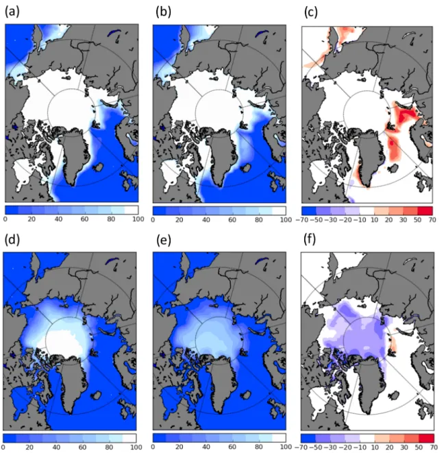
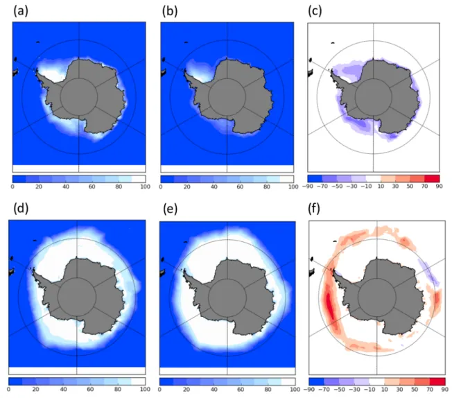
The general patterns of observed Arctic and Antarctic sea ice concentration are well represented in AWI‐CM over the last 30 years of historical simulations (Figures 10 and 11). Both Arctic and Antarctic sea ice concen- tration are overestimated in late winter in the marginal ice zones and underestimated in late summer in most areas. This hints to a too pronounced annual cycle of sea ice cover which can also be seen in the sea‐ice extent as shown in Figure 15. Nevertheless, Arctic sea‐ice extent and thickness are remarkably well represented especially over the last few years (Figures 15 and 16). While late winter Arctic sea ice concentra- tion biases are very similar to MPI‐ESM, late winter Antarctic sea ice concentration in MPI‐ESM has a sub- stantial negative bias especially northeast of the Weddell Sea and a slight negative bias in East Antarctic marginal seas (Müller et al., 2018, their Figure 4) rather than a slight positive bias. This difference is consis- tent with the reduced Southern Ocean warm bias in AWI‐CM compared to MPI‐ESM.
Figure 10.Arctic sea ice concentration (%) averaged over March 1985 to 2014 from (a) observations from the sea ice portal meereisportal.de (Grosfeld et al., 2016), (b) ensemble mean AWI‐CM historical simulations, (c) ensemble mean AWI‐CM historical simulation bias. Panels (d) to (f) same as (a) to (c) but for September 1985 to 2014.
10.1029/2019MS002009
Journal of Advances in Modeling Earth Systems
5. Climate Response
5.1. Climate Sensitivity
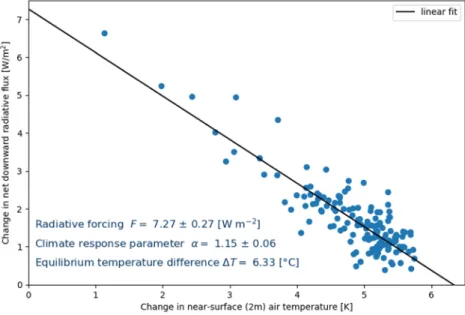
MPI‐ESM has been explicitly tuned to have an equilibrium climate sensitivity (ECS) of 3.0°C (Müller et al., 2018). The ECS is inferred from linear regression of the top‐of‐atmosphere (TOA) imbalance against the temperature response in the 4xCO2simulation. AWI‐CM uses the same atmospheric component without any extra tuning so that differences both in the ECS and in the transient climate response (TCR), computed as average response over the 30 years around Year 70 from the 1pctCO2simulation, are only due to the dif- ferent ocean component.
For AWI‐CM, the ECS amounts to 3.2°C (Figure 12, half of the 4xCO2equilibrium temperature difference).
This is similar to the average over the CMIP5 models (IPCC, 2014) and slightly larger than for the CMIP6 version of MPI‐ESM (3.0°C; Mauritsen et al., 2019; Müller et al., 2018; Tokarska et al., 2020). The TCR amounts to 2.1°C, which is slightly stronger than the average over the CMIP5 models (1.8°C; IPCC, 2014) and the CMIP6 version of MPI‐ESM (1.7°C; Tokarska et al., 2020). Note that by considering changes in the TOAflux and the global‐mean near‐surface temperature (delta approach), our estimates for the ECS and the TCR are not affected by the imbalances reported in section 3 (apart from possible non‐linear effects).
It seems that AWI‐CM absorbs energy in the deep ocean more slowly compared to MPI‐ESM. However, this hypothesis needs to be confirmed through a thorough analysis in a joint effort with the Max Planck Institute for Meteorology. Ideally, the ECS should not be affected. However, since the Gregory method to compute ECS is only an approximation, small differences can still occur.
Figure 11.(a–f) Same as Figure 10 but for Antarctica.
Changes in the energy budget and the role of shortwave feedback in the historical and scenario simulations are detailed in section 5.4.
5.2. Surface Response
5.2.1. Two Meter Temperature and Precipitation
The evolution of the global and hemispheric mean temperature at 2 m above the surface in the piControl, historical, and scenario simulations is shown in Figure 13. The piControl simulation shows no discernible trend in temperature, as expected. When considering the anthropogenic forcing, the historical simulations show a warming of 1.1 ± 0.1°C in 2005–2014 compared to 1891–1900 while for the observations the warming amounts to 0.9°C over the same period. Both in the observations and in the historical simulations, the Northern (Southern) Hemisphere warming is 0.2°C higher (lower) than the global average. The more pro- nounced warming over the Northern Hemisphere compared to the Southern Hemisphere is partly due to the higher land partition in the Northern Hemisphere compared to the Southern Hemisphere.
Until the end of the 21st century, the global mean temperature rises by approximately 4°C from today under the strongest emission scenario SSP585. Over the Northern Hemisphere, this warming is more pronounced and amounts to approximately 5°C; over the Southern Hemisphere, the warming is limited to approximately 3°C. For the weakest emission scenario, SSP126, the global mean warming remains just below 2°C compared to pre‐industrial conditions. The SSP126 scenario has been designed to keep global warming below 2°C—a condition that seems to be fulfilled in our simulations. Overall, the temperature increase in the AWI‐CM simulations for both the strongest and the weakest emission scenario agrees with the CMIP5 multi‐model ensemble mean (IPCC, 2014, their Figure SPM.6a) and appears to be slightly stronger compared to the CMIP6 version of MPI‐ESM—which is expected due to the slightly higher transient climate response in AWI‐CM compared to MPI‐ESM.
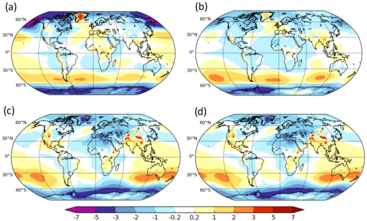
Figure 14 shows the spatial distribution of simulated temperature and precipitation changes until the end of the 21st century according to the strongest emission scenario SSP585. Temperature changes are very robust and exceed the 2 standard deviations of interannual variability of the control simulation over the whole globe (Figure 14a). Generally, precipitation changes are less robust (Figure 14b) with the Arctic and the Southern Ocean as well as the African tropics being prominent exceptions. Simulated precipitation Figure 12.Gregory plot (Gregory et al., 2004) from the abrupt‐4xCO2compared to the piControl simulation. For each year, the near‐surface (2 m) air temperature change between abrupt‐4xCO2and piControl simulation is plotted against the change in net downward radiativeflux between the two simulations. The more the abrupt‐4xCO2simulation approaches the equilibrium, the smaller the difference in net downward radiativeflux compared to the reference simulation becomes. To compute the initial radiative forcing, a regression is built from all data points and extrapolated to a change in near‐surface air temperature of 0°C.αis the climate response parameter, indicating the strength of the climate system's net feedback (radiative feedback divided by temperature response). To compute the equilibrium temperature difference, the regression is extrapolated to the equilibrium (difference in net shortwave radiation = 0).
10.1029/2019MS002009
Journal of Advances in Modeling Earth Systems
changes can be regarded as less robust than temperature changes not only because of large internal variability of the precipitation but also because of large biases in present‐day climate which amount to more than 7 mm/day in some tropical areas. Bias patterns for both 2 m temperature and precipitation as well as the magnitude of the biases for present‐day climate are not surprisingly very similar to the ones in MPI‐ESM (Müller et al., 2018, their Figure 7f).
The well‐known feature of Arctic amplification, and to a lesser extent also Antarctic amplification, can clearly be seen from Figure 14a. According to the SSP585 scenario, the temperature increases as much as 11°C over the Northern Barents Sea and around Spitsbergen. In the northernmost parts of the European and American continents, the warming exceeds 7°C at the end of the century compared to the historical reference period. Large continental areas are affected by temperature increases of more than 5°C. Also, Figure 13.Mean 2 m temperature anomaly (°C) for (a) the whole globe, (b) Northern Hemisphere, and (c) Southern Hemisphere from piControl, historical, and scenario simulations. Anomalies were computed relative to the period 1951–1980. The purple line indicates the observed 2 m temperature anomaly from Goddard Institute for Space Studies (GISS) Surface Temperature Analysis (GISTEMP v4) (GISS, 2019; Hansen et al., 2010; Lenssen et al., 2019).
over the Weddell Sea and over parts of Antarctica, temperature increases of more than 5°C are simulated. Over the ocean, the warming generally amounts to 2–3°C.
Over large areas of central Africa and over the tropical Pacific, precipita- tion increases of more than 50% are simulated. Other areas, with compar- able precipitation increases, include the ocean northwest of South Africa as well as northeastern parts of Greenland. Over the whole Arctic, a sub- stantial precipitation increase of more than 40% is simulated; over the Southern Ocean adjacent to the Antarctic continent, extended areas are affected by precipitation increases of 20% to 30%. These precipitation changes are very robust since they exceed twice the interannual standard deviation of the control simulation. Except for parts of the Amazonas region, simulated precipitation decreases are less robust and are mainly concentrated in subtropical areas. They do not exceed 50% of present‐day precipitation.
Compared to the multi‐model CMIP5 ensemble (IPCC, 2014, Summary for Policymakers, their Figure SPM.8), the temperature response in AWI‐CM looks very similar, both regarding magnitude (11°C over Northern Barents Sea, more than 5°C over large continental areas as well as Weddell Sea and parts of Antarctica, 2°C to 3°C over large parts of the ocean) and pattern of response. However, the warming hole, that is, a lack of warming over the North Atlantic subpolar gyre, that is present in the CMIP5 ensemble (e.g., Chemke et al., 2020; Menary &
Wood, 2018), hardly exists in AWI‐CM. Furthermore, the precipitation increase in AWI‐CM over the Arctic is less pronounced and the precipita- tion increase over Africa clearly more pronounced compared to the multi‐model CMIP5 ensemble (IPCC, 2014, Summary for Policymakers, their Figure SPM8). Otherwise, the precipitation response pattern is quite consistent.
It can be concluded that especially the temperature response pattern with strong Arctic and continental as well as weak ocean warming agrees very well with the multi‐model ensemble mean of CMIP5 simulations, even in terms of magnitude. Also the feature of wetting polar, subpolar, and tropical regions as well as drying subtropical regions agrees with patterns from the multi‐model ensemble of CMIP5 simulations although the magnitude of the response is not as consistent as the magnitude of the temperature response.
5.2.2. Sea‐Ice Extent
The simulated changes in sea‐ice extent are shown in Figure 15 for the Arctic (a, b) and the Antarctic (c, d) during March and September according to piControl, historical, and tier 1 scenario experiments (i.e., ssp126, ssp245, ssp370, and ssp585), along with observations of the last decades.
The strongest decline trend in sea‐ice extent can be seen in the Arctic, during September (Figure 15b).
Starting between 2025 and 2030, there are isolated years with virtually sea ice‐free Arctic summers (1 × 10⁶km2 sea‐ice extent or less) independent of climate change mitigation efforts (see also Notz &
SIMIP Community, 2020). Starting from around 2050, except for SSP126, there are subsequent summers of a virtually ice‐free Arctic ocean. The observed September sea‐ice extent according to AWI's Sea Ice Portal (Grosfeld et al., 2016; derived from the University Bremen AMSR‐ASI product; see Spreen et al., 2008) for 1979 to 2019 is shown (in purple) on top of AWI‐CM outputs, confirming that AWI‐CM sea‐ice extent agrees well with observations both in terms of the average and in terms of the rate of sea ice decline.
However, the September Arctic sea ice concentration is underestimated in AWI‐CM simulations of the last 30 years as shown in section 4.5. This needs to be taken in consideration when interpreting the projections of the future Arctic sea ice cover. According to the multi‐model CMIP5 ensembles of September sea‐ice extent, Arctic sea ice was melting even faster than predictions, even though observations remained within thefirst standard deviation of the models due to high internal variability of the participating models (Stroeve &
Notz, 2015). In comparison to CMIP5, AWI‐CM shows stronger sensitivity to the forcings. Unlike Figure 14.(a) Annual mean 2 m temperature and (b) precipitation
response according to the SSP585 scenario 2071–2100 compared to the historical period 1985–2014. Dotted (hatched) areas represent areas where simulated changes are larger than (smaller than) 2 standard deviations (1 standard deviation) of the internal variability based on yearly means of the 500‐year control simulation.
10.1029/2019MS002009
Journal of Advances in Modeling Earth Systems
multi‐model CMIP5 ensembles, ice‐free Septembers will be expected not only for SSP585 (corresponding to RCP 8.5 in CMIP5) but also for SSP245 (corresponding to RCP 4.5 in CMIP5) and SSP370 (new pathway).
IPCC AR5 reported September sea‐ice extent reduction in 2081–2100 with respect to the average of the last 20 years of historical experiments (1986–2005) to be 43% for RCP 2.6 and 94% for RCP 8.5 (IPCC, 2013, p. 92). According to our simulations, the September Arctic sea‐ice extent declines by the end of this century (2081–2100) with respect to the last 20 years of historical experiments (1995–2014) according to AWI‐CM SSP126 and SSP585 are 64% and 99.99%, respectively. The inter‐ensemble variability for both historical and scenario (ssp370) experiments is small. This means that the results are robust against internal variability.
Likewise, Arctic sea‐ice extent during March shows a continuously negative trend for historical and scenario experiments (Figure 15a). This negative trend seems to be independent of the scenario until the mid‐21st century which implies that the impact of mitigation efforts might not be seen before that in terms of Arctic winter sea ice. However, afterwards, sea‐ice extent stabilizes at around 14 × 106km2for SSP126 and SSP245. As detailed in Figure 15a, scenarios incorporating higher radiative forcings (SSP370 and Figure 15.(a) March and (b) September sea‐ice extent in the Arctic (million km2). Panels (c) and (d) same as (a) and (b) but for the Antarctic region. The purple line indicates the observed sea‐ice extent from the sea ice portal meereisportal.de (Grosfeld et al., 2016). For comparison, observational National Snow and Ice Data Center (NSIDC) (Fetterer et al., 2017) and ERA5 reanalysis (Copernicus Climate Change Service [C3S], 2017; Hersbach et al., 2020) sea‐ice extent are shown in inlays along with the ones from sea ice portal. The observation uncertainty is small and does not affect the conclusions.
SSP585) predict accelerating decline of sea‐ice extent. According to the high‐end scenario of SSP585, by 2100, Arctic March sea‐ice extent will be half of its value at the beginning of the century.
IPCC AR5 (Climate Change 2014; IPCC, 2014; Synthesis Report p. 48) reported low confidence in near‐term projections of Antarctic sea‐ice extent. This was due to the mismatch between CMIP5 models (strong simu- lated decline) and observations (no decline) along with very limited understanding of the origin of this mis- match. According to IPCC AR5, it is suspected that this phenomenon is likely due to regional variability within the Antarctic (IPCC, 2013, p. 303). A study of individual CMIP5 models also suggested that although these models cannot replicate the observed Antarctic sea‐ice extent trend, the observation still remains within the natural variability of better performing models (Turner et al., 2015). Furthermore, Bintanja et al. (2013) showed that this sea‐ice expansion could indeed be due to Antarctic sea ice shelf melting, which is not represented in CMIP5 models.
Similar to CMIP5 models, AWI‐CM predicts declining Antarctic sea‐ice extent for both September and March over recent decades (Figures 15c and 15d)—which is in contrast to observations—and furthermore till the end of the century. In addition, the simulated difference between late winter and late summer Antarctic sea‐ice extent is more pronounced than in observations. Overall, interannual variability for Antarctic sea‐ice extent is larger than for the Arctic, which agrees with thefindings regarding CMIP5 models by Turner et al. (2015). Similarly, to the Arctic sea ice, mitigation efforts only start to have a noticeable impact from around 2050.
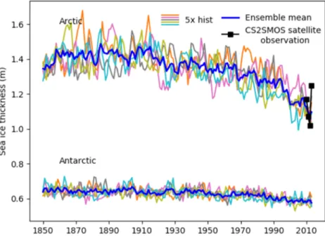
Like for the sea‐ice extent, the decline of Arctic sea‐ice thickness is also evident from the historical simula- tion during the freezing season, most pronounced from around mid‐20th century till recent years (Figure 16). Simulated sea ice thickness in the Antarctic shows a weaker decline than that in the Arctic.
We compare the simulated ensemble mean thickness in the Arctic with recent satellite thickness data from CS2SMOS (Ricker et al., 2017), which is constructed by merging CryoSat‐2 and SMOS thickness together using the optimal interpolation method. Sea ice thickness in the historical simulation falls well into the observed range from 2010 to 2013. Basin‐scale observations for sea ice thickness in the Antarctic are rather limited. A more detailed evaluation against observations for Antarctic ice thickness is therefore currently not possible.
Figure 16.Sea ice thickness in the historical simulation during the frozen season in the Arctic (averaged over December to March for each year) and the Antarctic (averaged over May to September for each year). The blue lines show the ensemble mean of thefive members indicated by different colors. Satellite estimates for the Arctic from merged CryoSat‐2 and SMOS data (CS2SMOS product) are shown by black squares.
10.1029/2019MS002009
Journal of Advances in Modeling Earth Systems
5.3. Large‐Scale Circulation Response
Similar to other climate models and as stated before, large‐scale circulation exhibits biases of the same order of magnitude as the simulated response to anthropogenic forcing affecting the reliability of the projections.
Nevertheless, a few features are worth mentioning:
The mean sea level pressure (MSLP) response to increasing greenhouse gas concentrations (Figure 17) is generally characterized by low anomalies over the polar regions and high anomalies in the southern middle latitudes. Considering the geostrophic balance, this leads to an increase of the westerlyflow in the northern and southern middle latitudes mostly around 60° latitude. Over the Northern Hemisphere, this increase is most pronounced in boreal autumn (SON) and winter (DJF). In the North Atlantic region, the increase of the westerlyflow is located further to the north compared to the CMIP5 ensemble mean as can be seen from Zappa & Shepherd, 2017, their Figure 1), while in the North Pacific region, the location of the increase of the westerlyflow is comparable. An intensified Aleutian low in boreal winter leads to a shift of the increased westerlyflow over the North Pacific sector toward lower latitudes with a maximum around 45°N. Over the Southern Hemisphere, the increased westerlyflow is equally present in all seasons with a shift in the African sector toward lower latitudes in austral winter (JJA) and spring (SON).
Figure 18 shows the zonal mean temperature and zonal mean zonal wind response to scenario forcing. The typical global warming signature with pronounced upper tropospheric tropical warming and near‐surface polar warming occurs in AWI‐CM as expected. The strongest warming in excess of 6°C occurs in the Arctic boundary layer north of 70°N—known as Arctic amplification. The upper tropospheric tropical warming amounts to 4–6°C while the Antarctic warming is limited to around 4°C. Strongest zonal mean zonal wind changes occur in the stratosphere around 100 hPa with increases in the westerly wind speed by around 5 m/s in 30–40°N and in 30–50°S. Around 60°S, there are increases in the westerly wind speed by around 1 to 2 m/s throughout the troposphere. This pattern is very similar to the multi‐model mean of CMIP5 (IPCC, 2013, chapter 12, their Figure 12.19).
Figure 17.Mean sea level pressure (MSLP) response in SSP370 scenario simulations (2071–2100) compared to historical simulations (1985–2014). For both the scenario and the historical simulations, thefive member ensemble means have been computed. (a) DJF, (b) MAM, (c) JJA, (d) SON.
There is an ongoing discussion on how the waviness of the atmosphericflow in middle latitudes will change in the future as a result of changes in the Arctic, through Arctic amplification, and in the tropics, through upper tropospheric warming. The contrasting driving from the Arctic versus the tropics has been termed a tug of war in the middle latitudes (e.g., Barnes & Polvani, 2015; Blackport & Kushner, 2017; Chen et al., 2020) Will there be a more zonalflow with a decrease in the intensity of atmospheric waves implying less extreme warm and cold events or will the meridionality of theflow get stronger implying more extreme warm and cold events in the middle latitudes or will there be no change? To answer this question, various different objective indices have been defined. Cattiaux et al. (2016) defined the sinuosity index (SI) as the length of an isohypse of a specific value divided by the length of the 50°N latitude circle. If due to features such as cut‐off lows there are separated isohypses of the specific value, the sum of the lengths of these isohypses is taken. The value of the isohypse is chosen as the area average of z500 over 30 to 70°N to accommodate for seasonal differences and climate change signals. If the SI equals to 1, theflow is zonal since the chosen iso- hypse is a straight line. The higher the SI, the stronger the meridional component of the atmosphericflow.
Figure 19 shows the SIs computed for the piControl, historical, scenario simulations, and the ERA5 reana- lysis. Overall, the differences between the different simulations are smaller than differences between the model and reanalysis data. In all simulations, the waviness of theflow is more pronounced in boreal winter and spring compared to summer and autumn. The annual cycle is shifted compared to the ERA5 reanalysis.
While the simulations show the maximum of waviness around February, according to the ERA5 reanalysis, it is around May. The minimum of waviness occurs around August in the simulations and around October according to the ERA5 reanalysis. While the amount of the maximum waviness is well captured in the model compared to the reanalysis, the minimum is too pronounced in the simulations indicating a too zonalflow in late summer.
Generally, a pronounced interannual variability can be seen both in the simulations and in ERA5. With increasing greenhouse gas concentrations, there is a tendency toward a more zonalflow in boreal summer and autumn, while in winter and spring, there is no robust change. This is consistent with the proposed tug‐ of‐war (e.g., Barnes & Polvani, 2015; Blackport & Kushner, 2017; Chen et al., 2020): the upper tropospheric warming in the tropics leads to an increased meridional temperature gradient, stronger mean westerlyflow, and decreased waviness. In contrast, in boreal winter, the effect of Arctic amplification leads to a reduced meridional temperature gradient, weaker mean westerlyflow, and increased waviness offsetting the impact of upper tropospheric warming in the tropics. However, the impact on the waviness is very much under debate and shows very little robustness. Due to the lack of Arctic amplification in boreal summer, the upper tropospheric warming in the tropics (Figure 18a) may lead to a stronger zonal and less wavyflow. However, even in boreal summer, differences are small compared to the strong interannual variability. Averaged over the year, the zonal mean zonal wind mainly increases in the stratosphere and only to some extent in the Figure 18.(a) Zonal mean temperature response (°C), (b) zonal mean zonal wind (m/s) response SSP370 scenario simulations (2071–2100, annual means) compared to historical simulations (1985–2014) (shaded contours). For both the scenario and the historical simulations, thefive member ensemble means have been computed. The solid black lines represent positive values from the historical simulations and the dashed black lines negative values.
10.1029/2019MS002009