Articles
https://doi.org/10.1038/s41559-020-1256-9
1Plankton Ecology Lab, Institute for Chemistry and Biology of the Marine Environment, Carl von Ossietzky University Oldenburg, Oldenburg, Germany.
2Helmholtz-Institute for Functional Marine Biodiversity at the University of Oldenburg (HIFMB), Oldenburg, Germany. 3Alfred-Wegener-Institute, Helmholtz Centre for Polar and Marine Research, Bremerhaven, Germany. 4School of Natural Sciences, Department of Zoology, Trinity College Dublin, Dublin, Ireland. 5Department of Physiological Diversity, Helmholtz Center for Environmental Research – UFZ, Leipzig, Germany. 6German Centre for Integrative Biodiversity Research, Leipzig, Germany. 7Martin Luther University Halle-Wittenberg, Halle, Germany. 8MARUM – Center for Marine Environmental Sciences, University of Bremen, Bremen, Germany. 9Tvärminne Zoological Station, University of Helsinki, Hanko, Finland. 10Marine Geochemistry, Institute for Chemistry and Biology of the Marine Environment, Carl von Ossietzky University Oldenburg, Oldenburg, Germany. 11Centre for Biodiversity Theory and Modelling, Theoretical and Empirical Ecology Station, CNRS and Paul Sabatier University, Moulis, France. 12Theoretical Physics/
Complex Systems, Institute for Chemistry and Biology of the Marine Environment, Carl von Ossietzky University Oldenburg, Oldenburg, Germany.
✉e-mail: helmut.hillebrand@uni-oldenburg.de
C oncepts of thresholds, tipping points and regime shifts domi- nate current ecological frameworks aiming to understand ecosystem responses to anthropogenic global change1–4. A threshold corresponds to a level of environmental pressure that creates a discontinuity in the ecosystem response to this pressure.
Thresholds and tipping points pervade environmental policy docu- ments
5,6as they allow definition of levels of pressure below which ecosystem responses remain within ‘safe ecological limits’
6and above which response magnitudes and their variances increase dis- proportionately
7,8. Anticipating when and under what conditions such threshold transgression might occur is important for sustain- able environmental management.
Threshold-related concepts and their implementation in policy hinge upon the assumption that the presence of thresholds can be detected in data or—even better—predicted. Testing this assumption requires knowledge of the ecosystem response to an environmental pressure for present-day and potential future pressure magnitudes.
Ecological meta-analysis has led to the publication of thousands of effect sizes in response to in-situ trends or experimental manipu- lations of key pressures of global change such as eutrophication, warming, land-use change, fisheries and ocean acidification. Each study in a meta-analysis quantifies the magnitude of the response of an ecosystem variable to the strength of an applied environmental pressure (Fig. 1a). The entire set of studies in the meta-analysis then represents a wide range of pressure strengths, which often exceed the conditions observed in nature but might be expected in future
ecosystems. We capitalize on this richness of data by combining available information from 36 meta-analyses, providing 4,601 effect sizes across ecosystems and pressures of global change into mul- tiple tests of whether these datasets—individually or aggregated—
reveal a response pattern that indicates transgression of a threshold (Fig.
1b). We first tested whether and how ecosystems respond toincreased environmental pressures by simply exploring whether ecosystems show a directional change in response to a pressure, regardless of the presence of a threshold (Fig. 1c). Second, we quan- tified discontinuities in the variance of responses, which would be a way to define the existence of a threshold. Finally, we tested for exis- tence of multimodality of responses, which would be stronger evi- dence for alternative states under different environmental pressures.
Results
To test for general changes of systems along gradients of envi- ronmental pressures, we used an averaged Kullback–Leibler (KL) divergence method (see Methods) to quantify the overall deviation between the response distribution for a given stressor value and the marginal response distribution; that is, the response distribu- tion when collapsing all response data onto a single axis ignoring the magnitude of the stressor variable. Most meta-analyses (23 of 36) showed changes in the response magnitude along the gradi- ent of pressure strengths (KL; Supplementary Table 1). This pro- vides strong evidence that direction and increasing magnitude of global environmental pressures have significant effects on ecosystem
Thresholds for ecological responses to global change do not emerge from empirical data
Helmut Hillebrand
1,2,3✉ , Ian Donohue
4, W. Stanley Harpole
5,6,7, Dorothee Hodapp
2,3, Michal Kucera
8, Aleksandra M. Lewandowska
9, Julian Merder
10, Jose M. Montoya
11and Jan A. Freund
12To understand ecosystem responses to anthropogenic global change, a prevailing framework is the definition of threshold levels
of pressure, above which response magnitudes and their variances increase disproportionately. However, we lack systematic
quantitative evidence as to whether empirical data allow definition of such thresholds. Here, we summarize 36 meta-analyses
measuring more than 4,600 global change impacts on natural communities. We find that threshold transgressions were rarely
detectable, either within or across meta-analyses. Instead, ecological responses were characterized mostly by progressively
increasing magnitude and variance when pressure increased. Sensitivity analyses with modelled data revealed that minor vari-
ances in the response are sufficient to preclude the detection of thresholds from data, even if they are present. The simulations
reinforced our contention that global change biology needs to abandon the general expectation that system properties allow
defining thresholds as a way to manage nature under global change. Rather, highly variable responses, even under weak pres-
sures, suggest that ‘safe-operating spaces’ are unlikely to be quantifiable.
Articles NaTuRE Ecology & EvoluTIoN
variables. While necessary, this evidence is not sufficient to sup- port the general prevalence of threshold-type responses across ecosystems.
If thresholds are common, then we expect to see increased variance in response variables as the pressure strength crosses the threshold value
7,8(see Fig. 1c). To test for discontinuities in the vari- ance of effect size responses, we used a weighted quantile ratio (QR) of interquantile range (95–5%) to quantify substantial inhomoge- neity in the width of the response distribution across the range of observed stressors (see Methods). Significant changes in the vari- ance of effect sizes were present in only eight out of 36 cases (QR;
Supplementary Table 1), challenging the widespread expectation of rising variance as a signal of threshold transgression. Moreover, in those cases with a significant QR test, the increase in variance occurred frequently only at the most extreme pressure level observed in the respective meta-analysis (see later for further details).
Stronger evidence for threshold-type ecosystem responses to increasing environmental pressure would be provided by the exis- tence of multimodal distributional patterns, reflecting a state tran- sition. We used Hartigan’s dip test method (HD; see Methods) to
assess the multimodality of effect sizes
9, which provides a narrow test for the case of bi-(multi)-stability of responses. We found no support for widespread existence of alternative states in ecologi- cal responses to increasing pressure intensities. None of the 36 meta-analyses revealed any sign of bimodality in the frequency dis- tribution of effect sizes (HD, P > 0.3 in every case; Supplementary Table 1).
Comparing these empirical results (Supplementary Table 1) to model data (Fig. 2 and Extended Data Fig. 1) with known pres- ence or absence of thresholds shows that our three approaches are suitable to detect threshold transgression. For idealized data, the three tests provide a clear differentiation between gradual and threshold-associated disproportional changes in response magni- tudes. However, empirical observations will be affected by different sources of variance, both systematic (cases with different locations of thresholds and magnitudes of response shift) and stochastic.
With increasing noise-to-signal ratios, thresholds—although pres- ent—quickly become undetectable, as the power of QR and HD declines rapidly. The exponential decline in detection probability for QR shows that thresholds can only be identified reliably for nearly
Primary data from meta-analysis Rationale
Response magnitude (LRR) ± sampling variance Response magnitude
Response magnitude Response magnitudeResponse variance Response magnitude
Pressure strength
Pressure strength
Pressure strength
Pressure strength Frequency
Pressure strength
Pressure strength var.LRR
LRR
Control Treatment
HD: test for multimodality QR: test for variance increase
Statistical tests
KL: impact of pressure strength
Below threshold even for sensitive systems
Increasing frequency of
threshold transgression
Above threshold even for robust
systems
a b
c
Fig. 1 | Detecting thresholds in response to environmental change. a, Classically, the approach to detecting thresholds is to address the discontinuity of responses to an environmental driver over time. Instead of a temporal axis, our analyses use the multitude of experiments or observations testing the same driver in independent studies. Each meta-analysis summarizes the results of multiple experiments characterized by different magnitudes of the same pressure and response magnitudes ± sampling variance. The basis of each meta-analysis is represented by single experiments (or observational studies) measuring the response in a variable of interest in control and disturbed environments (insert). The distance in the environmental variable (for example, temperature in warming experiments) between control and treatment gives the intensity of the pressure, the LRR measure the relative change in the response variable (for example, plant biomass) based on treatment and control means, whereas the pooled standard deviations result in an estimate of sampling variance per study (var.LRR). b, If the response shows discontinuity, we expect a tendency towards a new category of responses (red cases reflecting critical transitions) at higher pressure strengths. c, We developed two robust non-parametric test statistics and assessed their statistical significance using permutation tests: KL divergence to test for general changes in the response magnitude along the pressure gradient and the weighted QR of interquantile (5–95%) ranges to test for changes in the variability of effect sizes. We tested for multimodal frequency distribution of effect sizes, reflecting alternative responses to a common driver using the HD test. To visualize the KL approach, we indicated a potential realized distribution of responses by a red area, compared to a randomized distribution (blue area; see Methods). The significant deviation between realized and randomized responses can occur if there is gradual increase in response with increasing pressure (orange line) or if shifts in the response (red solid line) occur at a threshold (vertical dashed line).
Articles
NaTuRE Ecology & EvoluTIoN
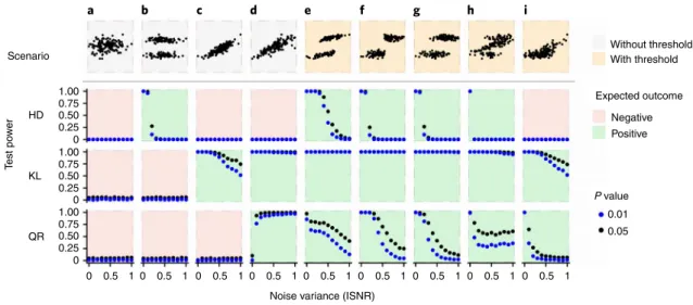
ideal data without random variation around the response magni- tude (scenarios g–i in Fig. 2), with the exception of the unlikely case that all systems are characterized by the same threshold (scenario f in Fig. 2). For HD, the power collapses completely with only mod- erate noise levels (Fig. 2). Only KL is still able to detect changes in response magnitude with increasing pressure with increasing variance, either around gradual shifts in response magnitude (sce- narios c and d in Fig. 2) or around thresholds (scenarios e–i). The simulations corroborate our general empirical finding across the 36 datasets that thresholds are rarely detectable in data even if using statistical methods developed for threshold detection.
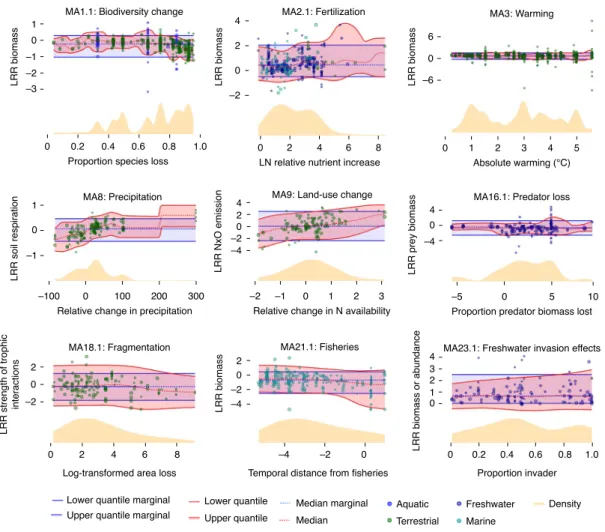
Even when thresholds were empirically detected, limited infer- ence can be made as shown by highlighting several individual meta-analysis datasets to illustrate specific ecosystem responses to particular environmental pressures. The first meta-analysis in our dataset (MA1.1) exemplifies the general results. The overall response of biomass production to biodiversity loss tended to be negative and became more negative for larger proportions of species lost without changes in the variational range of effect sizes (Fig. 3).
This gradual response type was also found in the analysis of fertil- ization effects on biomass production (MA2.1) and in soil responses to changes in precipitation (MA8) and land-use change (MA9) as well as prey responses to predator loss (MA16.1). Ten additional examples of this type of response involving other drivers of environ- mental change are provided in the supporting material (Extended Data Fig. 2 and Supplementary Table 1). In all of these cases, the magnitude of the environmental change altered the magnitude of the response—as expected—but the variance around this relation- ship did not indicate the emergence of a ‘novel’ ecosystem response beyond a pressure threshold. Eight cases showed significant QR tests, of which three showed an increase in response variance only at highest pressure strength and two cases showed a reduction in
response variance with increasing pressure. Thus, only three out of 36 cases showed a shifting distribution of effect sizes with increas- ing pressure that was consistent with the emergence of new types of responses above a threshold. These comprise land-use change effects on mammal abundance (MA6.5), warming effects on corals (MA10) and fertilization effects on microbial respiration (MA17.2;
all Extended Data Fig. 2). By contrast, in 12 of the 36 meta-analyses, neither KL nor QR were significant (exemplified by MA23.1 in Fig. 3;
for others see Extended Data Fig. 2), indicating that no increases in response magnitudes or threshold trangressions were observed.
These results are relevant for across-system analyses of single pressure gradients but in many cases management might not have a-priori knowledge of which pressure gradient leads to transgres- sions. To analyse this situation, we further aggregated our analysis across drivers, organism groups and ecosystems, by standardiz- ing and normalizing the pressure gradient to a median of 0 and a range of –1 to 1 (Fig. 4). The range of responses was impressive, the effect sizes in cases indicated >200-fold increase or decrease in the measured ecosystem variable (Fig. 4a). Both KL and QR tests were highly significant for the aggregated data, indicating a strong impact of pressure intensity on the strength and variance of the ecologi- cal response (Supplementary Table 1). However, this increase in the variance of effect sizes was found for studies with normalized pres- sures >0.5, which comprised the top 3.5% of the manipulated range of potential impacts (Fig. 4b). This observation resembles a ‘sledge- hammer effect’; that is, system transformation by huge impact, which is a trivial consequence of the large pressure magnitude and the complete transformation of the system.
As the sign of the effect size depends upon the specific associa- tion of driver and effect in each meta-analysis, we also analysed the absolute magnitude of response (|LRR|) independent of sign for the aggregated dataset (Fig. 4c). We found that the median |LRR|
Scenario
1.00 0.75 0.50 0.25 0 1.00 0.75 0.50 0.25 0 1.00 0.75 0.50 0.25 0
0 0.5 1 0 0.5 1 0 0.5 1 0 0.5 1 0
Noise variance (ISNR)
0.5 1 0 0.5 1 0 0.5 1 0 0.5 1 0 0.5 1 HD
KL
QR
Test power
a b c d e f g h i
Without threshold
Negative Positive
0.01 0.05
With threshold Expected outcome
P value
Fig. 2 | Detection probability for thresholds in global change experiments using kernel density estimation. We analysed the test power for nine scenarios of responses to pressure in meta-analyses. The derivation of each scenario is described in the Supplementary Text and Extended Data Fig. 3, the top panel presents an illustration of each scenario (full description in Extended Data Fig. 3). Each scenario is represented in a column, the test power is then given for each of the three statistical tests used in our analyses (HD, Hartigan’s dip test; KL, Kullback–Leibler; QR, quantile ratio). a–d, These scenarios do not comprise a threshold, where the scenario shown in a is the null model without an effect of the pressure on the response. e–i, These scenarios do comprise a threshold, for the last two combined with intermediate responses. For the three statistical tests used in our analyses, the expected outcome is colour-coded, with green representing that the test should be significant. Test power is given as the proportion of 1,000 simulated datasets for which the tests were significant with a probability P = 0.05 (black) and P = 0.01 (blue) along a gradient of increasing noise variance (inverse signal-to-noise ratio, ISNR). Bandwidth selection was based on the ‘solve-the-equation’ method of Sheather and Jones59. The estimated bandwidth was adjusted by a factor of 2.5 in each case because this optimized test power for all cases. The three tests together allow perfect detection of thresholds in the absence of noise (e–h). If threshold-type and gradual responses are mixed (i), the analysis of multimodality (HD) is no longer able to pick up the threshold embedded in the data, as the simultaneous increase in mean and variance of the response (as in d) masks modes in the response distribution. With increasing noise variance, however, the detection probability for thresholds via HD and QR rapidly decrease.
Articles NaTuRE Ecology & EvoluTIoN
increased with increasing environmental pressure, as did the vari- ance, particularly so at the highest pressure magnitudes (significant KL and QR tests; Supplementary Table 1). The median |LRR| cor- responded to 1.5–2-fold increases or decreases in process rates or properties, whereas the range of responses (the 5–95% quantiles of |LRR|) exceeded fivefold changes even at the smallest pressure strengths. Thus, even at very small pressures, very large responses can occur.
Discussion
Analysis of the 4,601 experiments that we assembled here, poten- tially the most comprehensive data available, did not enable us to estimate where thresholds might have been crossed. Instead, the data suggest that the ecosystem impacts of human-induced changes in environmental drivers are better characterized by gradual shifts in response magnitudes with increasing pressure coupled with broad variations around this trend. While our analyses do not rule out the existence of tipping points, they bring into question the utility of threshold-based concepts in management and policy if we cannot detect thresholds in nature
10,11. Expectation of threshold responses ultimately leads to an underestimation of the large conse- quences of small environmental pressures
12. Moreover, it marginal- izes the importance of other, more complex, nonlinear dynamics under global change, which may underlie the considerable variance around gradually increasing response magnitudes.
Our use of field and seminatural experiments has the advan- tage that these often involve pressures that are larger than observed environmental conditions, as they commonly incorporate future scenarios of severe environmental change
13. This counters the argu- ment that thresholds exist but have not yet been reached. Still, some caveats to our approach need to be acknowledged. First, the absence of evidence is obviously not the evidence of absence: as shown by our explicit analysis of test power, the existence of thresholds can be masked by high interstudy variance (especially for HD). However, this also questions the usefulness of thresholds if their occurrence is dependent on the complex interaction of multiple pressures and their detection is only possible under very high signal-to-noise ratios. Without a-priori knowledge across specific systems of when thresholds might appear, any definition of thresholds—even if pre- cautionary principles are used—must remain arbitrary. Second, we focused on functional, not compositional, aspects of ecosys- tems and do not make conclusions about threshold pressures for changes in composition. However, compositional and functional stability often show interdependencies
14because compensatory dynamics between species may dampen the response in ecosystem functions
15or allow for rapid recovery from a phase shift
16–18. Given that the functions addressed here often are aggregate properties of the communities investigated, we thus consider it unlikely that thresholds are more prevalent for compositional responses. Third, the temporal extent of the experimental studies in our database is
1
–1 –2 –3 0
LRR biomass LRR biomass LRR biomass
4 2 0 –2
MA1.1: Biodiversity change MA2.1: Fertilization MA3: Warming
6 0 –6
0 0.2 0.4
Proportion species loss
0.6 0.8 1.0 0 2 4
LN relative nutrient increase
6 8 0 1 2 3 4 5
Absolute warming (°C)
1 0 –1
LRR soil respiration
MA8: Precipitation
–100 0 100
Relative change in precipitation
200 300
42
–2–4 0
LRR NxO emission
–2 –1 0
Relative change in N availability
1 2 3
4 –4 0
LRR prey biomass
MA9: Land-use change MA16.1: Predator loss
–5 0 5 10
Proportion predator biomass lost
2 0 –2 LRR strength of trophic interactions
0 2 4 6 8
Log-transformed area loss MA18.1: Fragmentation
2 –2 –4 0
LRR biomass
MA21.1: Fisheries
–4 –2 0
Temporal distance from fisheries 43 21 0
LRR biomass or abundance 0 0.2 0.4 0.6 0.8 1.0
Proportion invader MA23.1: Freshwater invasion effects
Lower quantile marginal
Upper quantile marginal Lower quantile Upper quantile
Median marginal Median
Aquatic
Terrestrial Marine
Freshwater Density
Fig. 3 | example meta-analyses testing for changes in the response magnitude along with increasing pressure intensity. Red- and blue-shaded regions indicate the (5–95%) interquantile ranges for, respectively, the bivariate data (including the pressure gradient) and the marginal distribution of LRR (integrating out the pressure gradient). Dashed red and thick blue lines trace the related median (50% quantile). Overlain are the data points and, at the bottom, the yellow-shaded area indicates the distribution of stressor variables resulting from a weighted kernel density estimation. Circle size reflects statistical weight. The suggestive break in the responses in MA8 is induced by a lack of data covering intermediate pressure magnitude. LN, natural log.
Articles
NaTuRE Ecology & EvoluTIoN
limited; it rarely exceeds the scale of tens of generations of organ- isms. However, there is no strong support for why threshold trans- gressions should increase through time. Threshold-related concepts thus would be untestable in ecology, as their absence could always be ascribed to insufficiently long observation periods.
The lack of clearly defined and generally applicable thresholds distinguishing between tolerable and non-tolerable responses has obvious implications for environmental policies. The use of thresh- olds has been critically discussed in ecosystem management, con- servation and restoration
19–21to establish precautionary principles for environmental policy. Using such threshold arguments in a world where changes are too case-specific and variable to allow prediction of tipping points undermines this precautionary argu- ment. It leads to the anticipation of major system transformation as thresholds are passed, whereas most observed responses to envi- ronmental change represent progressively shifting baselines on timescales of human perceptions
22,23. Consequently, environmental concerns might appear overstated if thresholds are taken for the general case but critical transitions associated with transgressing thresholds are not observed
24,25. The frequently major and highly variable responses we observed even at low pressure magnitudes indicate that safe-operating spaces are unlikely to be definable from data. The data resonate well with the fact that, conceptually, thresh- olds occur under special and limiting conditions. Our results thus question the pervasive presence of threshold concepts in manage- ment and policy.
Methods
Data. We searched the ISI Web of Science (WoS) using a search string targeted towards detecting meta-analyses in a global change context (Topic: [‘metaanalysis’
or ‘meta-analysis’ or ‘metaanalyses’ or ‘meta-analyses’] AND Topic: [‘global change’ or ‘fertili*’ or ‘land-use’ or ‘acidification’ or ‘warming’ or ‘temperature’
or ‘eutrophication’ or ‘disturbance’ or ‘invasion’ or ‘extinction’ or ‘drought’ or
‘ultraviolet’] AND Topic: [‘chang*’ or ‘manipulation*’ or ‘experim*’ or ‘treatm*’]).
We refined the results by focusing on the WoS research area ‘Environmental sciences and ecology’. This search (done on 11 September 2016) yielded 979 studies from which most did not fit all of our inclusion criteria (upon request, we can provide a list of all studies with the study-specific criteria to include or exclude), which were as follows:
• The paper provided a formal meta-analysis with effect sizes, which quantified the responses to a factor that represented a global change impact. The factor was either an experimental treatment or an in-situ change. This excluded numerous studies that were verbal/vote-counting reviews or provided effect sizes as a response to non-global-change factors (for example, mitigation efforts).
• The response was measured at the level of ecological communities or eco- systems. This excluded studies where responses were measured at the level of single species, as these were deemed inappropriate to detect regime shifts, or at the level of human societies (for example, health aspects and economy).
We also excluded fossil data as not being affected by anthropogenic global change and non-biological response variables (for example, the effect of CO2-enrichment on water pH).
• Given that effect sizes on species richness have recently been criticized strongly for being statistically biased26, we decided not to use biodiversity response variables but only functional processes or properties at the commu- nity or ecosystem level (details below). As we explicitly address the statistical distribution of effect sizes (see below), this statistical bias was considered to be potentially misleading in the context of our analysis. However, we used cases where biodiversity loss was the manipulated component of global change and a functional response was measured.
From the remaining 162 meta-analyses that fulfilled these criteria, we extracted the information needed to perform our analyses. This included a measure of the magnitude of the stressor (impact, driver) and the effect size as well as its sampling variance or weight (response). When the information was not given in an online appendix or associated data table, we contacted the authors to ask for data access.
Still, we had to exclude further meta-analyses, as they: did not quantify the stressor magnitude (this was especially common in meta-analyses addressing the response to invasive species); did not contain enough cases to perform analysis (we set the critical number of effect sizes to 35 as a minimum to detect variance shifts);
overlapped with other meta-analyses on the same subject (this was especially found for analyses on eutrophication and biodiversity loss, where we always opted for the most consistent and information-dense alternative); did not provide available data.
The final database contained 24 meta-analyses (information derived from 29 papers27–55), which were divided into 36 cases (Supplementary Table 1). Subsetting multiple cases from a meta-analysis was done if different drivers were tested or different response categories were used in a single meta-analysis. We followed the authors in defining response categories and stressor variables. We excluded laboratory experiments and focused our study solely on field experiments and observational studies. The resulting dataset reflects ecological responses in the 12
6 0 –6 –12 log response ratio log response ratiolog response ratiox-densityx-densityx-density
Normalized environmental pressures
Normalized environmental pressures
Normalized environmental pressures
y-density
y-density
y-density 3
2 1 0 –1 –2 –3
3 2
1
0
Lower quantile marginal Upper quantile marginal
Lower quantile Upper quantile Median marginal
Median Freshwater Marine
Aquatic Terrestrial
x-density y-density
a
b
c
Fig. 4 | Analysis of aggregate data across meta-analyses. a, LRR of ecological processes across a gradient of environmental change, where the different pressures were normalized to a median of 0 and a range of
−1 to 1. Circle size reflects statistical weight. Shaded regions indicate the interquantile (5–95%) ranges for the marginal distribution (blue) and the bivariate distribution (red). Density of values along the stressor and the response axis are given below (yellow) or at the right margin (green), respectively. b, Same as a but without single effect sizes, focusing on the distribution of response magnitudes over the normalized pressure gradient.
c, Same as b but for absolute response magnitudes. Note the change in scale of the y axis in the three panels.
Articles NaTuRE Ecology & EvoluTIoN
form of ecosystem processes (primary or secondary production, feeding rates and element fluxes) to the most pervasive anthropogenic alterations of our planet (Supplementary Table 1).
Statistical approach. For each meta-analysis dataset containing a measure of the stressor magnitude (X), the response variable (log response ratio, LRR) and its sampling variance (var.LRR), we assessed whether the dataset reflects any statistically significant influence of the stressor variable on the response. As the data basis of each meta-analysis (and thus the sources of variation of LRR within each dataset) is unknown to us, we devised three robust non-parametric test statistics and assessed their statistical significance by permutation tests.
An averaged KL divergence quantified the overall deviation between the response distribution for a given stressor value and the marginal response distribution (that is, the response distribution when collapsing all response data onto a single axis ignoring the stressor variable). Second, a quantile ratio (QR) of interquantile range (95–5%) was then used to quantify substantial variability of the response distribution width across the range of observed stressors. Finally, we used the HD test to assess the multimodality of effect sizes9. Based on simulation-based P values, HD provides a narrow test for the case of bi-(multi)-stability of responses, analogous to the bimodality test proposed by Scheffer and Carpenter56. A significant HD indicates that the responses along the pressure gradient fall into two (or more) clearly separated categories, which indicates the presence of two (or more) alternative ecosystem states. Essentially, strict bimodality across a wide range of studies is a rather narrow expectation but we include this test as the bifurcation case is the one most often discussed in considerations of thresholds, tipping points and regime shifts56,57.
For both KL and QR, the assessment of statistical significance was done by a permutation test: the null hypothesis (NH) that the response distribution is unrelated to the stressor is simulated by breaking up paired variables (X, LRR, var.LRR) and recombining them in the form (X′, LRR, var.LRR), where X′ is a permutation of recorded stressor values. If the NH were valid, this permutation should induce no substantial difference. Computing the two test statistics (KL and QR) for the permuted dataset (X′, LRR, var.LRR) and repeating these steps 10,000 times generates the distribution of the test statistics under validity of the NH and allows extraction of a P value as the fraction of permutations that yielded a similar or larger value for the test statistic (KL or QR) as the original dataset (X, LRR, var.LRR).
In comparison to alternative approaches, our methods are robust and non-parametric—they do not rely on functional assumptions and use only the supposed smoothness of a possible connection between stressor and response.
Reconstructing the NH by simulating surrogate data guarantees perfect control of errors of the first kind (false positive statements) and even would handle a constant bias of estimators. Given the breadth of underlying meta-analyses, we also consider our analysis highly conservative with regard to publication bias and study selection.
Finally, using a weighted approach downgrades the influence of studies with very high internal variance and thus decreases the chance of missing threshold-like responses because of too-noisy data (false negative statements).
It should be noted that neither the single experiments summarized in each meta-analysis nor the meta-analyses themselves were designed to detect thresholds. The inclusion of studies not necessarily looking for thresholds actually reduces the risk of publication bias towards positive results. However, even if the underlying experiments were not planned to detect thresholds, our statistical approach should reveal these if they fall into the covered range of stressors, which can be expected as this range encompasses stressor magnitudes not yet experienced under realistic conditions.
Statistical analyses. For each effect size in each meta-analysis, a statistical weight is assigned to each data point as the log-transformed inverse sampling variance of the effect size
log 1þ 1 var:LRR
ð1Þ As described above, surrogate datasets (reflecting the NH) are created by permuting the list of stressor values in X (yielding X′ = X shuffled). From the list of stressor values, a smooth probability distribution PX(gx) is computed via weighted (with statistical weights calculated following equation (1)) kernel density estimation (with a Gaussian kernel and an optimized bandwidth, compare Simulations) for grid points gx that span the range of observed stressor values (Extended Data Fig. 4). A smooth density surface over the grid (gx, gy) in the (X, LRR) plane is computed from the dataset (and the surrogates) via a two-dimensional weighted (with statistical weights calculated following equation (1)) kernel density estimation (bivariate Gaussian D-class kernel with optimized bandwidth) (Extended Data Fig. 5). For each grid point gx, the density profile along gy is converted to a conditional probability distribution PLRR|X(gy|gx) by normalization (Extended Data Fig. 6, with results for the original data and the surrogate data). Based on the conditional cumulative distribution function,
FLRRjXðgyjgxÞ ¼ X
gy0≤gy
PLRRjXX
PLRRjXðgy0jgxÞ ð2Þ
(Extended Data Fig. 7), the 5%, 50% (median) and 95% quantiles can be extracted for each grid point gx (Extended Data Fig. 8). The test statistics that we devised are:
1. the average KL divergence KL¼X
gx
PXð Þgx X
gy
PLRRjXðgyjgxÞlogPLRRjXðgyjgxÞ
PLRRð Þgy ð3Þ that shares the useful property of being non-negative and that vanishes if, and only if, PLRR|X≡ PLRR (almost everywhere). Pronounced differences between the two empirical distributions are thus condensed in values substantially larger than zero.
2. the quantile ratio (QR) of interquantile (5–95%) ranges (IQR) QR¼IQR955ð99%Þ
IQR955ð1%Þ ð4Þ where IQR955ð Þqx
I denotes the qx-quantile of the 5–95% interquantile range of the conditional probability distribution PLRR|X(gy|gx) and the subsequent percentage in brackets indicates the related weighted quantile across the stressor grid points. We choose this latter definition for robustness, rather than the maximum/minimum ratio which may be prone to distortions by extremes. This measure was devised to indicate substantial changes of the LRR variance along the stressor axis.
3. the HD statistic tests for multimodality, which, if significant, indicates that a frequency distribution has more than one mode.
Values of all test statistics obtained for the original dataset were assessed for statistical significance. This was done by excessively repeating the permutation strategy to create surrogate data in accordance with the NH of a non-existent connection between stressor X and response LRR. P values for both test statistics (KL and QR) were obtained as fractions of 10,000 surrogate sets (in the case of HD, 2,000 permutations), leading to test statistics exceeding related values of the original dataset.
In addition to the employed kernel density estimates generating cumulative distribution functions and derived quantiles, we used a nonlinear quantile regression supplied by the R package qgam58. This package is based on general additive models and returns quantiles instead of standard mean response. With qgam we estimated the following quantiles: 0.001, 0.1, 0.2, 0.3, 0.4, 0.5, 0.6, 0.7, 0.8, 0.9 and 0.999. Because these quantile curves were computed sequentially, independently resultant lines could intersect. To resolve this problem, we used the R package cobs to perform a penalized B-spline regression of obtained quantiles (separately for every grid point gx), bound to the constraint of a monotonic increase, thus yielding a smooth cumulative distribution function. As for the kernel density estimation, exemplary 5%, 50% (median) and 95% quantiles are shown in Extended Data Fig. 8.
Under default settings, the qgam routine was very time consuming and, in comparison with the bandwidth optimized kernel density method, had inferior test power (Fig. 2 and Supplementary Table 1). This may be due to the fact that, because of excessive run time an optimization of qgam parameters was not feasible. We therefore constrain reporting of our results to those obtained with the optimized kernel density method.
Simulations. We examined the performance of our tests by simulating artificial datasets that combined nine deterministic backbone structures with additive noise (normally distributed random fluctuations) of controlled intensity. The deterministic backbone structures were chosen to reflect a broad range of scenarios. The noise intensity is quantified via the inverse signal-to-noise ratio (ISNR), that is the size ratio of fluctuations and backbone structure. The nine cases are depicted in Extended Data Fig. 3, each for small (ISNR = 0.05) and large (ISNR = 0.95) noise intensity. In Fig. 2 and Supplementary Table 1, we list the expected outcome of the three designed tests for the noise-free case. To assess the performance of the tests under various noise conditions, we simulated, for each ISNR value (in the range [0–1]), 1,000 artificial datasets and collected related test decisions (for two decision criteria P = 0.05 and 0.01 and all three tests). In the case of an expected positive test, the fraction of positive test decisions thus estimates the test power (1-error of the second kind). We note that simulations of the test power were also underlying the optimization of the kernel bandwidth, where bandwidth selection was based on the ‘solve-the-equation’ method of Sheather and Jones59.
In all simulated cases with small to moderate noise (ISNR < 0.5), threshold structures in simulated response–stressor relations could be detected with high reliability (at least for the KL and QR tests). Of course, for strong noise (ISNR ≥ 1), thresholds may be masked by random fluctuations reflecting natural variability.
In such situations, the underlying threshold structure, although present, will no longer be ecologically relevant because it is overridden by natural variability.
Reporting Summary. Further information on research design is available in the Nature Research Reporting Summary linked to this article.
Data availability
All data are available at https://zenodo.org/record/3828869#.XsI4ZmgzaUk.
Articles
NaTuRE Ecology & EvoluTIoN
code availability
All code are available at https://zenodo.org/record/3828869#.XsI4ZmgzaUk.
Received: 21 January 2020; Accepted: 15 June 2020;
Published: xx xx xxxx
References
1. Scheffer, M., Carpenter, S., Foley, J. A., Folke, C. & Walker, B. Catastrophic shifts in ecosystems. Nature 413, 591–596 (2001).
2. Scheffer, M. Critical Transitions in Nature and Society (Princeton Univ.
Press, 2009).
3. Rockström, J. et al. A safe operating space for humanity. Nature 461, 472–475 (2009).
4. Folke, C. et al. Regime shifts, resilience and biodiversity in ecosystem management. Annu. Rev. Ecol. Evol. Syst. 35, 557–581 (2004).
5. Donohue, I. et al. Navigating the complexity of ecological stability. Ecol. Lett.
19, 1172–1185 (2016).
6. Aichi Biodiversity Targets (UN, 2010); https://www.cbd.int/sp/targets/
7. Carpenter, S. R. & Brock, W. A. Rising variance: a leading indicator of ecological transition. Ecol. Lett. 9, 308–315 (2006).
8. Scheffer, M. et al. Early-warning signals for critical transitions. Nature 461, 53–59 (2009).
9. Hartigan, J. A. & Hartigan, P. M. The dip test of unimodality. Ann. Stat. 13, 70–84 (1985).
10. Montoya, J. M., Donohue, I. & Pimm, S. L. Planetary boundaries for biodiversity: implausible science, pernicious policies. Trends Ecol. Evol. 33, 71–73 (2018).
11. Pimm, S. L., Donohue, I., Montoya, J. M. & Loreau, M. Measuring resilience is essential to understand it. Nat. Sustain. 2, 895–897 (2019).
12. Clark, C. M. & Tilman, D. Loss of plant species after chronic low-level nitrogen deposition to prairie grasslands. Nature 451, 712–715 (2008).
13. Korell, L., Auge, H., Chase, J. M., Harpole, W. S. & Knight, T. M. We need more realistic climate change experiments for understanding ecosystems of the future. Glob. Change Biol. 26, 325–327 (2020).
14. Hillebrand, H. et al. Decomposing multiple dimensions of stability in global change experiments. Ecol. Lett. 21, 21–30 (2018).
15. Connell, S. D. & Ghedini, G. Resisting regime-shifts: the stabilising effect of compensatory processes. Trends Ecol. Evol. 30, 513–515 (2015).
16. Bruno, J. F., Sweatman, H., Precht, W. F., Selig, E. R. & Schutte, V. G. W.
Assessing evidence of phase shifts from coral to macroalgal dominance on coral reefs. Ecology 90, 1478–1484 (2009).
17. Diaz-Pulido, G. et al. Doom and boom on a resilient reef: climate change, algal overgrowth and coral recovery. PLoS ONE 4, e5239 (2009).
18. Carpenter, S. R. et al. Early warnings of regime shifts: a whole-ecosystem experiment. Science 332, 1079–1082 (2011).
19. Suding, K. N. & Hobbs, R. J. Threshold models in restoration and conservation: a developing framework. Trends Ecol. Evol. 24, 271–279 (2009).
20. Vaquer-Sunyer, R. & Duarte, C. M. Thresholds of hypoxia for marine biodiversity. Proc. Natl Acad. Sci. USA 105, 15452–15457 (2008).
21. Groffman, P. M. et al. Ecological thresholds: the key to successful environmental management or an important concept with no practical application? Ecosystems 9, 1–13 (2006).
22. Hughes, T. P., Carpenter, S., Rockstrom, J., Scheffer, M. & Walker, B. Multiscale regime shifts and planetary boundaries. Trends Ecol. Evol. 28, 389–395 (2013).
23. Papworth, S. K., Rist, J., Coad, L. & Milner-Gulland, E. J. Evidence for shifting baseline syndrome in conservation. Conserv. Lett. 2, 93–100 (2009).
24. Schlesinger, W. H. Planetary boundaries: thresholds risk prolonged degradation. Nat. Clim. Change 1, 112–113 (2009).
25. Duarte, C. M. et al. Reconsidering ocean calamities. BioScience 65, 130–139 (2015).
26. Chase, J. M. & Knight, T. M. Scale-dependent effect sizes of ecological drivers on biodiversity: why standardised sampling is not enough. Ecol. Lett. 16, 17–26 (2013).
27. Cardinale, B. J. et al. Effects of biodiversity on the functioning of trophic groups and ecosystems. Nature 443, 989–992 (2006).
28. Gruner, D. S. et al. A cross-system synthesis of consumer and nutrient resource control on producer biomass. Ecol. Lett. 11, 740–755 (2008).
29. Elser, J. J. et al. Global analysis of nitrogen and phosphorus limitation of primary producers in freshwater, marine and terrestrial ecosystems. Ecol. Lett.
10, 1135–1142 (2007).
30. Lin, D., Xia, J. & Wan, S. Climate warming and biomass accumulation of terrestrial plants: a meta-analysis. New Phytol. 188, 187–198 (2010).
31. Treseder, K. K. Nitrogen additions and microbial biomass: a meta-analysis of ecosystem studies. Ecol. Lett. 11, 1111–1120 (2008).
32. Akiyama, H., Yan, X. & Yagi, K. Evaluation of effectiveness of enhanced-efficiency fertilizers as mitigation options for N2O and NO emissions from agricultural soils: meta-analysis. Glob. Change Biol. 16, 1837–1846 (2010).
33. Gibson, L. et al. Primary forests are irreplaceable for sustaining tropical biodiversity. Nature 478, 378–381 (2011).
34. Liang, J. Y., Qi, X., Souza, L. & Luo, Y. Q. Processes regulating progressive nitrogen limitation under elevated carbon dioxide: a meta-analysis.
Biogeosciences 13, 2689–2699 (2016).
35. Liu, L. L. et al. A cross-biome synthesis of soil respiration and its determinants under simulated precipitation changes. Glob. Change Biol. 22, 1394–1405 (2016).
36. van Lent, J., Hergoualc’h, K. & Verchot, L. V. Reviews and syntheses: soil N2O and NO emissions from land use and land-use change in the tropics and subtropics: a meta-analysis. Biogeosciences 12, 7299–7313 (2015).
37. Ateweberhan, M. & McClanahan, T. R. Relationship between historical sea-surface temperature variability and climate change-induced coral mortality in the western Indian Ocean. Mar. Pollut. Bull. 60, 964–970 (2010).
38. Gärtner, M. et al. Invasive plants as drivers of regime shifts: identifying high-priority invaders that alter feedback relationships. Divers. Distrib. 20, 733–744 (2014).
39. Dooley, S. R. & Treseder, K. K. The effect of fire on microbial biomass: a meta-analysis of field studies. Biogeochemistry 109, 49–61 (2012).
40. Dijkstra, F. A. & Adams, M. A. Fire eases imbalances of nitrogen and phosphorus in woody plants. Ecosystems 18, 769–779 (2015).
41. Lu, M. et al. Responses of ecosystem carbon cycle to experimental warming:
a meta-analysis. Ecology 94, 726–738 (2013).
42. Griffin, J. N., Byrnes, J. E. K. & Cardinale, B. J. Effects of predator richness on prey suppression: a meta-analysis. Ecology 94, 2180–2187 (2013).
43. Srivastava, D. S. et al. Diversity has stronger top-down than bottom-up effects on decomposition. Ecology 90, 1073–1083 (2009).
44. Östman, Ö. et al. Top-down control as important as nutrient enrichment for eutrophication effects in North Atlantic coastal ecosystems. J. Appl. Ecol. 53, 1138–1147 (2016).
45. Katano, I., Doi, H., Eriksson, B. K. & Hillebrand, H. A cross-system meta-analysis reveals coupled predation effects on prey biomass and diversity.
Oikos 124, 1427–1435 (2015).
46. Borer, E. T. et al. What determines the strength of a trophic cascade? Ecology 86, 528–537 (2005).
47. Hodapp, D. & Hillebrand, H. Effect of consumer loss on resource removal depends on species-specific traits. Ecosphere 8, e01742 (2017).
48. Liu, L. L. & Greaver, T. L. A global perspective on belowground carbon dynamics under nitrogen enrichment. Ecol. Lett. 13, 819–828 (2010).
49. Martinson, H. M. & Fagan, W. F. Trophic disruption: a meta-analysis of how habitat fragmentation affects resource consumption in terrestrial arthropod systems. Ecol. Lett. 17, 1178–1189 (2014).
50. Holden, S. & Treseder, K. A meta-analysis of soil microbial biomass responses to forest disturbances. Front. Microbiol. 4, 163 (2013).
51. Nagelkerken, I. & Connell, S. D. Global alteration of ocean ecosystem functioning due to increasing human CO2 emissions. Proc. Natl Acad. Sci.
USA 112, 13272–13277 (2015).
52. Kaiser, M. J. et al. Global analysis of response and recovery of benthic biota to fishing. Mar. Ecol. Prog. Ser. 311, 1–14 (2006).
53. Gill, D. A. et al. Capacity shortfalls hinder the performance of marine protected areas globally. Nature 534, 665–669 (2017).
54. Gallardo, B., Clavero, M., Sánchez, M. I. & Vilà, M. Global ecological impacts of invasive species in aquatic ecosystems. Glob. Change Biol. 22, 151–163 (2016).
55. Vila, M. et al. Ecological impacts of invasive alien plants: a meta-analysis of their effects on species, communities and ecosystems. Ecol. Lett. 14, 702–708 (2011).
56. Scheffer, M. & Carpenter, S. R. Catastrophic regime shifts in ecosystems:
linking theory to observation. Trends Ecol. Evol. 18, 648–656 (2003).
57. Andersen, T., Carstensen, J., Hernandez-Garcia, E. & Duarte, C. M.
Ecological thresholds and regime shifts: approaches to identification. Trends Ecol. Evol. 24, 49–57 (2009).
58. Fasiolo, M., Goude, Y., Nedellec, R. & Wood, S. N. Fast calibrated additive quantile regression. J. Am. Stat. Assoc. https://doi.org/10.1080/01621459.2020.
1725521 (2020).
59. Sheather, S. J. & Jones, M. C. A reliable data-based bandwidth selection method for kernel density estimation. J. Royal Stat. Soc. B 53, 683–690 (1991).
Acknowledgements
The data reported in this paper are presented and derived from 36 different meta-analyses; they are archived and available from each of these as indicated in the Supplementary Text. The concept of this paper emerged during scientific discussions with T. Blenckner at Stockholm University, at the UK NERC/BESS Tansley Working Group on ecological stability and the TippingPond EU Biodiversa project. The actual work was funded by the Lower Saxony Ministry of Science and Culture through the MARBAS project to H.H. and the HIFMB, a collaboration between the Alfred-Wegener-Institute, Helmholtz-Center for Polar and Marine Research and the Carl von Ossietzky University Oldenburg, initially funded by the Ministry for Science and
Articles NaTuRE Ecology & EvoluTIoN
Culture of Lower Saxony and the Volkswagen Foundation through the ‘Niedersächsisches Vorab’ grant programme (grant no. ZN3285). The work was finalized with support by Deutsche Forschungsgemeinschaft grant no. HI848/26–1. L. Toaspern helped with gathering data from invasion meta-analyses. P. Ruckdeschel helped with the statistical approach. M. Vilà provided additional information on their published meta-analyses. We acknowledge the comments by U. Feudel, G. Gerlach and the members of the Plankton Ecology Lab at the Carl von Ossietzky University Oldenburg on the manuscript which helped with our argumentation.
Author contributions
H.H. designed the analysis and discussed the framework with I.D. J.M.M., J.A.F. and J.M. developed the statistical approach with input from H.H. and D.H. H.H. assembled the effect size information. J.A.F. and J.M. performed the statistical analysis. M.K., A.M.L. and W.S.H. provided input on palaeoecological and experimental constraints, respectively. H.H. wrote the manuscript together with W.S.H. and J.M.M. as well as input from all co-authors.
competing interests
The authors declare no competing interests.
Additional information
Extended data is available for this paper at https://doi.org/10.1038/s41559-020-1256-9.
Supplementary information is available for this paper at https://doi.org/10.1038/
s41559-020-1256-9.
Correspondence and requests for materials should be addressed to H.H.
Peer review information Peer reviewer reports are available.
Reprints and permissions information is available at www.nature.com/reprints.
Publisher’s note Springer Nature remains neutral with regard to jurisdictional claims in published maps and institutional affiliations.
© The Author(s), under exclusive licence to Springer Nature Limited 2020
Articles
NaTuRE Ecology & EvoluTIoN Articles
NaTuRE Ecology & EvoluTIoN
Extended Data Fig. 1 | Test power as in Fig. 2, but for the “qgam” approach. Fractions of positive test results (equals test power when test should be positive) for simulated test cases. We analysed the test power for 9 scenarios of responses to pressure in meta-analyses, the derivation of each scenario is described in the supplementary online material, Extended Data Fig. 7. Scenarios a–d do not comprise a threshold, where scenario a is the null model without an effect of the pressure on the response. Scenarios e–i do comprise a threshold, for the latter two combined with intermediate responses. For the three statistical test used in our analyses, the expected outcome is colour-coded, with green representing that the test should be significant. We then tested the proportion of 1000 simulated datasets for which the tests were significant with a probability p = 0.05 (black) and p = 0.01 (blue). We did for increasing noise variance (= inverse signal-to-noise ratio). The three tests together allow perfect detection of thresholds at the absence of noise (scenarios e–h), only if threshold-type and gradual responses are mixed (scenario i), the analysis of multimodality (HD) fails, giving the same output as a gradual increase in mean and variance of the response (scenario d). With increasing noise variance, however, the detection probability for thresholds via HD and QR rapidly decreases.We used default settings for the “qgam” approach due to high runtimes and computational effort, thus settings are not optimized as for the test power calculations based on kernel density estimation. Note: HD is equal to kernel method, because it is not based on different quantile estimations.
Articles NaTuRE Ecology & EvoluTIoN
Articles NaTuRE Ecology & EvoluTIoN
Extended Data Fig. 2 | See next page for caption.
Articles
NaTuRE Ecology & EvoluTIoN Articles
NaTuRE Ecology & EvoluTIoN
Extended Data Fig. 2 | changes in the response magnitude along increasing pressure strength. Further meta-analyses testing for changes in the response magnitude along increasing pressure strength. Red and blue shaded regions indicate the (5%-95%) interquantile ranges for the bivariate data (including the pressure gradient) and the univariate LRR data (ignoring the pressure gradient = homogeneous marginal probability), respectively. Solid red and dashed blue thick lines trace the related median (50% quantile). Overlain are the data points and at the bottom the yellow shaded area indicates the distribution px(gx) resultant from a weighted kernel density estimation. Colour codes for habitat (dark blue: freshwater, aquamarine: marine, green:
terrestrial), circle size reflect statistical weight.
Articles NaTuRE Ecology & EvoluTIoN
Articles NaTuRE Ecology & EvoluTIoN
Extended Data Fig. 3 | See next page for caption.
Articles
NaTuRE Ecology & EvoluTIoN Articles
NaTuRE Ecology & EvoluTIoN
Extended Data Fig. 3 | Test cases at different noise levels. In order to assess the power of our statistical tests, we simulated artificial meta-analyses combining prototypical response~stressor relationships with (normally distributed) random fluctuations reflecting natural variability, and compared related statistical test results with expectations. Stressor range (along horizontal range) and deterministic effect sizes (along vertical axis) are normalized to [−0.5,0.5] x [0.5,0.5]. Stressor values are normally distributed with mean zero. The relative intensity of random fluctuations is quantified by inverse signal-to-noise ratio (isnr). A grey background indicates absence of thresholds, yellow background threshold presence. a, (neutral -simple-): Here pressure strength has no impact on the response, which falls into a single response. Thus, we assume that across all “studies” in this “meta-analysis”, there is one main response type and no threshold. b, (neutral -bimodal-): Here pressure strength has no impact on the response, which falls into either of two alternative attractors: a weak and a strong response. Thus, we assume that across all “studies” in this “meta-analysis”, there are two main response types and no threshold. c, (plain trend, proportionate response): A gradual response with no change in variability revealing a trend but no threshold.
d, (gradual, no threshold): A nonlinear but smooth increase with smoothly increasing variability. Here we assume that the responses increase with some normally distributed error with the pressure without transgressing any threshold. e, (saddle-node bifurcation): A widely discussed model situation in the context of ‘tipping points’ and ‘catastrophic regime shifts’. f, (strict threshold): Here we assume that across all studies in a meta-analysis, the response switches from weak to strong (as defined in case a) at exactly the same threshold for each study. This assumption is very unrealistic (see below) but makes the case when there are two main response types and a global threshold holding for any single study in the meta-analysis. g, (variable threshold):
Here we assume that all studies in a meta-analysis potentially transgress a threshold, but the position of the threshold differs. Thus, the probability that the response switches from weak to strong increases with increasing pressure. Response similar to Case a. h, (variable threshold with intermediates): Here we assumed that not all studies in a meta-analysis potentially transgresses a threshold, but some of the studies show gradual responses. As in Case f, the position of the threshold differs between studies and the probability that the response switches from weak to strong increases with increasing pressure.
As for cases a,b,e and f, we assume there are two main response types. This scenario can be distinguished from case d by the abrupt change in variance along the pressure gradient. i, (variable threshold and variable effect sizes below and above threshold): Here we assumed that the position of the threshold differs between studies (as in Case f) and any experiment in the study had a 50% chance that the threshold was crossed, independent of the pressure magnitude. By contrast to cases a,b and e–h, we relax the assumption that there are two main response types, but transgressing the thresholds leads to an increase in effect size, which depended on the position on the pressure gradient. Thus, if a study with a large pressure magnitude transgressed the threshold, the increase in response magnitude was larger than if a study with an overall small pressure did so.
Articles NaTuRE Ecology & EvoluTIoN
Articles NaTuRE Ecology & EvoluTIoN
Extended Data Fig. 4 | Permutation example. An example dataset (a) together with a surrogate dataset based on permuted X values (b); as in Fig. 2 of the main text, colour codes habitat (blue: marine, green: terrestrial), circle size reflects statistical weight, and the yellow shaded area indicates the distribution pX(gx) resultant from a weighted kernel density estimation.
Articles
NaTuRE Ecology & EvoluTIoN Articles
NaTuRE Ecology & EvoluTIoN
Extended Data Fig. 5 | Two-dimensional probability densities. Densities are calculated over a grid (gx,gy) for the original dataset (a) and the surrogate dataset (b).
Articles NaTuRE Ecology & EvoluTIoN
Articles NaTuRE Ecology & EvoluTIoN
Extended Data Fig. 6 | conditional probability distribution example. The conditional probability distribution pLRRjXðgyjgxÞ
I for each grid point gx together with the marginal distribution pLRR(gy) (thick black line). a, original dataset, b, surrogate dataset.
Articles
NaTuRE Ecology & EvoluTIoN Articles
NaTuRE Ecology & EvoluTIoN
Extended Data Fig. 7 | cumulative distribution example. The cumulative distribution functions FLRRjXðgyjgxÞ
I and FLRR(gy) (thick black line) for the probability profiles shown in Supplementary Fig. 3. a, original, b, surrogate.
Articles NaTuRE Ecology & EvoluTIoN
Articles NaTuRE Ecology & EvoluTIoN
Extended Data Fig. 8 | comparison of kernel density estimation and “qgam”. Images of the reconstructed statistical structures for an original dataset (MA1.1) and one of its surrogate datasets. a, Quantiles estimated by optimized kernel density estimation; b, Quantiles estimated by “qgam”.
1 nature research | reporting summary
April 2020Corresponding author(s):
HillebrandLast updated by author(s):
May 15, 2020Reporting Summary
Nature Research wishes to improve the reproducibility of the work that we publish. This form provides structure for consistency and transparency in reporting. For further information on Nature Research policies, see our Editorial Policies and the Editorial Policy Checklist.
Statistics
For all statistical analyses, confirm that the following items are present in the figure legend, table legend, main text, or Methods section.
n/a Confirmed
The exact sample size (n) for each experimental group/condition, given as a discrete number and unit of measurement
A statement on whether measurements were taken from distinct samples or whether the same sample was measured repeatedly The statistical test(s) used AND whether they are one- or two-sided
Only common tests should be described solely by name; describe more complex techniques in the Methods section.
A description of all covariates tested
A description of any assumptions or corrections, such as tests of normality and adjustment for multiple comparisons
A full description of the statistical parameters including central tendency (e.g. means) or other basic estimates (e.g. regression coefficient) AND variation (e.g. standard deviation) or associated estimates of uncertainty (e.g. confidence intervals)
For null hypothesis testing, the test statistic (e.g. F, t, r) with confidence intervals, effect sizes, degrees of freedom and P value noted
Give P values as exact values whenever suitable.For Bayesian analysis, information on the choice of priors and Markov chain Monte Carlo settings
For hierarchical and complex designs, identification of the appropriate level for tests and full reporting of outcomes Estimates of effect sizes (e.g. Cohen's d, Pearson's r), indicating how they were calculated
Our web collection on statistics for biologists contains articles on many of the points above.
Software and code
Policy information about availability of computer code
Data collection
noneData analysis
All analyses were performed with R, an open access platform. All code is available.For manuscripts utilizing custom algorithms or software that are central to the research but not yet described in published literature, software must be made available to editors and reviewers. We strongly encourage code deposition in a community repository (e.g. GitHub). See the Nature Research guidelines for submitting code & software for further information.
Data
Policy information about availability of data
All manuscripts must include a data availability statement. This statement should provide the following information, where applicable:
- Accession codes, unique identifiers, or web links for publicly available datasets - A list of figures that have associated raw data
- A description of any restrictions on data availability
All data and code are available at https://zenodo.org/record/3828869 (http://doi.org/10.5281/zenodo.3828869).