renewable resource Optimal stock–enhancement of a spatially distributed Journal of Economic Dynamics & Control

ContentslistsavailableatScienceDirect

Journal of Economic Dynamics & Control

journalhomepage:www.elsevier.com/locate/jedc

Optimal stock–enhancement of a spatially distributed renewable resource

Thorsten Upmann

^a,b,e,∗

, Hannes Uecker

^c

, Liv Hammann

^c

, Bernd Blasius

^a,d

aHelmholtz-Institute for Functional Marine Biodiversity, University of Oldenburg (HIFMB), Ammerländer Heerstraße 231, Oldenburg 23129, Germany

bFaculty of Business Administration and Economics, Bielefeld University, Germany

cInstitut für Mathematik, University of Oldenburg, Campus Wechloy, Carl-von-Ossietzky-Straße 9–11, Oldenburg 26111, Germany

dInstitute for Chemistry and Biology of the Marine Environment, University of Oldenburg, Campus Wechloy, Carl-von-Ossietzky-Straße 9–11, Oldenburg 26111, Germany

eCESifo, München, Germany

a rt i c l e i nf o

Article history:

Received 10 June 2020 Revised 2 November 2020 Accepted 12 December 2020 Available online 6 January 2021 JEL classification:

Q20 Q22 C61 Keywords:

Breeding

Farming and cultivation Spatial modelling Spatial migration Optimal control theory Patterned optimal steady states Optimal diffusion–induced instability

a b s t ra c t

Westudytheeconomicmanagementofarenewableresource,thestockofwhichisspa- tiallydistributedandmovesoveradiscreteorcontinuousspatialdomain.Incontrastto standardharvestingmodelswheretheagentcancontrolthetake-outfromthestock,we considerthecaseofoptimalstockenhancement.Inotherwords,wemodelanagentwho is,eitherbecauseofecologicalconcernsorbecauseofeconomicincentives,interestedin theconservationandenhancementoftheabundanceoftheresource,and whomayfos- teritsgrowthbysomecostlystock–enhancementactivity(e.g.,cultivation, breeding,fer- tilizing,ornourishment).Byinvestigatingtheoptimalcontrolproblemwithinfinitetime horizoninbothspatiallydiscreteandspatiallycontinuous(1Dand2D)domains,weshow thatthe optimalstock–enhancementpolicymay featurespatiallyheterogeneous(or pat- terned)steady states.We numerically computetheglobal bifurcation structureand op- timaltime-dependentpathstogovernthesystemfromsomeinitialstatetoapatterned optimal steadystate.Ourfindingsextendthepreviousresultsonpatternedoptimalcon- trolto aclassofecologicalsystemswith importantecological applications,suchas the optimaldesignofrestorationareas.

© 2020TheAuthor(s).PublishedbyElsevierB.V.

ThisisanopenaccessarticleundertheCCBYlicense (http://creativecommons.org/licenses/by/4.0/)

1. Introduction

The ongoing declineofnaturalresourcesmeans thatthe problemofthe optimalmanagementofecologicalsystems is ofeverincreasingimportance.Theidentificationofoptimalcontrolmeasuresisachallengingtaskbecauseanyintervention in thesystemwill usually haveimmediateandintertemporal non-lineareffects onthe statesofthe ecosystem,andthus onthesetofpoliciesavailable inthefuture.Thisissuebecomesevenmoreintricateforecologicalsystemsthatextendin

∗Corresponding author at: Helmholtz-Institute for Functional Marine Biodiversity, University of Oldenburg (HIFMB), Ammerländer Heerstraße 231, 23129 Oldenburg, Germany.

E-mail addresses: TUpmann@hifmb.de (T. Upmann), hannes.uecker@uol.de (H. Uecker), liv.tatjana.hammann@alum.uol.de (L. Hammann), Blasius@icbm.de (B. Blasius).

https://doi.org/10.1016/j.jedc.2020.104060

0165-1889/© 2020 The Author(s). Published by Elsevier B.V. This is an open access article under the CC BY license ( http://creativecommons.org/licenses/by/4.0/ )

space,withstatevariablesdistributedeitheroverasetofdiscretehabitatpatchesoroveracontinuousspatialdomain.The economic management of such spatially extended systemsposes a particular challenge becausethe time path ofcontrol measures hastobe chosenatevery pointinspace.Thisraisesthequestionofhowmanagementactivitiesshould beopti- mallydistributedinspaceinthecourseoftime.Specifically,isitbeneficialtospreadcontrolmeasuresasmuchaspossible, while allocatingan equalshareof managementeffortto everylocation? Or,couldthere be situationswhereit isbestto focuscontrol measuresto particularlocations,atthecostofneglecting otherareas? Theanswertothesequestionsisnot only oftheoretical interestbutalso hasimmediatepractical consequences(e.g.,forthe optimaldesignof naturereserves andrestorationareas).

Tofindoptimalspatio-temporal managementstrategies,optimalcontroltheoryhasbeenappliedtodifferentecological fields,suchasthemanagementofinvasivespecies(Blackwoodetal.,2010;Albersetal.,2018),epidemicspread(Tildesley etal.,2006;Rowthornetal.,2009),spatialpollutioninshallowlakes(BrockandXepapadeas,2008;GrassandUecker,2017), semiaridvegetationsystems(BrockandXepapadeas,2010;Uecker,2016),andtravelling-and-harvestingproblems(Behringer and Upmann, 2014; Belyakov etal., 2015;Upmann and Behringer, 2020). However, to date,most ecologicalapplications of optimalcontrol theory focus on the caseofoptimal fisheries (e.g. Herreraet al., 2016;Kelly et al., 2019;Grass etal., 2019).Inparticular,Neubert(2003),NeubertandHerrera(2008)andDingandLenhart(2009a)findspatiallyheterogeneous distributions ofthefishing efforttobeoptimal, andshow thatno-take regions(i.e.,theconcentration offishingactivities outsidethoselocalizedregions)aretypicallypartofanoptimalfisherymanagementstrategy.¹

Yet, theseauthors assumethat thestocks equalzeroattheboundary(Dirichlet boundaryconditions),postulating that the fish are instantly killed as soon as they touch the shore (i.e.,totally hostile boundary), which is a questionableas- sumptionfroman ecologicalperspective.From atheoretical pointofview,spatially heterogeneoussolutions donot come asasurprisebecausetheydonot correspondtoatruepatternformationbutare ratherenforced bythechoiceofDirich- let boundaryconditions;for,thistype ofboundaryconditionsnegatesthehomogeneityofthespatialdomainandimplies an inhomogeneoussteadystatedistributionofthefishstocks(unlessthey becomeextinctinthewholedomain).So,with Dirichletboundaryconditions,thespatialheterogeneityoftheoptimalsolutionisdirectlyimposedbythemodel.Moreover, in thesemodels, theadvantageof heterogeneouscontrolmeasures isonly gainedinthevicinity oftheboundary, sothat with increasingsize of thehabitat therelative merit ofheterogeneous controlvanishes (see Moellerand Neubert,2013).

To avoidthoseecologically andtheoreticallyunsatisfactoryeffects, other authorsdispense withthe assumptionofa hos- tileboundaryandinsteadproposeno-flux attheboundaryofthedomain(Neumann boundaryconditions).Thismodelsa situationwherestocks canliveat,butcannot transgress,theboundaryofthehabitat,andthuscapturessituations where natural(e.g.,shores)orman-made barriers(e.g.,highways)constituteboundariesofthehabitat.In thiscase, spatially ho- mogeneous solutionsarecompatiblewiththemodel—andthequestionofwhetherornotspatiallypatternedsolutionsare optimalbecomesmeaningfulandsignificant.

The possibilityofspatially patterned solutionsevokes much interestbecause theiremergence contrasts withtheintu- itionsuggestingthat diffusioncontributestospatiallyhomogeneity,andthustothestabilityofthehomogeneoussolution.

Notably, Brock andXepapadeas(2008, 2010)systematically investigate theemergence of heterogeneoussolutions in spa- tialoptimalcontrol problemswithaninfinitetime horizon. Theseauthorsshow thatheterogeneity mayariseina Turing likebifurcation whereaspatially homogeneoussteadystate becomesunstableinthepresenceofdiffusion.Thisversion of diffusion-induced instabilitydiffersfromtheclassicalTuringmechanism(Turing,1952)becauseheretheinstability results from optimizingbehaviour.(For an excellent presentationof the Turingmechanism, see Murray,2003, Ch. 2.)Brock and Xepapadeas(2008)termthistype oflocalinstabilityofanoptimallycontrolledsystemwithdiffusion,thatis,theinstabil- ityoftheoptimalsteadystates,optimaldiffusion-inducedinstability.Consequently,thistypeofinstabilityinspatialoptimal controlmodelsisatruepatternformation:whileintheabsenceofdiffusiontheoptimalsteadystateisnecessarilyhomo- geneous, orflat,a spatially homogeneoussteadystate maynolonger beoptimalin thepresenceof diffusion.Ifdiffusion becomessufficientlystrong,the homogeneoussolutionbecomesunstableandconvergestoa patternedsteadystate;such a steady state could be optimal, andis then calleda patterned optimalsteady state (POSS).In a POSS, theagent finds it optimaltoconcentratethe(fishing,harvesting)activityonsomespots,andtocurtailitontherestoftheregion.Intuitively, theobservationthatspatiallyheterogeneous,andthusspatiallyfocusedfishingeffortsmaybeoptimal,canbeexplainedby thefactthatlocallyreducedfishingratesgeneratesource–sinkdynamics,whichhelpsfishstockstorecoverwhentheyare overexploited:ahighdiffusionratemakesthehighabundancesinno-takezonesquicklyavailableinthecatchingzones.

While moststudiesofoptimaldiffusion–inducedinstabilitiesare concernedwithdescribingthepossibleexistenceofa POSS,there hasbeen farlesswork toaddressthe problemofhow todynamicallycontrol thesystemtowardsan optimal steadystategivensomeinitialspatialconfiguration.AsshownbyUecker(2016)andGrassandUecker(2017),thisisfurther complicated by thefact that typicallymultiple steadystates exist,many ofwhich are not stable; whileeven in systems that exhibit locallystablepatternedcontrol states,theseare not necessarilyoptimal.Anotheropen questionconcernsthe generality ofthiseffect(i.e.,of theemergence ofPOSSs). AsshowninBrock andXepapadeas(2008,Theorem 1),optimal diffusion–induced instabilities occur only under specific features of the model. Namely, the literature finds a POSS only whenthecontrolactionsgenerateanexternality(e.g.,MoellerandNeubert,2013,explorethecasewhenfishingdamagesthe

1These findings have subsequently been confirmed and further extended in both spatially continuous ( Ding and Lenhart, 2009b ) and spatially discrete (two-patch or multi-patch) models ( Moberg et al., 2015; Sanchirico et al., 2006; Sanchirico and Wilen, 1999; 2001 ).

habitat),orinmultidimensionalmodelswherethecontrolreducesthestock(e.g.,theharvestingmodelofBrocketal.,2014).

Incontrast,littleisknownaboutwhetherornotoptimaldiffusion–inducedinstability,andsubsequentlytheemergenceofa POSS,extendstootherclassesofmodelsinresourceandenvironmentaleconomics—letaloneinotherareasofeconomics.² In thispaper,we investigatethemanagement ofa spatiallydistributed renewablenaturalresource wherean agentor a policy maker isdirectly interestedinthe abundance ofa resource,rather thanin its yieldor depletion,andis able to contribute to its growth andprosperity by means of some spatially targetedstock–enhancement policy (e.g., cultivation, breeding,fertilizing,ornourishment).Thismanagementproblemiscomplimentarytothefamiliaroptimalharvestingprob- lem,whichhaslargelybeenanalysedintheeconomicsliterature,wheretheresourceisreapedtomaximizethediscounted profitortheutilitystreamofanagent.³Here,wemodelasituationwhereanagenthasanimmediateinterestinecological conservationandresourcepreservation,buthaslittleornointerestinconsumingthestock.Think ofapopulationofpen- guins,which arehardly edibleandhave,once killed,littleeconomic value,yetpeople protect andsupporttheir stocks.—

Wehaveinmindapolicymaker(oranenvironmentalagency)whoisconcernedaboutlowabundancesofspecies,suchas speciesthatarethreatenedandendangeredwithextinction,⁴ andthusaimsatprotectingandrebuildingthosestocks.

To derive and characterize thespatial andintertemporal characteristics ofthe optimal stock–enhancementpolicy, we apply Pontryagin’s maximum principle. In addition, we explore the sensitivity of thispolicy withrespect to systempa- rameters. We show that although the interestof the agentis differentfromthe familiar harvestingmodel, thepresence of spatialcouplings may induce an optimaldiffusion–induced instability, whichleads to spatially heterogeneous optimal stock–enhancementpolicies(i.e.,leadingtoaPOSS.WhileaPOSSinaharvestingmodelmeansthesimultaneouspresence ofregions withhighfishing activities andofprotectedareaswithlowtake-outlevels tosafeguardsustainable naturalre- sources, aPOSSinastock–enhancementmodelmeansthesimultaneous presenceofregionswithhigheffortsofbreeding andecologicalrestorationandofthosewithloweffortswheretheecosystembasicallyremainsinitsnaturalconditions.

After introducingthemodelinanon–spatialsetting(Section2),wedemonstratetheemergenceofaPOSSintwoalter- nativespatialgeometries,namelyasystemoftwo coupleddiscretehabitatpatches (Section3) anda spatiallycontinuous, diffusivesysteminone-ortwo-dimensionalboundeddomains(Sections4and5).Thereasonsforthedifferentsettingsare asfollows:inthenon–spatialsetting,weintroducethebasicdynamicsandobjective;moreover,wecanapplytheODEthe- ory fromTauchnitz (2015)torigorouslyderivethecanonical systemasthenecessaryfirstorderoptimalitycondition. This theoryalsoappliestothetwo–patchODEmodel,whichisthesimplestspatialcase.ForthePDEcases,thederivationofthe canonicalsystemsproceedssomewhatformally(seeAppendix);the1Dcaseisnumericallylessexpensivethan2D,andthe results areeasierto visualize,yet,aswe show,they naturallyextendto the2D case. Forall threespatialgeometries,we usethenumericalcontinuationandbifurcationtool

pde2path

^{(Ueckeretal.,2014)tocomputean overviewofthesteady}

statesofthecanonicalsystems,theirstability,theirspatialstructureandthecorrespondingobjectivevalues.Importantly,in theinterestingparameterrange,ourspatialmodelshavemultiple,homogeneousandheterogeneous,steadystates.Then,we usethealgorithmsfromUeckeranddeWitt(2019)tocomputepathsfromsomeinitialspatialdistributionsoftheresource toaspecifiedtargetsteadystate.Thesepaths areeconomicallyfundamentalbecausethey describehowtogovernthesys- temoptimallytothespecifiedsteadystate.Theythusmodelthepoliciestobefollowedduringatransitionperiod,aperiod thatmaylastforquitealongtimeandmaythus,fromapoliticalperspective,bequiteimportant.Whileourmainresultis thatinalargeparameterdomaintheoptimalpolicyistogovernthesystemtoaPOSS,wealsoshowhowthissteadystate canbereachedinanoptimalwaywhenwestartatsomehistoricallygivennon-optimalsituation.

2. Thebasicmodelofstock–enhancement

Tobeginwith,andtointroducetheterminology,we considerthenon-spatialversionofourmodel.Wemodelthedy- namicsofarenewableresourceofstocksizexwhichisgrowingaccordingtothelogisticgrowthfunctiong(^x)=ux

1−K^x

withcarryingcapacityK>0andtime-dependentgrowthrateu(^t)>0thatcan becontrolledexternally bytheagent.We assumethatthestockisadditionallyreducedbysomeconstantexogenouslossprocesswithrate

δ

≥0,describingmortality effectsthatarenotalreadycapturedinthelogisticgrowthterm(e.g.,environmentalstressorsorconstantharvestingefforts).

Withoutlossofgenerality,wecansetK=1,whichmeansthatwemeasurethestockinunitsofitscarryingcapacity,yield- ingtheordinarydifferentialequation(ODE)

˙

x

(

^t

)

=f

(

^x

(

^t

)

,u

(

^t

))

≡u

(

^t

)

^x

(

^t

) (

^1−x

(

^t

) )

⁻

δ

^x

(

^t

)

, (1a) withx(⁰)=x₀>0representingthestockatthebeginningoftheplanningperiodT ≡[0,∞)^{.Foranyconstant u}>

δ

,the stock equilibrates to the steady–state level x_∞=(^u−

δ

)/u<1, while for u<

δ

^{the stock goes extinct, x}∞=0. Thus, we modelaresourceunderstronglossprocessesorenvironmentalstressthatneedsexternalsupportu>

δ

^tosurvive.

Theagentderivesutilityfromthepresenceofhigherstocks,andisthus interestedinthestocksinsitu.Moreprecisely, utilityislogarithmicinx,whichrepresentstheideathatutilityisincreasingandconcave.Theagentisabletoenhancethe

2Similar issues arise, for example, in economic geography ( e.g. , Boucekkine et al., 2013; 2019b ) or in (spatial) environmental economics ( e.g. , Boucekkine et al., 2019a; Desmet and Rossi-Hansberg, 2015 ).

3Sanchirico et al. (2010) applying a familiar harvesting model with three patches, and Segura et al. (2019) using a combined restocking–harvesting model for a single stock, are also interested in how to optimally protect and rebuild a population.

4As of September 30, 2020 the International Union for Conservation of Nature (IUCN) reports 32,441 species threatened with extinction ( https://www.

iucn.org/theme/species ).

livingconditionsoftheresourceby somestock–enhancementactivity,suchascultivation,breeding,fertilizing, ornourish- ment.Thecostofthisactivityisincreasingandconvex,namelyquadratic,inu.Then,theinstantaneousutilityoftheagent is

Jc

(

^x

(

^t

)

,u

(

^t

))

≡log

(

^x

(

^t

))

−

γ

2u²

(

^t

)

, (1b)

with

γ

^{themarginalcostofthe}stock–enhancingactivity,andtheoptimizationproblemoftheagentreadsas maxu∈U J

(

^x

(

·

)

,u

(

·

))

, where J

(

^x

(

·

)

,u

(

·

))

≡

_∞

0

e^−ρtJc

(

^x

(

^t

)

,u

(

^t

))

^dt, (1c)

subjectto(1a),where

ρ

>0denotesthediscountrateoftheagent.(ThetechnicaldetailsabouttheclassU ofadmissible controlsaregiveninAppendixA.Moreover,inAppendixBwecommentontheminorchangesiflog(^x)^{in(1b)isreplaced} bye_η(^x)^witheηfromthetheisoelasticfamilye_η(^x)=(^x1−η−1)/(¹−

η

)^with

η

^near1.)

ToderivetheoptimalpolicywedefinetheHamiltonian H

(

x,u,

λ )

≡Jc

(

x,u

)

+

λ

^f

(

x,u

)

=log

(

^x

)

−

γ

2u²+

λ (

^ux

(

¹−x

)

−

δ

^x

)

^,

where

λ

^{denotes the costate (or shadow price) of x. The standard} intertemporal transversality condition is (again see AppendixAfortechnicaldetails)

tlim→∞e^−ρtx

(

^t

) λ (

^t

)

=0. (2)

The first order necessary conditions foran optimal control u^∗ and associated solutionx^∗ are rebuildingthose stocks. To deriveandcharacterize

H

(

^x∗

(

^t

)

,u^∗

(

^t

)

,

λ (

^t

))

=max

u H

(

^x∗

(

^t

)

,u,

λ (

^t

))

, (3a)

λ

˙

(

^t

)

⁼

ρλ (

^t

)

⁻

∂

^xH

(

^x∗

(

^t

)

^,u∗

(

^t

)

^,

λ (

^t

))

^{, (3b)}

jointly with (1a). Eq.(3a) says that u^∗ locally maximizesH, Eq. (3b)represents the costate (or adjoint) equation. Here, becauseHisconcaveinu,thelocalmaximization(3a)yields(droppingthesuperscript∗ofx)

u^∗

(

^t

)

=

λ (

^t

)

γ

^x

⁽

^t

⁾⁽

^1−x

⁽

^t

⁾⁾

^{. (4)}

So, the optimalstock–enhancing activity isproportional tothe instantaneous growth of thestock, x(^t)(¹−x(^t)), witha factorofproportionalitygivenbytheratioofthevalue oftheresource

λ

(^t)^{andthe marginalcostof}enhancement

γ

^.By

substituting u^∗intothestateEq.1aandthecostateEq.3b,weobtain thecanonicalsystemforthestatexandthecostate

λ

^:5

x˙=

λ

γ

^x2

⁽

^1−x

⁾

²⁻

δ

x, (5a)

λ

˙ ⁼

λ ( δ

⁺

ρ )

⁻

λ

^2x

(

^1−2x

)(

^1−x

)

γ

⁻

1

x, (5b)

withthe initialconditionx(⁰)=x₀ forthe state,andthe transversalitycondition(2)forthecostate. Wehaveeliminated the controlfrom(5),andthushenceforthusethe notationX≡(^x,

λ

)^.Finally,bysubstituting u^∗=u(^X) ^{intotheobjective} functionJ=J(^x,u^∗)=J(^x,u(^X)),wemaywrite,withminorsloppiness,J(^X)^.

We call a steady state ofthe canonical system(5), X_∞≡(^x∞,

λ

∞), a canonical steady state (CSS); anda solutiont→ X(^t)≡(^x(^t),

λ

(^t))^{of (5)such that x}(⁰)=x₀ andlimt→∞X(^t)=X_∞ a canonical path (CP)from theinitial state x₀ to the specified CSS X_∞. Forour numericalcomputations, we subsequently assume a moderate value of the discount rate,

ρ

= 0.025; to make the enhancement activitycostly, we set

γ

=10, which amounts toa marginal cost ofu equal to5; and finally,sincethegrowthratecanbecontrolledbytheagent,itseemsnaturaltoset,forthemoment,thedeathrate

δ

^equal

to unity(butwewilluse

δ

^asabifurcationparameter lateranyway).So,ourparameterspecificationis:

δ

=1,

ρ

=0.025, and

γ

=10.Usingthis, thecanonicalsystem(5)hasaunique CSSX_∞,givenbythestockx_∞=0.0596,theshadowprize

λ

∞=189.61andtheassociatedcontrolu^∗_∞=1.063.Asobservedearlier,inthesteadystatethecontrolmustsurmountthe death rate:u>

δ

^{.ThisCSSyields an}instantaneous utilityJc(^X∞)=−8.47andatotaldiscountedprofitJ(^X∞)= ¹_ρJc(^X∞)=

−338.95.

Thetwo-componentODEsystem(5)canalsobeconvenientlydiscussedinthex–

λ

^{phaseplane,seeFig.1(a).Theorganiz-}

ingcentreistheCSSX_∞,whichisasaddlepointwithstablemanifoldWs(^X∞)^{(greenline)andunstablemanifoldW}u(^X∞) (orangeline).Wewanttostressthatthecanonicalsystem(5)isnotaninitialvalueproblembecauseonlytheinitialstate

5The (maximised) Hamiltonian (3a) is not concave in the state variable x, therefore we cannot apply standard sufficiency theorems.

ofthestockvalue x₀ isgiven, whiletheinitial costate

λ

0≡

λ

(⁰)^{isfree. Givenx}0,thetransversality condition(2)implies thatoptimalsolutionsof(5)mustconvergetowardsX_∞,becauseallothersolutionsdivergesuper-exponentially.Forgeneral initialvalues(^x0,

λ

0)^{thatarenotinthestablemanifoldW}s(^X∞)^{theassociatedsolutionof(5)willdivergeto}+∞,andthus, givenx₀,theagentneedsto findan intersection(whichhereisunique)ofthelinex=x₀ withW_s(^X∞)^{.6 Fortheseinitial} values,thesolutionfollowstheCPalongthestablemanifoldtowardstheCSS.

Moregenerally,givena2ndimensionalcanonicalsystemwithpossiblyseveralCSS,bythedomainofattractionofaCSS X_∞∈R²ⁿ we mean the set

A

(

^X∞

)

:=

{

^x∈Rⁿ: thereexists,bysuitablechoiceof

λ

0∈Rⁿ,aCPfromxtoX_∞

}

^.

ACSSX_∞iscalledgloballystableifA(^X∞)=Rⁿ(orifA(^X∞)=BifthedynamicsisrestrictedtosomesubsetB⊂Rⁿ,suchas B=Rⁿ₊).ThesedefinitionsdonotinvolvetheoptimalityofaCPandifseveralCSSexist(asinthespatialexamplesbelow), then theirdomains ofattractionmayhavenon–emptyintersections.Then,givenaninitial statex∈A(^X∞^(a))∩A(^X∞^(b)),the first step isto comparethe value J(^x;X_∞^(a)) ^{of the CPs to X}∞^(a) withthe value J(^x;X_∞^(b)) ^{of the CP to X}∞^(b). If J(^x;X_∞^(a))= J(^x;X_∞^(b)),andifnobettersolutionstartingatx(i.e.,acontroluyieldingahighervalue)exist,thenxiscalledaSkibapoint (Skiba,1978),andthesetofallSkibapointsbetweenX_∞^(a)andX_∞^(b)yieldsamanifold,calledSkibamanifold.

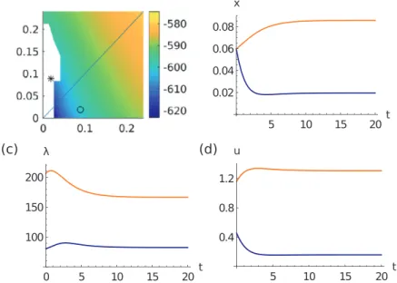
Problem(1a)–(1c) hasauniqueCSSX_∞,withA(^X∞)=R+,cf.Fig.1(a).Moreover,Fig.1(b)showsthetime–dependent CP X(^t)≡(^x(^t),

λ

(^t))^startingatx0=0.03,andthepath oftheassociatedoptimalcontrol u^∗(^t)^{.Here, theinitialstockis} lowerthanitssteadystate;thatis,x₀=0.03<0.0596=x_∞.Thisimpliesthatatthebeginningoftheperiod,theagenthas tospendaratherhighcultivationefforttoincrease thestock, whilethiseffortmaybereducedasthestockincreasesover time.Likewise,theshadowpriceofthestockisinitiallyquitehighbutmonotonouslydecreasesasthestockbecomesmore abundant.

3. Stock–enhancementinatwo-patchmodel

Letusnowconsiderasystemoftwodiffusivelycoupledpatcheswithstocksx1andx2thatdispersebetweenthepatches withconstant per-capitadispersal rateD.(Thinkoftwopenguin coloniesattwo distinctlocations, whereindividual pen- guinscanmigratefromonepatchtoanother,andnetmigrationistowardsthelocationoflowbiomassconcentration.)The populationdynamicsofthetwopatchesareidentical(i.e.,theyhavethesamecarryingcapacityKandexogenouslossrate

δ

⁾

andcanbecontrolledinthesamewaybypatch-specificstock-enhancementactivities u₁andu₂.Assumingthatthestocks areagainmeasuredinunitsofthecarryingcapacity,thestateequation(1a)generalisesto(suppressingthetimeargument)

x˙i= fi

(

^x,ui

)

≡uixi

(

¹−xi

)

−

δ

^xi+D

(

^x3−i−xi

)

, i=1,2 (6a) withx≡(^x1,x₂)^.Lettingu≡(^u1,u₂),astraightforwardextensionof(1b)yieldstheinstantaneousutility

Jc

(

^x,u

)

≡ 2

i=1

Jc,i

(

^xi,ui

)

, with Jc,i

(

^xi,ui

)

≡log

(

^xi

)

−

γ

2u²_i. Theproblemoftheagentis

max

u∈U² J

(

^x

(

^·

)

^,u

(

^·

))

^{, where J}

(

^x

(

^·

)

^,u

(

^·

))

^{≡ ∞}

0

e^−ρtJc

(

^x

(

^t

)

^,u

(

^t

) )

^{dt, (6b)}

subjecttothestockdynamics(6a).Then,theHamiltonianreadsas H

(

^x,u,

λ )

^≡Jc

(

^x,u

)

⁺

λ

^·f

(

^x,u

)

^,

with the costate vector

λ

≡(

λ

1,

λ

2), stockdynamics f≡(^f1,f₂), and the limiting intertemporal transversality condition lim_t→∞e^−ρtx(^t)·

λ

(^t)=0,where again we can apply Tauchnitz (2015), cf.Appendix B. Maximising H withrespect to u yields the optimal controls u^∗_i = ^λ_γⁱx_i(¹−x_i)^{. As expected, we obtain the same rule for the optimal} stock–enhancement policy asin theone-patchcase. However, thisdoesnot rule out(as we shallsee) that we mayfindsolutions that differ fromtheoptimalcontrolintheone-patchcase.

Now,bysubstitutingtheoptimalcontrolsintothestateequations(6a)andthecostateequations

λ

˙i=

ρλ

i−

∂

^H/

∂

^xi,we obtainthecanonicalsystem

˙

xi

(

^t

)

=

λ

i

γ

^x2i

⁽

^1−xi

⁾

²⁻

δ

^xi+D

(

^x3−i−xi

)

^{, (7a)}

6In a 2-component ODE (scalar state ODE), this can be done by (essentially) integrating backward in time from the stable eigenspace but in higher dimensions—for example, in case of two patches (see Section 3 ), or in case of high dimensional ODEs obtained from spatial discretizations of PDEs (see Sections 4 and 5 )—such computations of stable manifolds become infeasible. See Grass et al. (2008) and Uecker (2016) for comments on the nu- merical method for computing canonical paths by truncation to large T and suitable asymptotic boundary conditions, and how this relates to the saddle point property of CSSs.

Table 1

Properties of the CSSs of system (7) with parameter values (8) . The system exhibits a flat CSS X _∞^f and a pair of POSSs, X _∞^p and X ^p_∞, which are identical up to the exchange of patch indices.

CSS x 1,2 λ1,2 u ^∗_1,2 J SPP Remarks

0.0596 189.61 1.063 not optimal, dominated by the path to X ^p∞with value J CP = −602 . 6

Flat: X ∞^f -677.9 no

0.0596 189.61 1.063

0.086 166.37 1.305 optimal, hence a POSS and “almost” globally stable

Patterned: X ^p_∞, X ^p_∞ -601.1 yes

0.0196 82.5 0.158

Fig. 1. Optimal solution of the non-spatial stock-enhancement system. (a) Phase portrait of the canonical system (5) , showing the saddle point X ∞(black point), and its stable (green) and unstable manifold (orange). Selected orbits are shown in blue. The vertical-dashed line marks the initial stock value x 0= 0 . 03 . In the optimal orbit, the initial costate λ0is chosen to be located exactly on the intersection of that line with the stable manifold of X ∞, yielding λ0= 412 . 64 (grey point). (b) Time dependence of the optimal orbit (x, λ) and of the optimal control u ^∗for the initial value x 0= 0 . 03 . The canonical path corresponds to the part of the stable manifold between the grey and the black point. (For the visibility of the colouring the reader is referred to the web version of this article.)

λ

˙i

(

^t

)

=

λ

i

( δ

⁺

ρ )

⁻

λ

²ix_i

(

^1−2xi

) (

^1−xi

)

γ

⁻

1

x_i−D

( λ

3−i−

λ

i

)

^{, (7b)}

withinitialvaluesx_i(⁰)=x_i,0.Remarkably,whilethespatialcouplinginthestateequation(7a)isdescribedbythe‘diffusion’

term D(^x3−i−x_i), thecoupling inthe costateequation (7b)is describedby the‘anti-diffusion’ term−D(

λ

3−i−

λ

i)^.Thus, whilethediffusion-drivenresourceflowisfromhightowardslowconcentrations(i.e.,fromthecrowdedtothelesscrowded area),anoptimalstock–enhancingpolicymakestheshadowpriceoftheresource‘move’fromlowtohighprices.

Irrespectiveofthevalue ofthedispersalrateD≥0,thecanonicalsystem(7)hasthehomogeneous (orflat) CSS:X_∞^f = (^x∞,x_∞,

λ

∞,

λ

∞)^{(i.e.,twice the CSSX}∞ ofthe singlepatch modelofSection 2).By settingD=0.25 andusingthesame parametervaluesasintheprevioussection:

D=0.25,

ρ

^=0.025,

γ

^=10,

δ

^{=1, (8)}

weobtainx_1∞=x_2∞=0.0596,

λ

1∞=

λ

2∞=189.61,andu^∗_1∞=u^∗_2∞=1.0634,whichexactlyreplicatesthevaluesfromthe non-spatialmodel.Correspondingly,theinstantaneousbenefitandthetotalprofitforthissolutionaresimplydoubledcom- pared tothe non-spatialmodel: J_c(^X∞^f )=2J_c(^X∞)=−16.95andJ(^X∞^f )=2J(^X∞)=−677.9.In addition,we find a hetero- geneous (or patterned) CSS X_∞^p =(^x1,x₂,

λ

1,

λ

2) ^fori=1,2,where the valuesofthe stocks, x₁=0.086, x₂=0.0196,the costates,

λ

1=166.37,

λ

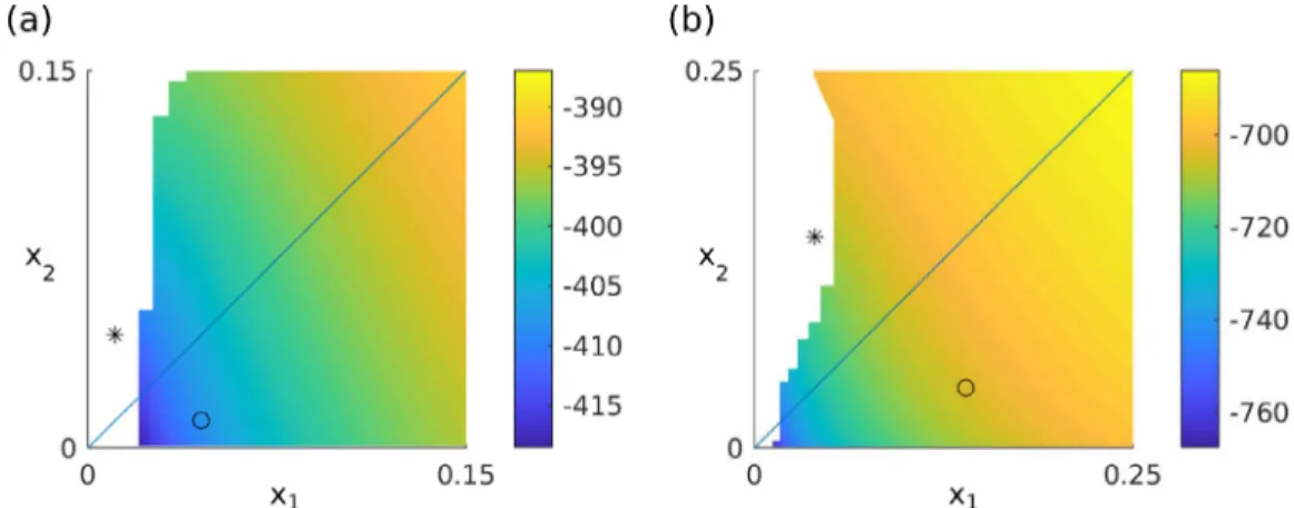
2=82.505,andtheoptimalcontrols,u^∗₁=1.305,u^∗₂=0.158,differinthetwopatches.The result- ing instantaneousbenefitisJc(^X∞^p)=−15.03,thediscountedprofitisJ(^X∞^p)=−601.1,andhencethepatternedCSSyields

Fig. 2. (a) Domain of attraction A (X ^p∞), and values of the CP from X (0)∈ R ²₊to X ^p∞, marked by ◦for the two patch model with parameter values (8) . Initial states for which no CP to X ^p_∞could be found are left white. The mirrored X ^p_∞is marked by ∗, and A (X _∞^p) and the values of CPs are naturally obtained by mirroring the plot at the diagonal. (b)–(d) CP from the stock of X _∞^f to X _∞^p; time dependence of the state variables, the costates and the optimal controls for both patches.

ahigherutilitycomparedtotheflatCSS.Naturally,by exchangingthetwopatches,wefindasecondequivalentpatterned CSSX_∞^p =(^x2,x₁,

λ

2,

λ

1)^.7

HavingfoundthesethreeCSSs,thenext questionreferstotheirstabilityanddomainsofattraction.Thatis,givensome initial state x₀, whichofthesethree canbe reachedbya CPfromx(⁰)=x₀,andifwe canreach morethanone, which of the CPs yields the highest profit. A simple visualization such as the phase plane plotin Fig. 1 is no longer possible because thecanonical systemofthetwo-patch modelis4–dimensional.Locally, a CSSX_∞ ofa 2n–dimensionalcanonical systemhasthesaddlepointproperty(SPP)ifthedimensionofitsstablemanifolddimWs(^X∞)^equalsn;correspondingly,the numberd≡n−dimW_s(^X∞)^{iscalledthedefectoftheCSS(seeGrassetal.,2008),andthesenumberscanbecomputedby} linearizationof(6a)aroundX_∞.Thedimensionofthestablemanifold,dimWs(^X∞),equalsthenumberofeigenvaluesofthe linearizationwithnegativerealparts.

Forourchosen parameter values,onlythepatterned CSSX_∞^p (and naturallyalsoX_∞^p) hastheSPP. Incontrast,the flat CSSX_∞^f doesnothavetheSPP:the dimensionofits stablemanifoldequals dimWs(^X∞^f )=ns=1, andthus itsdefectd= 2−1>0.Consequently,canonicalpathstotheflatCSSX_∞^f onlyexistforparticularvaluesofx₀onaone-dimensionalcurve;

namely,thoseforwhichthereexistsa

λ

(⁰)^suchthat(^x(⁰),

λ

(⁰))^{islocatedinthestablemanifoldofX}∞^f.Suchadefective CSS(i.e.,whend>0)maystillbeoptimalifacanonicalpathtoanotherCSSdoesnotexist.

Meanwhile, thepatternedCSSX^p_∞ is“almostgloballystablemodulosymmetry”.Bythiswemeanthat forallx₀∈R²₊, possiblyexceptforasmallsetnear(0,0)(seebelow),initialcostates

λ

(⁰)^{canbefoundsuchthatacanonicalpathtoX}∞^p or X_∞^p (orboth)exist.InFig.2(a),weshowthevaluesoftheCPsfromsomearbitraryinitialpointx₀toX_∞^p,withthex–values ofX_∞^p markedbya◦,andthewhitepartindicatingthesetofinitialstatesforwhichaCPtoX_∞^p couldnotbefound.This includes,forinstance,X_∞^p,indicated bythe∗.However, A(^X∞^p)^{containsatleastthecolouredset,andnaturally}A(^X∞^p)^is obtainedfrommirroringalongthediagonal,suchthatbysymmetrythediagonalisaSkibamanifoldbetweenX^p_∞andX_∞^p. Forx0∈A(^X∞^p)∩A(^X∞^p),thisSkibamanifoldyieldsthe(expected)resultthatbelowthediagonalitisoptimaltogotoX_∞^p, andabovethediagonaltoX_∞^p.Together,A(^Xp∞)∪A(^X∞^p) ^coverR²₊,exceptfora smallsetnearx=0,butwebelieve that thisisduetoournumericalmethod.Wediscretizethepositivequadrantbyagrid(^x1,x₂)i j andforeachinitialstateofthat gridaimtocomputetheCPtoX_∞^p withafixedmethod,such aswitha fixedtruncationtime T.Thisleavesopen aregion near(^x1,x₂)=(⁰,0)^{(whereasinFig.1theinitialco–statesgoto}∞),butbytweakingthenumerics(e.g.,usingafinergrid ofinitialstates,andadaptingT),wecanshrinkthenon-existenceregionnear(^x1,x₂)=(⁰,0)^.

Supposethatinthepastthetwo patcheshavebeenmanagedbytwodifferentagents(orfirms),butthatanintegrated managementofbothpatcheswillbeconsideredfromnowon.Then,thequestionishowcanwebestgoverntheintegrated systemofthe twopatches totheoptimal(which heremeans tothepatterned,steadystate)? However, thisis aquestion aboutthebestpolicyduringthetransitiontimefromtheflatCSStothepatternedCSS—oraboutthecanonicalpath.Fig.2(b)

7The CSSs and the CPs discussed were subsequently found using the toolbox pde2pathby first treating (7) as a bifurcation problem for steady states and then computing the CPs by a truncated continuation problem in the initial states, but we postpone these bifurcation and computation issues to the next Section.

displaysthe CPfromthe initial stockx₀=x_∞^f =(^x∞,x_∞)^{of theflat CSS(on thediagonal) to thepatterned CSSX}∞^p. The discountedprofitofthisCPisJ_CP=−602.6,whichishigherthanthediscountedprofitJ(^X∞^f )=−677.9ofthestartingCSS.

Thus, we mayin fact characterizethe patterned CSS X_∞^p asa patterned optimalsteady state (POSS),unique modulo the symmetryofinterchangingpatch1and2.

Thesecomputationsarebasedontheassumptionofaperfectlyhomogeneoussystem.Thissymmetryis,ofcourse,broken ifanyofthemodelparameters dependsonthepatchi,such asby assumingdifferentexogenouslossrates

δ

1=

δ

2.Ifthe symmetrybreakingisweak(i.e.,

δ

1≈

δ

2)thentheflatCSSsurvivesasan‘almostflat’CSS,andthetwoequivalentpatterned CSS X_∞^p andX_∞^p become two differentpatterned CSS.⁸ Itthen becomesan interesting taskto characterizetheir domains of attractions,which are alsono longerrelatedby simple symmetry. However, ourpoint hereisto deliberately focuson the symmetric(i.e.,spatially homogeneous)case.Ourresultsshow thateven thoughthemodel isspatiallyhomogeneous, positive dispersal ratesmaygive riseto aspatially non-homogeneous(orpatterned) optimalsolution.Thisresultisquite surprising,becausedispersal,withmovementfromthecrowdedtothelesscrowdedpatch, persetendstoflattenout the stockoverthespatialdomain.Thus,arathersimplestock–enhancementmodelwithtwopatchesmaybringaboutcounter- intuitive optimalpolicies.Thenatural,thoughtentative,policyproposalcallingforanequaldistributionoftheefforts(and thusofthecost)maybemisled.

4. Stock–enhancementinaone-dimensionalcontinuousspace

We nowextendourmodelto acontinuousone–dimensional(1D)space, andassumethat theresourceiscontinuously distributedoveraboundedinterval⊂R.Theagentmaythenchoosethestock–enhancingactivityatanyspatiallocation z∈^{; that is,the agentcan select(at each instant oftime) afunction u}(·,t) ^on , rather thana scalar u(^t),asin the non-spatialmodel,ora2D vectoru(^t),asinthetwo-patchmodel.Accordingly,we generalisethestockdynamics(6a) to thereaction–diffusionequation

∂

^tx

(

z,t

)

=u

(

z,t

)

^x

(

z,t

)(

¹−x

(

z,t

))

−

δ

^x

(

z,t

)

+D x

(

z,t

)

^(9a)

with diffusionconstant D andinitial condition(initialdistribution) x(^z,0)=x₀(^z),

∀

^z∈^{.9 In (9a),we followFick’s first} lawofdiffusion,postulatingthatthefluxofthebiomassgoesfromregionsofhightothoseoflowconcentration,wherethe magnitudeofthefluxisproportionaltotheconcentrationgradient(spatialderivative).Moreover,weassumehomogeneous Neumannboundaryconditions(BCs),modellingtheideathatthestockcanliveat,butcannottraversetheboundaryofthe habitat,andthusimplyingtheabsenceofanyexteriorin-oroutflow(seeAppendixAforgeneralizationtoRobinBCs):

∂

nx

(

z,t

)

=0,

∀

^z∈

∂

, (9b)

where

∂

^{nistheoutwardnormalderivative(the derivativetakeninthedirectionorthogonaltotheboundaryof).In1D,} wherethespatialdomainisaninterval,=(^a,b),wehave,suppressingthetimeargument,

∂

nx(^a)=−x(^a)^and

∂

nx(^b)= x(^b),and x(^z)=x(^z)^{(seealsofn.9).}

Assumingagainthattheinstantaneouspointwiseutilityisgivenby (1b)—thatis,Jc(^x,u)≡log(^x)−^γ₂u²—,we writethe spatialaverageofJ_cover^as

Jca

(

^t

)

≡ 1

| |

Jc

(

^x

(

z,t

)

,u

(

z,t

) )

^dz,

andtheagentseekstomaximizethediscountedaverageutility

maxu∈U J

(

^x

(

^·

)

^,u

(

^·

))

^{where J}

(

^x,u

)

^≡∞

0

e^−ρtJca

(

^x,u

)

^{dt (9c)}

subjectto(9a)and(9b),andwiththeoptimalcontrolasgivenin(4).TheformalHamiltonianforproblem(9)isthengiven by

H≡Jca

(

^t

)

⁺

|

¹

|

λ (

^z,t

)

^f

(

^x

(

^z,t

)

^,u

(

^z,t

))

^{dz, (10)}

where f(^x,u)≡h(^x,u)+D xdenotestheright-handsideof(9a).

To derive thecanonical systemfor problem(9),we need to take thevariational derivative ofH withrespect to x. To do so,we use integrationby parts ofthe term

λ

^{x occurringinH},and apply Pontryagin’smaximum principle (see the Appendixforfurthercomments)withthelimitingintertemporaltransversalitycondition

tlim→∞e^−ρt

λ (

z,t

)

^x

(

z,t

)

^dz=0. (11)

8In the Appendix, we illustrate this for the spatially continuous model by breaking symmetry via boundary conditions.

9The Laplace operator ≡∇·∇≡∇²denotes the divergence of the gradient of a function fon Euclidean space. In Cartesian coordinates, it is the sum of second partial derivatives of fwith respect to the independent variables, which here consist of the spatial coordinates: f(^z)= ⁿi=1∂z²if(^z).