Boolean Functions for Cryptography and Error Correcting Codes

(1)

Boolean Functions for Cryptography and Error Correcting Codes

Claude Carlet^∗

∗LAGA, University of Paris 8, France; e-mail: claude.carlet@univ-paris8.fr.

(2)

1 Introduction

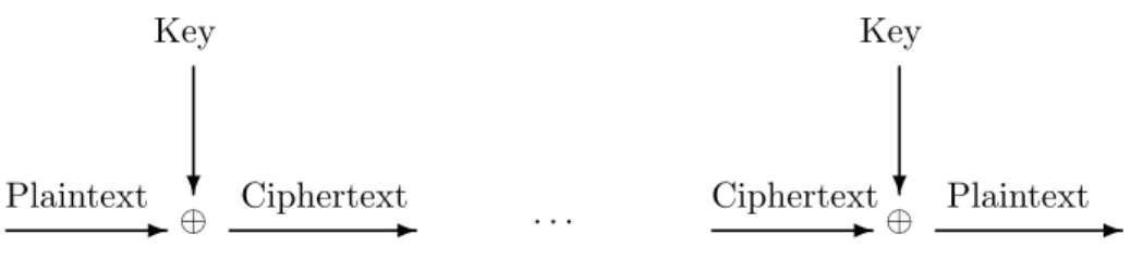
A fundamental objective ofcryptography is to enable two persons to communicate over an insecure channel (a public channel such as internet) in such a way that any other person is unable to recover their message (called the plaintext) from what is sent in its place over the channel (the ciphertext).

The transformation of the plaintext into the ciphertext is calledencryption, or enciphering. Encryption-decryption is the most ancient cryptographic activity (ciphers already existed four centuries B. C.) but its nature has deeply changed with the invention of computers, because the cryptanalysis (the activity of the third person, the eavesdropper, who aims at recovering the message) can use their power.

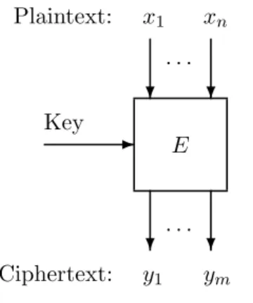
The encryption algorithm takes as input the plaintext and an encryption keyKE, and it outputs the ciphertext. If the encryption key is secret, then we speak of conventional cryptography, of private key cryptography or of symmetric cryptography. In practice, the principle of conventional cryptography relies on the sharing of a private key between the sender of a message (often called Alice in cryptography) and its receiver (often called Bob). If, on the contrary, the encryption key is public, then we speak of public key cryptography. Public key cryptography appeared in the literature in the late seventies.

Thedecryption (or deciphering) algorithm takes as input the ciphertext and a secret¹ decryption key KD. It outputs the plaintext.

- Decryption

- Encryption -

plaintext ciphertext plaintext

public channel

K_E K_D

b b

Public key cryptography is preferable to conventional cryptography, since it allows to securely communicate without having previously shared keys in a secure way: every person who wants to receive secret messages can keep secret a decryption key and publish an encryption key; ifnpersons want to secretly communicate pairwise using a public key cryptosystem, they needn

1According to principles already stated in 1883 by A. Kerckhoffs [212], who cited a still more ancient manuscript by R. du Carlet [50], only the secret keys must be kept secret – the confidentiality should not rely on the secrecy of the encryption method – and a cipher cannot be considered secure if it can be decrypted by the designer himself.

(6)

encryption keys and n decryption keys, when conventional cryptosystems will need ⁿ₂

= ⁿ⁽ⁿ⁻¹⁾₂ keys. But all known public key cryptosystems are much less efficient than conventional cryptosystems (they allow a much lower data throughput) and they also need much longer keys to ensure the same level of security. This is why conventional cryptography is still widely used and studied nowadays. Thanks to public key cryptosystems, the share-out of the necessary secret keys can be done without using a secure channel (the secret keys for conventional cryptosystems are strings of a few hundreds of bits only and can then be encrypted by public key cryptosystems). Proto- cols specially devoted to key-exchange can also be used.

The objective oferror correcting codesis to enable digital communication over a noisy channel in such a way that the errors in the transmission of bits can be detected²and corrected by the receiver. This aim is achieved by using an encoding algorithm which transforms the information before sending it over the channel. In the case of block coding³, the original message is treated as a list of binary words (vectors) of the same length – say k – which are encoded into codewords of a larger length – say n. Thanks to this extension of the length, calledredundancy, the decoding algorithm can correct the errors of transmission (if their number is, for each sent word, smaller than or equal to the so-called correction capacity of the code) and recover the correct message. The set of all possible codewords is called the code. Sending words of length n over the channel instead of words of lengthk slows down the transmission of information in the ratio of ^k_n. This ratio, called thetransmission rate, must be as high as possible, to allow fast communication.

-Decoding

-Encoding -

message codeword message

noisy channel

In both cryptographic and error correcting coding activities, Boolean functions (that is, functions from the vectorspaceFⁿ₂ of all binary vectors of

2If the code is used only to detect errors, then when an error is detected, the information must be requested and sent again in a so-called “automatic request” procedure.

3We shall not address convolutional coding here.

(7)

lengthn, to the finite field with two elements⁴ F2) play roles:

- every code of length 2ⁿ, for some positive integer n, can be interpreted as a set of Boolean functions, since every n-variable Boolean function can be represented by its truth table (an ordering of the set of binary vectors of length n being first chosen) and thus associated with a binary word of length 2ⁿ, and vice versa; important codes (Reed-Muller, Kerdock codes) can be defined this way as sets of Boolean functions;

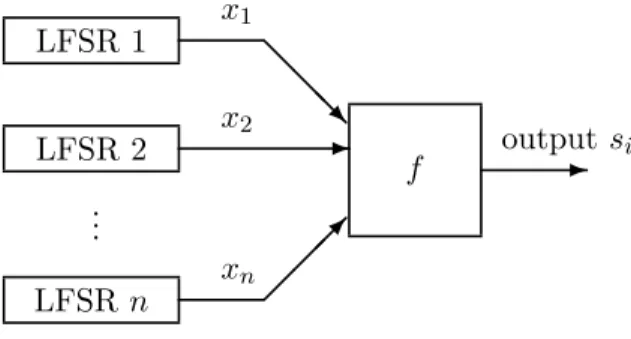
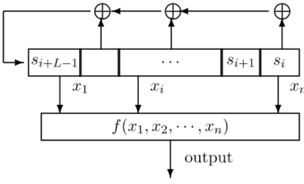
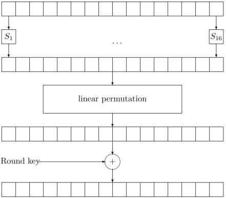
- the role of Boolean functions in conventional cryptography is even more important: cryptographic transformations (pseudo-random generators in stream ciphers, S-boxes in block ciphers) can be designed by appropriate composition of nonlinear Boolean functions.

In both frameworks, n is rarely large, in practice. The error correcting codes derived from n-variable Boolean functions have length 2ⁿ; so, tak- ingn= 10 already gives codes of length 1024. For reason of efficiency, the S-boxes used in most block ciphers are concatenations of sub S-boxes on at most 8 variables. In the case of stream ciphers, n was in general at most equal to 10 until recently. This has changed with the algebraic attacks (see [113, 117, 150] and see below) but the number of variables is now most often limited to 20.

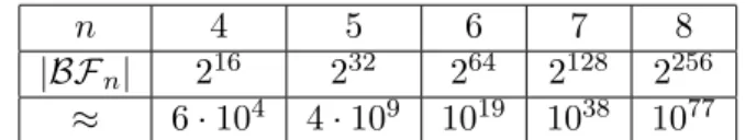
Despite the fact that Boolean functions are currently used in cryptography and coding with low numbers of variables, determining and studying those Boolean functions satisfying the desired conditions (see Subection 4.1 below) is not feasible through an exhaustive computer investigation: the number|BF_n|= 2²ⁿ ofn-variable Boolean functions is too large whenn≥6.

We give in table 1 below the values of this number fornranging between 4 and 8.

n 4 5 6 7 8

|BF_n| 2¹⁶ 2³² 2⁶⁴ 2¹²⁸ 2²⁵⁶

≈ 6·10⁴ 4·10⁹ 10¹⁹ 10³⁸ 10⁷⁷

Table 1: Number of n-variable Boolean functions

Assume that visiting ann-variable Boolean function, and determining whe- ther it has the desired properties, needs one nano-second (10⁻⁹ seconds), then it would need millions of hours to visit all functions in 6 variables, and about one hundred billions times the age of the universe to visit all those in 7 variables. The number of 8-variable Boolean functions approximately equals the number of atoms in the whole universe! We see that trying to find

4Denoted byBis some chapters of the present collection.

(8)

functions satisfying the desired conditions by simply picking up functions at random is also impossible for these values of n, since visiting a non- negligible part of all Boolean functions in 7 or more variables is not feasible, even when parallelizing. The study of Boolean functions for constructing or studying codes or ciphers is essentially mathematical. But clever computer investigation is very useful to imagine or to test conjectures, and sometimes to generate interesting functions.

2 Generalities on Boolean functions

In this chapter and in the chapter “Vectorial Boolean Functions for Cryp- tography” which follows, the set{0,1}will be most often endowed with the structure of field (and denoted byF2), and the setFⁿ₂ of all binary vectors⁵ of lengthnwill be viewed as anF2-vectorspace. We shall denote simply by 0 the null vector in Fⁿ₂. The vectorspace Fⁿ₂ will sometimes be also endowed with the structure of field – the fieldF2ⁿ (also denoted by GF(2ⁿ)); indeed, this field being an n-dimensional vectorspace over F2, each of its elements can be identified with the binary vector of lengthnof its coordinates relative to a fixed basis. The set of all Boolean functionsf :Fⁿ₂ →F2 will be denoted as usual by BF_n. The Hamming weight wH(x) of a binary vector x ∈ Fⁿ₂ being the number of its nonzero coordinates (i.e. the size of{i∈N/ x_i 6= 0}

where N denotes the set {1,· · ·, n}, called the support of the codeword), the Hamming weight wH(f) of a Boolean function f on Fⁿ₂ is (also) the size of the support of the function , i.e. the set {x ∈Fⁿ2/ f(x) 6= 0}. The Hamming distance d_H(f, g) between two functionsf andg is the size of the set{x∈Fⁿ₂/ f(x)6=g(x)}. Thus it equals wH(f⊕g).

Note. Some additions of bits will be considered in Z (in characteristic 0) and denoted then by +, and some will be computed modulo 2 and denoted by ⊕. These two different notations will be necessary because some representations of Boolean functions will live in characteristic 2 and some representations of the same functions will live in characteristic 0. But the additions of elements of the finite field F2ⁿ will be denoted by +, as it is usual in mathematics. So, for simplicity (since Fⁿ2 will often be identified withF2ⁿ) and because there will be no ambiguity, we shall also denote by + the addition of vectors ofFⁿ₂ when n >1.

5Coders say “words”

(9)

2.1 Representation of Boolean functions

Among the classical representations of Boolean functions, the one which is most usually used in cryptography and coding is then-variable polynomial representation overF2, of the form

f(x) = M

I∈P(N)

aI

Y

i∈I

xi

!

= M

I∈P(N)

aIx^I, (1) whereP(N) denotes the power set of N ={1,· · ·, n}. Every coordinate x_i appears in this polynomial with exponents at most 1, because every bit inF2

equals its own square. This representation belongs to F2[x1,· · ·, xn]/(x²₁⊕ x₁,· · ·, x²_n⊕x_n). It is called theAlgebraic Normal Form (in brief the ANF).

Example: let us consider the functionf whose truth-table is x1 x2 x3 f(x)

0 0 0 0

0 0 1 1

0 1 0 0

0 1 1 0

1 0 0 0

1 0 1 1

1 1 0 0

1 1 1 1

It is the sum (modulo 2 or not, no matter) of the atomic functions f1, f2

and f₃ whose truth-tables are

x1 x2 x3 f1(x) f2(x) f3(x)

0 0 0 0 0 0

0 0 1 1 0 0

0 1 0 0 0 0

0 1 1 0 0 0

1 0 0 0 0 0

1 0 1 0 1 0

1 1 0 0 0 0

1 1 1 0 0 1

The functionf₁(x) takes value 1 if and only if 1⊕x₁ = 1, 1⊕x₂ = 1 and x₃ = 1, that is if and only if (1⊕x₁)(1⊕x₂)x₃ = 1. Thus the ANF of f₁

(10)

can be obtained by expanding the product (1⊕x1)(1⊕x2)x3. After similar observations on f₂ and f₃, we see that the ANF of f equals (1⊕x₁)(1⊕ x₂)x₃⊕x₁(1⊕x₂)x₃⊕x₁x₂x₃ =x₁x₂x₃⊕x₂x₃⊕x₃. 2 Another possible representation of this same ANF uses an indexation by means of vectors of Fⁿ₂ instead of subsets of N; if, for any such vector u, we denote byau what is denoted by a_supp(u) in Relation (1) (wheresupp(u) denotes the support ofu), we have the equivalent representation:

f(x) = M

u∈Fⁿ₂

a_u





n

Y

j=1

x_j^u^j



.

The monomialQn

j=1xjuj is often denoted byx^u.

Existence and uniqueness of the ANF By applying the Lagrange in- terpolation method described in the example above, it is a simple matter to show the existence of the ANF of every Boolean function. This implies that the mapping, from every polynomialP ∈F2[x₁,· · ·, x_n]/(x²₁⊕x₁,· · ·, x²_n⊕ x_n) to the corresponding function x ∈ Fⁿ₂ 7→ P(x), is onto BF_n. Since the size ofBF_n equals the size ofF2[x1,· · ·, xn]/(x²₁⊕x1,· · ·, x²_n⊕xn), this correspondence is one to one⁶. But more can be said.

Relationship between a Boolean function and its ANF The product x^I = Q

i∈Ixi is nonzero if and only if xi is nonzero (i.e. equals 1) for everyi∈I, that is, if I is included in the support of x; hence, the Boolean functionf(x) =L

I∈P(N)a_Ix^I takes value f(x) = M

I⊆supp(x)

aI, (2)

where supp(x) denotes the support of x. If we use the notation f(x) = L

u∈Fⁿ₂ a_ux^u, we obtain the relation f(x) = L

uxa_u, where u x means that supp(u) ⊆ supp(x) (we say that u is covered by x). A Boolean functionf^◦ can be associated to the ANF of f: for everyx∈Fⁿ₂, we setf^◦(x) = a_supp(x), that is, with the notation f(x) = L

u∈Fⁿ₂ a_ux^u: f^◦(u) = a_u. Re- lation (2) shows that f is the image of f^◦ by the so-called binary M¨obius

6Another argument is that this mapping is a linear mapping from a vectorspace overF2

of dimension 2ⁿto a vectorspace of the same dimension.

(11)

transform.

The converse is also true:

Proposition 1 Let f be a Boolean function on Fⁿ₂ and let L

I∈P(N)aIx^I be its ANF. We have:

∀I ∈ P(N), a_I = M

x∈Fⁿ₂/ supp(x)⊆I

f(x). (3)

Proof. Let us denote L

x∈Fⁿ₂/ supp(x)⊆If(x) by b_I and consider the func- tiong(x) =L

I∈P(N)bIx^I. We have g(x) = M

I⊆supp(x)

bI = M

I⊆supp(x)





M

y∈Fⁿ2/ supp(y)⊆I

f(y)





and thus

g(x) = M

y∈Fⁿ2

f(y)





M

I∈P(N)/ supp(y)⊆I⊆supp(x)

1



. The sum L

I∈P(N)/ supp(y)⊆I⊆supp(x)1 is null if y 6= x, since the set {I ∈ P(N)/ supp(y)⊆I ⊆supp(x)}contains 2^w^H^(x)−w^H^(y)elements ifsupp(y)⊆ supp(x), and none otherwise. Hence,g=f and, by uniqueness of the ANF,

b_I=a_I for everyI. 2

Algorithm There exists a simple divide-and-conquer butterfly algorithm to compute the ANF from the truth-table (orvice-versa), that we can call the Fast M¨obius Transform. For every u= (u1,· · ·, un)∈Fⁿ2, the coefficient au

ofx^u in the ANF of f equals M

(x1,···,xn−1)(u1,···,un−1)

[f(x1,· · ·, xn−1,0)] ifun= 0 and M

(x1,···,xn−1)(u₁,···,un−1)

[f(x₁,· · ·, xn−1,0)⊕f(x₁,· · ·, xn−1,1)] if u_n= 1.

Hence if, in the truth-table of f, the binary vectors are ordered in lexicographic order, with the bit of higher weight on the right, the table of the ANF equals the concatenation of the ANFs of the (n−1)-variable functions f(x1,· · ·, xn−1,0) andf(x1,· · ·, xn−1,0)⊕f(x₁,· · ·, xn−1,1). We deduce the following algorithm:

(12)

1. write the truth-table off, in which the binary vectors of length nare in lexicographic order as decribed above;

2. let f0 and f1 be the restrictions of f to Fⁿ⁻¹₂ × {0} and Fⁿ⁻¹₂ × {1}, respectively⁷; replace the values of f₁ by those off₀⊕f₁;

3. apply recursively step 2, separately to the functions now obtained in the places off₀ and f₁.

When the algorithm ends (i.e. when it arrives to functions in one variable each), the global table gives the values of the ANF off. The complexity of this algorithm is ofn2ⁿ XORs.

Remark.

The algorithm works the same if the vectors are ordered in standard lexicographic order, with the bit of higher weight on the left (indeed, this corresponds to applying it tof(xn, xn−1,· · ·, x1)).

The degree of the ANF is denoted by d^◦f and is called the algebraic degree of the function (this makes sense thanks to the existence and uniqueness of the ANF):d^◦f = max{|I|/ a_I 6= 0}, where |I|denotes the size of I.

Some authors also call it the nonlinear order off. According to Relation (3), we have:

Proposition 2 The algebraic degreed^◦f of anyn-variable Boolean function f equals the maximum dimension of the subspaces {x ∈ Fⁿ2/ supp(x) ⊆ I}

on whichf takes value 1 an odd number of times.

The algebraic degree is anaffine invariant (it is invariant under the action of the general affine group): for every affine isomorphism L :





 x₁ x2

... xn







∈

Fⁿ2 7→M×





 x₁ x2

... xn







⊕





 a₁ a2

... an







∈Fⁿ2 (where M is a nonsingular n×nmatrix

7The truth-table of f0 (resp. f1) corresponds to the upper (resp. lower) half of the table off.

(13)

over F2), we have d^◦(f ◦L) = d^◦f. Indeed, the composition by L clearly cannot increase the algebraic degree, since the coordinates ofL(x) have degree 1. Hence we have d^◦(f ◦L) ≤ d^◦f (this inequality is more generally valid for every affine homomorphism). And applying this inequality tof◦L in the place off and toL⁻¹ in the place of Lshows the inverse inequality.

Two functionsf and f◦L whereL is anF2-linear automorphism of Fⁿ₂ (in the case casea1 =a2=· · ·=an= 0 above) will be calledlinearly equivalent and two functions f and f ◦L, where L is an affine automorphism of Fⁿ2, will be calledaffinely equivalent.

The algebraic degree being an affine invariant, Proposition 2 implies that it also equals the maximum dimension of all the affine subspaces of Fⁿ2 on which f takes value 1 an odd number of times.

It is shown in [297] that, for every nonzeron-variable Boolean function f, denoting by g the binary M¨obius transform of f, we have d^◦f +d^◦g ≥ n.

This same paper deduces characterizations and constructions of the functions which are equal to their binary M¨obius transform, called coincident functions.

Remarks.

1. Every atomic function has algebraic degreen, since its ANF equals (x1⊕ ₁)(x₂⊕₂)· · ·(x_n⊕_n), where _i ∈ F2. Thus, a Boolean function f has algebraic degree n if and only if, in its decomposition as a sum of atomic functions, the number of these atomic functions is odd, that is, if and only ifw_H(f) is odd. This property will have an important consequence on the Reed-Muller codes and it will be also useful in Section 3.

2. If we know that the algebraic degree of an n-variable Boolean functionf is bounded above byd < n, then the whole function can be recovered from some of its restrictions (i.e., a unique function corresponds to this partially defined Boolean function). Precisely, according to the existence and uniqueness of the ANF, the knowledge of the restriction f_|E of the Boolean function f (of algebraic degree at most d) to a set E implies the knowledge of the whole function if and only if the system of the equations f(x) = L

I∈P(N)/|I|≤da_Ix^I, with indeterminates a_I ∈ F2, and where x ranges over E (this makes |E| equations), has a unique solution⁸. This happens with the setE_d of all words of Hamming weights smaller than or equal tod, since Relation (3) gives the value ofaI (whenI ∈ P(N) has size

8Takingf|E null leads to determining the so-called annihilators of theindicator ofE (the function 1E, also called characteristic function ofE, defined by 1E(x) = 1 if x∈E and 1E(x) = 0 otherwise); this is the core analysis of Boolean functions from the viewpoint of algebraic attacks, see Subsection 4.1.

(14)

|I| ≤d). Notice that Relation (2) allows then to express the value of f(x) for everyx∈Fⁿ₂ by means of the values taken byf at all words of Hamming weights smaller than or equal tod. We have (using the notation a_u instead ofaI, see above):

f(x) = M

ux

a_u = M

ux u∈Ed

a_u= M

yx y∈Ed

f(y)|{u∈E_d/ yux|

= M

yx y∈Ed

f(y)









d−w_H(y)

X

i=0

wH(x)−wH(y) i



 [mod 2]



.

More generally, the whole function f can be recovered from f|E for every set E affinely equivalent to E_d, according to the affine invariance of the algebraic degree. This also generalizes to “pseudo-Boolean” (that is, real- valued) functions, if we consider the numerical degree (see below) instead of

the the algebraic degree,cf. [350]. 2

The simplest functions, from the viewpoint of the ANF, are those Boolean functions of algebraic degrees at most 1, calledaffine functions:

f(x) =a₁x₁⊕ · · · ⊕a_nx_n⊕a₀.

They are the sums of linear and constant functions. Denoting bya·x the usual inner product a·x = a1x1⊕ · · · ⊕anxn in Fⁿ₂, or any other inner product (symmetric and such that, for everya6= 0, the function x →a·x is a nonzero linear form on Fⁿ₂), the general form of an n-variable affine function isa·x⊕a0 (with a∈Fⁿ₂; a0 ∈F2).

Affine functions play an important role in coding (they are involved in the definition of the Reed-Muller code of order 1, see Subsection 3.1) and in cryptography (the Boolean functions used as “nonlinear functions” in cryptosystems must behave as differently as possible from affine functions, see Sub- section 4.1).

Trace representation(s) A second kind of representation plays an important role in sequence theory, and is also used for defining and studying Boolean functions. It leads to the construction of the Kerdock codes (see Subsection 6.10). Recall that, for everyn, there exists a (unique up to isomorphism) fieldF2ⁿ(also denoted byGF(2ⁿ)) of order 2ⁿ(see [248]). The vectorspaceFⁿ₂ can be endowed with the structure of this fieldF2ⁿ. Indeed, we know that F2ⁿ has the structure of an n-dimensional F2-vectorspace; if

(15)

we choose an F2-basis (α1,· · ·, αn) of this vectorspace, then every element x∈Fⁿ₂ can be identified withx₁α₁+· · ·+x_nα_n∈F2ⁿ. We shall still denote byx this element of the field.

1. It is shown in the chapter “Vectorial Boolean Functions for Cryptogra- phy” (see another proof below) that every mapping fromF2ⁿ intoF2ⁿadmits a (unique) representation as a polynomial

f(x) =

2ⁿ−1

X

i=0

δixⁱ (4)

over F2ⁿ in one variable and of (univariate) degree at most 2ⁿ−1. Any Boolean function onF2ⁿ is a particular case of a vectorial function fromF2ⁿ

to F2ⁿ (since F2 is a subfield of F2ⁿ) and admits therefore such a unique representation, that we shall call the univariate representation of f. For every u, v ∈ F2ⁿ we have (u+v)² = u² +v² and u²ⁿ = u. A univariate polynomial P2ⁿ−1

i=0 δixⁱ, δi ∈F2ⁿ, is then the univariate representation of a Boolean function if and only if

P2ⁿ−1 i=0 δixⁱ

2

=P2ⁿ−1

i=0 δ_i²x²ⁱ =P2ⁿ−1 i=0 δixⁱ [modx²ⁿ+x], that is,δ0, δ2ⁿ−1∈F2and, for everyi= 1,· · ·,2ⁿ−2,δ2i =δ_i², where the index 2i is taken mod 2ⁿ−1.

2. The function defined onF2ⁿ bytrn(u) =u+u²+u²²+· · ·+u²ⁿ⁻¹ isF2- linear and satisfies (trn(u))² =trn(u²) =trn(u); it is therefore valued inF2. This function is called thetrace function fromF2ⁿto its prime fieldF2or the absolute trace function on F2ⁿ. The function (u, v) 7→ trn(u v) is an inner product in F2ⁿ (that is, it is symmetric and for every v 6= 0, the function u→tr_n(u v) is a nonzero linear form on F2ⁿ). Every Boolean function can be written in the form f(x) = trn(F(x)) where F is a mapping from F2ⁿ

intoF2ⁿ (an example of such mappingF is defined byF(x) =λ f(x) where tr_n(λ) = 1 and f(x) is the univariate representation). Thus, every Boolean function can be also represented in the form

trn 2ⁿ−1

X

i=0

βixⁱ

!

, (5)

where β_i ∈ F2ⁿ. Such a representation is not unique. Now, thanks to the fact thattrn(u²) =trn(u) for every u ∈F2ⁿ, we can restrict the exponents iwith nonzero coefficientsβ_i so that there is at most one such exponent in each cyclotomic class {i×2^j[ mod (2ⁿ−1)] ; j ∈ N} of 2 modulo 2ⁿ−1 (but this still does not make the representation unique). We shall call this expression theabsolute trace representation of f.

(16)

3. We come back to the univariate representation. Let us see how it can be obtained from the truth table of the function and represented in a con- venient way by using the notationtr_n. Denoting by α a primitive element of the fieldF2ⁿ (that is, an element such thatF2ⁿ ={0,1, α, α²,· · ·, α²ⁿ⁻²}, which always exists [248]), the Mattson-Solomon polynomial of the vector (f(1), f(α), f(α²),· · ·, f(α²ⁿ⁻²)) is the polynomial [258]

A(x) =

2ⁿ−1

X

j=1

A_jx²ⁿ^−1−j =

2ⁿ−2

X

j=0

A−jx^j

with:

Aj =

2ⁿ−2

X

k=0

f(α^k)α^kj.

Note that the Mattson Solomon transform is a discrete Fourier transform.

We have, for every 0≤i≤2ⁿ−2:

A(αⁱ) =

2ⁿ−1

X

j=1

Ajα^−ij =

2ⁿ−1

X

j=1 2ⁿ−2

X

k=0

f(α^k)α^(k−i)j =f(αⁱ)

(since P2ⁿ−1

j=1 α^(k−i)j = P2ⁿ−2

j=0 α^(k−i)j = ^α^(k−i)(2

n−1)+1

α^k−i+1 equals 0 if 1 ≤ k 6=

i≤2ⁿ−2), and Ais therefore the univariate representation of f, if f(0) = A0 =P2ⁿ−2

i=0 f(αⁱ) (note that this works also for functions fromF2ⁿ toF2ⁿ) that is, if f has even weight, i.e. has algebraic degree strictly less than n.

Otherwise, we have f(x) =A(x) + 1 +x²ⁿ⁻¹, since 1 +x²ⁿ⁻¹ takes value 1 at 0 and 0 at every nonzero element ofF2ⁿ.

Note that A_2j = A²_j. Denoting by Γ(n) the set obtained by choosing one element in each cyclotomic class of 2 modulo 2ⁿ−1 (the most usual choice fork is the smallest element in its cyclotomic class, called the coset leader of the class), this allows representingf(x) in the form

X

j∈Γ(n)

tr_n_j(A−jx^j) +(1 +x²ⁿ⁻¹), (6) where = wH(f) [mod 2] and where nj is the size of the cyclotomic class containing j. Note that, for every j ∈ Γ(n) and every x ∈ F2ⁿ, we have A_j ∈ F₂^nj (since A²_j^nj = A_j) and x^j ∈ F₂^nj as well. We shall call this expression thetrace representation off. Obviously, it is nothing more than an alternate expression for the univariate representation. For this reason, it is unique (if we restrict the coefficient of x^j to live in F₂^nj). But it is

(17)

useful to distinguish the different expressions by different names. We shall call globally “trace representations” the three expressions (4), (5) and (6).

Trace representations and the algebraic normal form are closely related. Let us see how the ANF can be obtained from the univariate representation:

we express x in the form P_n

i=1x_iα_i, where (α₁,· · ·, α_n) is a basis of the F2-vectorspace F2ⁿ. Recall that, for every j ∈ Z/(2ⁿ −1)Z, the binary expansion ofj has the formP

s∈E2^s, whereE⊆ {0,1,· · ·, n−1}. The size of E is often called the 2-weight of j and written w₂(j). We write more conveniently the binary expansion ofj in the form: Pn−1

s=0 j_s2^s,j_s∈ {0,1}.

We have then:

f(x) =

2ⁿ−1

X

j=0

δ_j

n

X

i=1

x_iα_i

!j

=

2ⁿ−1

X

j=0

δ_j

n

X

i=1

x_iα_i

!^Pⁿ⁻¹_s=0js2^s

=

2ⁿ−1

X

j=0

δ_j

n−1

Y

s=0 n

X

i=1

x_iα²_i^s

!js

.

Expanding these last products and simplifying gives the ANF off.

Function f has then algebraic degree maxj=0,···,2ⁿ−1/ δ_j6=0w2(j). Indeed, according to the above equalities, its algebraic degree is clearly bounded above by this number, and it can not be strictly smaller, because the number of Boolean n-variable functions of algebraic degrees at most d equals the number of the polynomialsP2ⁿ−1

j=0 δjx^j such that δ0, δ2ⁿ−1 ∈F2 and δ2j = δ_j²∈F2ⁿ for everyj= 1,· · ·,2ⁿ−2 and max_j=0,···,2ⁿ_{−1/ δ}_j₆₌₀w₂(j)≤d.

We have also:

Proposition 3 [51] Let a be any element of F2ⁿ and k any integer [mod 2ⁿ−1]. If f(x) = trn(ax^k) is not the null function, then it has algebraic degreew2(k).

Proof. Letnk be again the size of the cyclotomic class containingk. Then the univariate representation off(x) equals

a+a²^nk +a²²^nk +· · ·+a²ⁿ⁻^nk

x^k+

a+a²^nk +a²²^nk +· · ·+a²ⁿ⁻^nk 2

x^2k

+· · ·+

a+a²^nk +a²²^nk +· · ·+a²ⁿ⁻^nk 2^nk⁻¹

x²^nk⁻¹^k.

(18)

All the exponents ofxhave 2-weightw2(k) and their coefficients are nonzero

if and only iff is not null. 2

Remark. Another (more complex) way of showing Proposition 3 is used in [51] as follows: let r = w₂(k); we consider the r-linear function φ over the field F2ⁿ whose value at (x₁, ..., x_r) equals the sum of the images by f of all the 2^r possible linear combinations of the xj’s. Then φ(x1, ..., xr) equals the sum, for all bijective mappings σ from {1,· · ·, r} onto E (where k=P

s∈E2^s) oftr_n(aQr

j=1x²_j^σ(j)). Proving thatfhas degreeris equivalent to proving thatφis not null, and it can be shown that ifφis null, then f is null.

The representation over the reals has proved itself to be useful for characterizing several cryptographic criteria [63, 87, 88] (see Sections 6 and 7). It represents Boolean functions, and more generally real-valued functions on Fⁿ₂ (that are calledn-variable pseudo-Boolean functions) by elements of R[x1,· · ·, xn]/(x²₁−x₁,· · ·, x²_n−x_n) (or ofZ[x1,· · ·, xn]/(x²₁−x₁,· · ·, x²_n−x_n) for integer-valued functions). We shall call it theNumerical Normal Form (NNF).

The existence of this representation for every pseudo-Boolean function is easy to show with the same arguments as for the ANFs of Boolean functions (writing 1−x_i instead of 1⊕x_i). The linear mapping from every element of the 2ⁿ-th dimensionalR-vectorspaceR[x1,· · ·, xn]/(x²₁−x1,· · ·, x²_n−xn) to the corresponding pseudo-Boolean function onFⁿ2 being onto, it is therefore one to one (the R-vectorspace of pseudo-Boolean functions on Fⁿ₂ having also dimension 2ⁿ). We deduce the uniqueness of the NNF.

We call the degree of the NNF of a function its numerical degree. Since the ANF is the mod 2 version of the NNF, the numerical degree is always bounded below by the algebraic degree. It is shown in [286] that, if a Boolean functionf has no ineffective variable (i.e. if it actually depends on each of its variables), then the numerical degree of f is greater than or equal to log₂n−log₂log₂n.

The numerical degree is not an affine invariant. But the NNF leads to an affine invariant (see a proof of this fact in [88]; see also [191]) which is more discriminant than the algebraic degree:

Definition 1 Let f be a Boolean function on Fⁿ₂. We call generalized degree of f the sequence(di)_i≥1 defined as follows:

for every i≥1, di is the smallest integer d > di−1 (if i > 1) such that, for every multi-indexI of size strictly greater than d, the coefficientλ_I ofx^I in

(19)

the NNF of f is a multiple of2ⁱ.

Example: the generalized degree of any nonzero affine function is the sequence of all positive integers.

Similarly as for the ANF, a (pseudo-) Boolean functionf(x) =P

I∈P(N)λIx^I takes value:

f(x) = X

I⊆supp(x)

λ_I. (7)

But, contrary to what we observed for the ANF, the reverse formula is not identical to the direct formula:

Proposition 4 Let f be a pseudo-Boolean function on Fⁿ₂ and let its NNF be P

I∈P(N)λ_Ix^I. Then:

∀I ∈ P(N), λ_I = (−1)^|I| X

x∈Fⁿ₂|supp(x)⊆I

(−1)^w^H^(x)f(x). (8)

Thus, function f and its NNF are related through the M¨obius transform over integers.

Proof. Let us denote the number (−1)^|I| X

x∈Fⁿ₂|supp(x)⊆I

(−1)^w^H^(x)f(x) by µ_I and consider the function g(x) =P

I∈P(N)µIx^I. We have g(x) = X

I⊆supp(x)

µ_I = X

I⊆supp(x)



(−1)^|I| X

y∈Fⁿ₂|supp(y)⊆I

(−1)^w^H^(y)f(y)





and thus

g(x) = X

y∈Fⁿ₂

(−1)^w^H^(y)f(y)





X

(−1)^|I|



.

The sum X

(−1)^|I| is null if supp(y) 6⊆ supp(x). It is also null if supp(y) is included in supp(x), but different. Indeed, denoting |I| −wH(y) by i, it equals ±PwH(x)−wH(y)

i=0

wH(x)−w_H(y) i

(−1)ⁱ =

±(1−1)^w^H^(x)−w^H^(y)= 0. Hence, g=f and, by uniqueness of the NNF, we

haveµ_I =λ_I for every I. 2

(20)

We have seen that the ANF of any Boolean function can be deduced from its NNF by reducing it modulo 2. Conversely, the NNF can be deduced from the ANF since we have

f(x) = M

I∈P(N)

a_Ix^I ⇐⇒ (−1)^f^(x)= Y

I∈P(N)

(−1)âÎ^xÎ

⇐⇒ 1−2f(x) = Y

I∈P(N)

(1−2a_Ix^I).

Expanding this last equality gives the NNF off(x) and we have [87]:

λI =

2ⁿ

X

k=1

(−2)^k−1 X

{I1,...,Ik} | I1∪···∪Ik=I

aI1· · ·aIk, (9)

where “{I₁, . . . , I_k} |I1∪ · · · ∪I_k=I” means that the multi-indicesI1, . . . , I_k are all distinct, in indefinite order, and that their union equalsI.

A polynomial P(x) = P

J∈P(N)λ_Jx^J, with real coefficients, is the NNF of some Boolean function if and only if we haveP²(x) =P(x), for everyx∈Fⁿ₂ (which is equivalent toP =P² in R[x1,· · ·, xn]/(x²₁−x1,· · ·, x²_n−xn)), or equivalently, denotingsupp(x) by I:

∀I ∈ P(N),



 X

J⊆I

λ_J





2

=X

J⊆I

λ_J. (10)

Remark.

Imagine that we want to generate a random Boolean function through its NNF (this can be useful, since we will see below that the main cryptographic criteria, on Boolean functions, can be characterized, in simple ways, through their NNFs). Assume that we have already chosen the values λ_J for every J ⊆I (where I ∈ P(N) is some multi-index) except forI itself. Let us denote the sumP

J⊆I|J6=IλJ byµ. Relation (10) gives (λI+µ)² =λI+µ. This equation of degree 2 has two solutions (it has same discriminant as the equation λ_I² =λ_I, that is 1). One solution corresponds to the choice P(x) = 0 (whereI =supp(x)) and the other one corresponds to the choiceP(x) = 1.

2

Thus, verifying that a polynomial P(x) = P

I∈P(N)λ_Ix^I with real coefficients represents a Boolean function can be done by checking 2ⁿ relations.

But it can also be done by verifying a simple condition onP and checking a single equation.

(21)

Proposition 5 Any polynomial P ∈ R[x1,· · ·, xn]/(x²₁−x1,· · ·, x²_n−xn) is the NNF of an integer-valued function if and only if all of its coefficients are integers. Assuming that this condition is satisfied, P is the NNF of a Boolean function if and only if: P

x∈Fⁿ₂ P²(x) =P

x∈Fⁿ₂ P(x).

Proof. The first assertion is a direct consequence of Relations (7) and (8).

If all the coefficients of P are integers, then we have P²(x) ≥ P(x) for everyx; this implies that the 2ⁿ equalities, expressing that the corresponding function is Boolean, can be reduced to the single one P

x∈Fⁿ2 P²(x) = P

x∈Fⁿ₂ P(x). 2

The translation of this characterization in terms of the coefficients of P is given in Relation (32) below.

2.2 The discrete Fourier transform on pseudo-Boolean and on Boolean functions

Almost all the characteristics needed for Boolean functions in cryptography and for sets of Boolean functions in coding can be expressed by means of the weights of some related Boolean functions (of the form f ⊕`, where ` is affine, or of the form D_af(x) = f(x)⊕f(x+a)). In this framework, the discrete Fourier transform is a very efficient tool: for a given Boolean functionf, the knowledge of the discrete Fourier transform off is equivalent with the knowledge of the weights of all the functionsf⊕`, where`is linear (or affine). Also called Hadamard transform, the discrete Fourier transform is the linear mapping which maps any pseudo-Boolean functionϕon Fⁿ₂ to the functionϕbdefined onFⁿ₂ by

ϕ(u) =b X

x∈Fⁿ₂

ϕ(x) (−1)^x·u (11)

wherex·uis some chosen inner product (for instance the usual inner prod- uctx·u=x1u1⊕ · · · ⊕xnun).

Algorithm There exists a simple divide-and-conquer butterfly algorithm to compute ϕ, called theb Fast Fourier Transform (FFT). For every a = (a1,· · ·, an−1)∈Fⁿ⁻¹₂ and everyan∈F2, the number ϕ(ab 1,· · ·, an) equals

X

x=(x1,···,xn−1)∈Fⁿ⁻¹2

(−1)^a·x[ϕ(x1,· · ·, xn−1,0) + (−1)^aⁿϕ(x1,· · ·, xn−1,1)].

(22)

Hence, if in the tables of values of the functions, the vectors are ordered in lexicographic order with the bit of highest weight on the right, the table ofϕbequals the concatenation of those of the discrete Fourier transforms of the (n−1)-variable functionsψ0(x) =ϕ(x1,· · ·, xn−1,0) +ϕ(x1,· · ·, xn−1,1) andψ₁(x) =ϕ(x₁,· · ·, xn−1,0)−ϕ(x₁,· · ·, xn−1,1). We deduce the following algorithm:

1. write the table of the values of ϕ(its truth-table if ϕis Boolean), in which the binary vectors of lengthnare in lexicographic order as decribed above;

2. letϕ₀ be the restriction of ϕtoFⁿ⁻¹₂ × {0}and ϕ₁ the restriction ofϕ toFⁿ⁻¹₂ × {1}⁹; replace the values ofϕ0 by those ofϕ0+ϕ1 and those ofϕ₁ by those ofϕ₀−ϕ₁;

3. apply recursively step 2, separately to the functions now obtained in the places ofϕ0 and ϕ1.

When the algorithm ends (i.e. when it arrives to functions in one variable each), the global table gives the values of ϕ. The complexity of this algo-b rithm is ofn2ⁿ additions/substractions.

Application to Boolean functions For a given Boolean functionf, the discrete Fourier transform can be applied to f itself, viewed as a function valued in {0,1} ⊂ Z. We denote by fbthe corresponding discrete Fourier transform of f. Notice that fb(0) equals the Hamming weight of f. Thus, the Hamming distance dH(f, g) = |{x ∈ Fⁿ2/ f(x) 6= g(x)}| = wH(f ⊕g) between two functionsf andg equals f[⊕g(0).

The discrete Fourier transform can also be applied to the pseudo-Boolean function f_χ(x) = (−1)^f(x) (often called the sign function¹⁰) instead of f itself. We have

fb_χ(u) = X

x∈Fⁿ2

(−1)^f(x)⊕x·u.

9The table of values ofϕ0(resp. ϕ1) corresponds to the upper (resp. lower) half of the table ofϕ.

10The symbolχis used here because the sign function is the image off by the non- trivial character overF² (usually denoted by χ); to be sure that the distinction between the discrete Fourier transforms off and of its sign function is easily done, we change the font when we deal with the sign function; many other ways of denoting the discrete Fourier transform can be found in the literature.

(23)

x₁ x₂ x₃ x₄ x₁x₂x₃ x₁x₄ f(x) f_χ(x) fb_χ(x)

0 0 0 0 0 0 0 1 2 4 0 0

1 0 0 0 0 0 0 1 0 0 0 0

0 1 0 0 0 0 1 -1 -2 -4 8 8

1 1 0 0 0 0 1 -1 0 0 0 8

0 0 1 0 0 0 0 1 2 0 0 0

1 0 1 0 0 0 0 1 0 0 0 0

0 1 1 0 0 0 1 -1 -2 0 0 0

1 1 1 0 1 0 0 1 0 0 0 0

0 0 0 1 0 0 0 1 0 0 0 4

1 0 0 1 0 1 1 -1 2 4 4 -4

0 1 0 1 0 0 1 -1 0 0 0 4

1 1 0 1 0 1 0 1 -2 0 4 -4

0 0 1 1 0 0 0 1 0 0 0 -4

1 0 1 1 0 1 1 -1 2 0 -4 4

0 1 1 1 0 0 1 -1 0 0 0 4

1 1 1 1 1 1 1 -1 2 -4 4 -4

Table 2: truth table and Walsh spectrum of f(x) =x₁x₂x₃⊕x₁x₄⊕x₂

We shall callWalsh transform¹¹off the Fourier transform of the sign function f_χ. We give in Table 2 an example of the computation of the Walsh transform, using the algorithm recalled above.

Notice that f_χ being equal to 1−2f, we have

fb_χ = 2ⁿδ0−2fb (12)

whereδ0denotes theDirac symbol,i.e. the indicator of the singleton{0}, defined byδ0(u) = 1 ifu is the null vector andδ0(u) = 0 otherwise; see Propo- sition 7 for a proof of the relationb1 = 2ⁿδ₀. Relation (12) gives conversely fb= 2ⁿ⁻¹δ₀−^f^b₂^χ and in particular:

w_H(f) = 2ⁿ⁻¹−fb_χ(0)

2 . (13)

11The terminology is not much more settled in the literature than is the notation; we take advantage here of the fact that many authors, when working on Boolean functions, use the term of Walsh transform instead of discrete Fourier transform: we call Fourier transform the discrete Fourier transform of the Boolean function itself and Walsh transform (some authors write “Walsh-Hadamard transform”) the discrete Fourier transform of its sign function.

(24)

Relation (13) applied tof ⊕`a, where `a(x) =a·x, gives:

d_H(f, `a) =w_H(f⊕`a) = 2ⁿ⁻¹− fb_χ(a)

2 . (14)

The mappingf 7→fb_χ(0) playing an important role, and being applied in the sequel to various functions deduced from f, we shall also use the specific notation

F(f) =fb_χ(0) = X

x∈Fⁿ₂

(−1)^f(x). (15)

Properties of the Fourier transform The discrete Fourier transform, as any other Fourier transform, has very nice and useful properties. The number of these properties and the richness of their mutual relationship are impressive. All of these properties are very useful in practice for studying Boolean functions (we shall often refer to the relations below in the rest of the chapter). Almost all properties can be deduced from the next lemma and from the next two propositions.

Lemma 1 Let E be any vectorspace over F2 and `any nonzero linear form onE. Then P

x∈E(−1)^`(x) is null.

Proof. The linear form `being not null, its support is an affine hyperplane ofE and has 2^dimE−1= ^|E|₂ elements¹². Thus,P

x∈E(−1)^`(x)being the sum

of 1’s and -1’s in equal numbers, it is null. 2

Proposition 6 For every pseudo-Boolean function ϕ on Fⁿ₂ and every elements a, b and u of Fⁿ2, the value at u of the Fourier transform of the function(−1)^a·xϕ(x+b) equals (−1)^b·(a+u)ϕ(ab +u).

Proof. The value atuof the Fourier transform of the function (−1)^a·xϕ(x+ b) equals P

x∈Fⁿ₂(−1)^(a+u)·xϕ(x+b) = P

x∈Fⁿ₂(−1)(a+u)·(x+b)ϕ(x) and thus

equals (−1)^b·(a+u)ϕ(ab +u). 2

Proposition 7 Let E be any vector subspace ofFⁿ₂. Denote by 1_E its indicator (recall that it is the Boolean function defined by 1_E(x) = 1 if x ∈ E and1E(x) = 0 otherwise). Then:

1c_E =|E|1_E⊥, (16)

where E^⊥={x∈Fⁿ₂/∀y∈E, x·y= 0} is the orthogonal of E.

In particular, forE =Fⁿ₂, we have b1 = 2ⁿδ₀.

12Another way of seeing this is as follows: choosea∈E such that`(a) = 1; then the mappingx7→x+ais one to one between`⁻¹(0) and`⁻¹(1).