Margins, Gravity, and Causality: Export Diversification and Income Levels ReconsideredKarsten Mau

www.giga-hamburg.de/workingpapers

eas and academic debate. orking Papers series does not constitute publication and should not limit publication in any other venue. Copyright remains with the authors.

GIGA Research Programme:

Socio-Economic Development in the Context of Globalisation

___________________________

Margins, Gravity, and Causality: Export Diversification and Income Levels Reconsidered

Karsten Mau

No 249 July 2014

Edited by the   

GIGA German Institute of Global and Area Studies    Leibniz‐Institut für Globale und Regionale Studien 

 

The GIGA Working Papers series serves to disseminate the research results of work in  progress prior to publication in order to encourage the exchange of ideas and academic  debate. An objective of the series is to get the findings out quickly, even if the presenta‐

tions are less than fully polished. Inclusion of a paper in the GIGA Working Papers series  does not constitute publication and should not limit publication in any other venue. Copy‐

right remains with the authors.  

 

GIGA Research Programme “Socio‐Economic Development in the Context   of Globalisation” 

Copyright for this issue: © Karsten Mau 

WP Coordination and English‐language Copy Editing: Melissa Nelson  Editorial Assistance and Production: Kerstin Labusga 

 

All GIGA Working Papers are available online and free of charge on the website  

<www.giga‐hamburg.de/workingpapers>. 

For any requests please contact: 

E‐mail: <workingpapers@giga‐hamburg.de> 

 

The GIGA German Institute of Global and Area Studies cannot be held responsible for   errors or any consequences arising from the use of information contained in this Working  Paper; the views and opinions expressed are solely those of the author or authors and do  not necessarily reflect those of the Institute. 

 

GIGA German Institute of Global and Area Studies  Leibniz‐Institut für Globale und Regionale Studien  Neuer Jungfernstieg 21 

20354 Hamburg  Germany 

E‐mail: <info@giga‐hamburg.de> 

Website: <www.giga‐hamburg.de> 

Abstract 

The paper shows that the relationship between GDP per capita and levels of specialization  can be predicted differently depending on whether the intensive or the extensive margin is  considered. It shows that at the extensive margin countries continuously diversify their  exports and that cross‐sectional patterns can be captured well by a gravity equation. Prior  studies documenting nonmonotone patterns with respecialization appear to have obtained  their results from sample‐selection bias, the omitted log‐transformation of the income var‐

iable, and the neglect of control variables. Furthermore, results from dynamic panel anal‐

yses (system GMM) suggest that causality goes in both directions, with income having a  contemporaneous impact on diversification, while the feedback effect of diversification on  GDP per capita may be delayed. This pattern fits into theoretical rationales that view di‐

versification as driven by technology or efficiency and where diversification generates ad‐

ditional revenues as it proves to be persistent. 

 

Keywords:  diversification,  extensive  margin,  international  trade,  technology,  gravity   equation 

JEL classification: F11, F14, F43, O40, O11   

                           

Karsten Mau 

is a research fellow at the GIGA Institute of Asian Studies. His research deals with interna‐

tional trade, economic growth, and globalization.  

Contact:  <karsten.mau@giga‐hamburg.de> 

Website:  <www.giga‐hamburg.de/en/team/mau>  

Karsten Mau 

Article Outline 

1

Introduction 

2  Diversification in Classical Trade Models  3  Data and Measurement Issues 

4  Econometric Analysis  5  Conclusion 

Bibliography 

Appendix A: Diversification Measures   

                 

1  Introduction 

The relationship between GDP per capita and levels of diversification in economic activity is  expected to be positive.¹ Growth theories – for example, those of Grossman and Helpman  (1991, 1993) – emphasize the role of research and development (R&D) in generating a contin‐

uous increase in the range of goods an economy can produce and sell. Countries in the early  stage of economic development are not directly involved in the process of innovation at the 

1   I am grateful to Erich Gundlach for his valuable suggestions and support in writing this paper. I also want to  thank Michael Funke and the participants at the 16^th Göttinger Workshop: Internationale Wirtschaftsbezie‐

hungen for their comments. 

technology frontier. Instead, they gradually take over new activities that they have acquired  the technological knowledge to perform. For them, diversification is thus a consequence of  investments in new activities, of which some prove to be fruitful and foster economic devel‐

opment (Acemoglu and Zilibotti 1997; Hausmann and Rodrik  2003). 

It is surprising, then, that recent empirical studies have identified a pattern that suggests  respecialization among economically advanced economies. Imbs and Wacziarg (2003) were  the first to document such a pattern based on statistical measures of concentration in em‐

ployment and production, which they correlated with GDP per capita. Their findings are  drawn from nonparametric techniques and quadratic polynomials applied to panel data en‐

compassing a heterogeneous group of countries over several decades. An almost identical  pattern has been identified by Cadot, Carrère, and Strauss‐Kahn (2011) for exports. Their  findings suggest that respecialization holds as a general pattern as countries approach in‐

come levels that are comparable to Irelandʹs in the 1990s. Cadot et al. have also used nonpar‐

ametric techniques (that is, locally weighted scatterplot smoothing, LOWESS) and quadratic  polynomials to analyze panel data. Their specialization indices rely on much more disaggre‐

gated trade data, and they use Theil’s (1972) entropy measure to identify the extensive mar‐

gin as the relevant dimension where diversification and respecialization occurs.²  

Skepticism concerning the robustness of these patterns is raised in the studies of Benedic‐

tis, Gallegati, and Tamberi (2009) and Parteka (2010). They extend the nonparametric ap‐

proach by implementing country‐fixed effects into their analysis and find that, depending on  which measure is used, respecialization can no longer be observed. The focus of their studies,  however, is the distinction of absolute diversification (as the deviation from a normal distri‐

bution) and relative diversification in comparison to other countries (Benedictis et al. 2009),  and the co‐movement of specialization patterns in exports and employment (Parteka 2010). 

Because the case of respecialization is weakened mostly for relative diversification measures,  this could suggest that aggregate time‐specific effects have generated Imbs and Wacziarg’s  and Cadot et al.’s findings. 

Another problem could be that GDP per capita is the only explanatory variable that is  used in the studies mentioned so far. Benedictis et al. (2009) leave this question open for fu‐

ture work, but Parteka and Tamberi (2013) explore numerous covariates that may potentially  explain the diversification levels observed across countries. This paper follows up on their  suspicion that a country’s size and geography are important determinants of specialization  and uses Eaton and Kortum’s (2002) theoretical framework to formalize export diversifica‐

tion at the extensive margin. The resulting gravity equation is estimated using alternative da‐

ta sets and samples that cover at least 88 countries. The results suggest that cross‐sectional  patterns of diversification are mainly explained by GDP per capita. Size and geography im‐

2   The extensive margin refers to the range of goods a country produces or exports. It is distinguished from the  intensive margin, where the range of products remains constant but relative output and factor allocations  change. 

prove the predictive power of the empirical model, but leaving them out does not bias the  coefficient for the income variable. The interpretation of the results using Eaton and Kor‐

tum’s theoretical framework suggests that richer countries export more goods because their  superior production techniques endow them with an absolute advantage in global markets. 

Large countries can compensate for a lower level of fundamental productivity with lower  factor costs. A great geographic distance to large markets – that is, remoteness – impedes di‐

versification because the exporter has to compensate for high trade costs.³ 

In addition to highlighting the relationship of diversification to the gravity equation of a  competitive multicountry model, this paper also addresses methodological issues concerning  measurement and analysis using panel data. Measurement issues are addressed in the first  section of the paper, where the possibilities of alternative diversification paths are discussed  using Lerner (1952) diagrams. The diagrams are especially useful for distinguishing the ex‐

tensive from the intensive margin – that is, predicted patterns within and across cones of  specialization. When focusing on the extensive margin, the only appropriate measure should  be the counted number of goods a country sells, which, naturally, requires a sufficient level  of detail in the data. The scaling of variables is also important, depending on which unit of  measurement is used and how it is distributed in the data. Clarifying which margin one  would like to analyze makes the selection of measures less arbitrary.⁴ The paper then illus‐

trates graphically, in Section 3, how sample selection and a simple log‐transformation turn  the U‐shaped pattern of Cadot et al.’s Theil index into a relationship with a linear negative  slope. A comparable pattern with an almost linear positive slope is also obtained for the  number of exported goods classified in the six‐digit Harmonized System (HS6). Econometric  analyses based on the gravity framework confirm the linearity of counted exported goods at  different levels of aggregation. 

While the gravity framework explains cross‐sectional patterns well, the inclusion of  country‐fixed effects lets coefficients for income and geography become insignificant. The  paper therefore also adopts a dynamic specification to infer the long‐term relationship be‐

tween GDP per capita and export diversification and to make inferences on the direction of  causality. Using system GMM with alternative lag structures suggests the existence of a con‐

temporaneous effect of GDP per capita on the number of goods a country exports. GDP per  capita is revealed as weakly exogenous, and testing for reverse causality and potential feed‐

back effects suggests that diversification levels also impact GDP per capita. Despite reassur‐

ing test statistics, these results are taken as suggestive evidence only, because the system  GMM estimator can produce misleading results in the way that invalid instruments some‐

times influence the usual test statistics with which their validity is inspected (Roodman 

3   The role of size, distances, and remoteness for different types of trade models is discussed in Baldwin and  Harrigan (2011). 

4   Previous papers have used alternative measures mainly to ensure the robustness of their results. This paper’s  appendix suggests that measures can be chosen based on how aggregated or disaggregated the data is. 

2009). The high correlation between lagged dependent variables included in the right‐hand  side and other regressors may raise multicollinearity issues. Nevertheless, causality in both  directions is plausible: countries must achieve a certain level of efficiency to export a wider  range of goods, while selling them successfully for some time increases income. 

The paper begins by discussing alternative diversification scenarios that emphasize the  distinction between intensive and extensive margins (Section 2). It reviews the rationales  proposed by Imbs and Wacziarg and Cadot et al. and highlights the difficulty of explaining  respecialization at the extensive margin as an equilibrium outcome. Section 3 presents de‐

scriptive evidence and shows how the U‐shaped specialization path is dissolved in a few  steps. Concerning the extensive product margin, data characteristics and their implications  for econometric analysis are discussed. Section 4 then uses the Eaton and Kortum model to  identify an estimation equation for diversification. In addition to GDP per capita, size and  geography complement the model, which is estimated in alternative versions and focuses  firstly on cross‐sectional patterns. Robustness checks and specification tests present results  for alternative time periods and levels of aggregation, as well as static and dynamic panel  methods. Section 5 discusses the findings and concludes the paper. 

2  Diversification in Classical Trade Models 

Diversification paths during the process of economic development can be viewed from dif‐

ferent perspectives. This section discusses alternative scenarios and their relation to the case  of respecialization identified by Imbs and Wacziarg and Cadot et al. The discussion is guided  by an analysis of the Lerner (1952) diagram, which depicts a two‐factor model and allows for  the identification of structural differences across countries with different capital–labor ratios. 

An important assumption made in this paper is that the capital–labor ratio of a country is  proportional to its GDP per capita.⁵ That is, income differences are reflected by different rela‐

tive factor endowments. The Lerner diagrams can then be used to illustrate the distinction  between the intensive and the extensive margin. 

2.1  Margins, Protectionism, and Innovation 

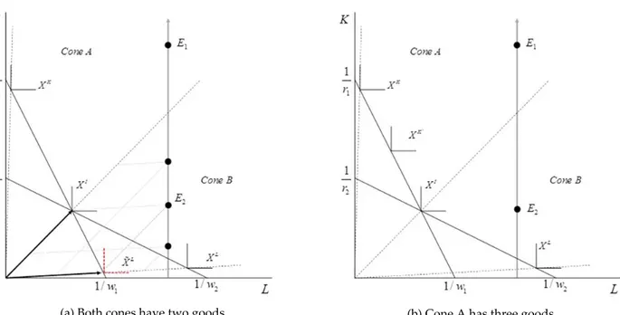
The diagrams shown in Figure 1 depict different goods 



^XL

^,

^XI

^,

^XK



 with their unit‐value  isoquants. The position of the unit‐value isoquants in the K_–L space indicates the relative  input requirements of capital (K_{) and labor (}L_{) to produce a value of output that equals}  one unit of exchange. It also confines the cone of diversification, as shown by the straight  lines through the origin. Isocost lines, tangent to the unit‐value isoquants, indicate the factor  price ratio prevalent in the respective cone of diversification. Countries inhabiting ConeA_, 

5   Empirical support for this assumption is presented in most standard textbooks on growth theory. 

confined by X^I andX^K, have a higher level of capital per worker than countries in ConeB_,  which is confined by X^L andX^I. With constantL, a countryʹs GDP per capita is higher the  farther away its endowment point is from the horizontal axis. 

 

The three endowment points (countries) depicted in Cone Bof Panel (a) rationalize a pattern  of initial diversification and subsequent respecialization. Inside the cone, factor price equali‐

zation (FPE) holds and countries allocate resources so as to produce the two goods X^L and XI. Drawing parallelograms between origin and endowment points indicates the respective  output vectors for the two goods as shown for countryE₂. As drawn here,  E₂

 produces  good  X^L and  X^I in equal share, while the two other countries have a more concentrated  production structure. Because income differences are indicated by the vertical position of the  countries relative to each other, the framework suggests a U‐shaped specialization path  along with increasing GDP per capita. In Cone Ain Panel (a), the high‐income country E₁ is  characterized by a different product mix consisting of  X^I and  X^K. The country’s relative  production structure can be derived in the same way as was done before, but the model does  not yield predictions on the degree of specialization relative to countries inhabiting ConeB.  In other words, the prediction of an inverted U‐shaped diversification path is constrained to  countries residing inside the same cone of diversification. Inside a cone, the model requires  FPE to hold, and a constant set of products implies a diversification pattern at the intensive  margin. Another implication of Panel (a) is that there is no difference in the degree of diversi‐

fication at the extensive margin: at any point (inside a cone of diversification) countries pro‐

duce two goods and trade one good, independent of their stage of development. 

(a) Both cones have two goods  (b) Cone A has three goods 

Figure 1: Lerner Diagrams and Diversification

Based on this approach, Cadot et al. rationalize their identification of a nonmonotone di‐

versification path with the assumption that countries, as they develop, travel from one cone  to another while protecting the industries in which they have lost their comparative ad‐

vantage. For instance, suppose that country E₁ initially resided in the low‐income Cone B_,  where it produced X^L and X^I. As it has become rich, it has found itself in the high‐income  Cone  A_{, where it can no longer produce}X^L. It nevertheless continues to do so by raising  the domestic price (for example, by imposing a tariff or import quota). This is shown by an  inward shift of the unit‐value isoquant to  X^L_{. As also discussed in Bernard, Jensen, and}  Schott (2006), such protectionist measures enable the country to achieve a higher level of di‐

versification at the extensive margin, producing  X^K, andX^I, and  X^L_{. The country re‐}

specializes in the moment when the trade barriers are removed. 

The implication of such a mechanism for the general pattern described in Imbs and  Wacziarg and Cadot et al. would be that almost all countries protect their traditional indus‐

tries during the process of economic development, and that only very few have removed  protectionist barriers. Along these lines, Rodrik (2007) raises concerns about the policy impli‐

cations of increasing levels of diversification among countries that are growing out of pov‐

erty. Pro‐trade policy arguments based on gains from specialization seem to lose their power  if countries are observed to engage in increasing ranges of activities until they reach per capi‐

ta income levels of approximately 22,000 USD (in 2005 purchasing power parity (PPP)).⁶ An  alternative explanation can be obtained by relaxing the assumption that cones of diversifica‐

tion host an equal number of goods. Theories which propose that higher income levels are  reached through (local or global) innovation and product differentiation suggest a positive  correlation between diversification at the extensive margin and levels of GDP per capita (Ac‐

emoglu and Zilibotti 1997; Grossman and Helpman 1991). This is shown in Panel (b) of Fig‐

ure 1, where Cone A now hosts an additional good, X^K', that can be produced only by rich  countries. Diversification now conforms to gains‐from‐trade arguments because countries in  Cone  A specialize in capital‐intensive goods, while countries in Cone  Bproduce labor‐

intensive goods. Nevertheless, high‐income countries produce a wider range of goods. 

2.2  Implications 

Imbs and Wacziarg address the implications of the scenario in Panel (b) in their discussion of  the nonmonotone pattern they identify for production and employment: an inverted U‐

shaped diversification path contradicts standard theories.⁷ Their rationalization is based on  the existence of nontraded goods that become tradable at late stages of economic develop‐

6   This is approximately the turning point, estimated by Cadot et al., where countries begin to respecialize. 

7   Although they do not refer to the Lerner diagram or cones of diversification, they emphasize the fact that di‐

versification requires sufficient resources in order to overcome capital indivisibilities (Acemoglu and Zilibotti  1997). 

ment. That is, while the process of innovation and investment into new activities continuous‐

ly expands the range of the goods produced, countries begin, at some point, to improve their  infrastructure technology. This lowers the cost of trading goods and induces the relocation of  their production to other countries. In countries where respecialization can be observed, the  rate at which nontradable goods become tradable must be higher than the rate at which new  goods are invented and produced. 

It is correct to argue that an improved trade infrastructure, like trade liberalization,  works as a driver of specialization. This argument is also related to an extensive literature on  foreign outsourcing (see, e.g., Feenstra 2010, for an overview). The outsourcing or relocation  of production might even accelerate the diversification process in those (poorer) countries  that “receive” production stages and tasks through this channel.⁸ However, the tradability  argument is vulnerable in two respects. First, it does not bear up against the implication,  stemming from a steady‐state growth rate, that continuous respecialization requires the rate  of trade‐facilitating technological progress to permanently exceed the rate of product discov‐

ery and diversification. Unless this is the case, the pattern of respecialization identified by  Imbs and Wacziarg and Cadot et al. is a temporary phenomenon during a period of global  trade integration rather than a general pattern.⁹ Second, permanence implies that all goods  will be tradable at some point. This brings us back the scenario, depicted in Panel (b) of Fig‐

ure 1, where, all other things being equal, high‐income countries are strictly more diversified  than low‐income countries. To conclude, unless innovation comes to a halt or income differ‐

ences vanish so that all countries inhabit the same cone of diversification, countries continue  to diversify. 

This last statement is the motivation to revisit the empirical evidence, which expects that  diversification at the extensive margin increases monotonically with higher GDP per capita. 

The analysis in this paper concentrates on diversification in exports because the available da‐

ta is more detailed than employment and production data with comparable country and time  coverage. The empirical patterns and theoretical implications revealed by the analysis are as‐

sumed to carry over to production and employment.¹⁰   

 

8   An example is the importance of processing trade for the increase in the skill content of Chinaʹs exports (Amiti  and Freund 2010). 

9   Note that this is also supported by De Benedictis et al.’s (2009) and Parteka’s (2010) findings of continuous di‐

versification when they use relative measures of specialization because they incorporate time effects by con‐

struction. 

10  Although Parteka (2010) finds that concentrations in production and employment do not necessarily move  together, this must be the true for the extensive margin, where relative quantities are neglected and produc‐

tion requires at least a small unit of labor. 

3  Data and Measurement Issues 

This section reproduces Cadot et al.ʹs descriptive analysis and illustrates how their data can  lead to a different conclusion about the diversification–income nexus. Methodological issues  concerning scaling and measurement are discussed alongside this analysis, and a roadmap  with suggestions for the econometric analysis is presented at the end of the section. 

The Cadot et al. data has a panel dimension and reports export‐concentration indices cal‐

culated at the country level based on detailed information from the UN Comtrade database.¹¹  The original data from Cadot et al. covers the years 1988 through 2006 and is used in the first  part  of this  section.  Comparable trade data  from  the  Centre d’Études  Prospectives et  d’Informations Internationales, the CEPII BACI96 data set (Gaulier and Zignano 2010), co‐

vers the years from 1998 through 2009 and is used in the second part. Both data sets are also  applied in the econometric analysis, with the aim of comparing results across different time  periods. 

3.1  Sampling and Scaling 

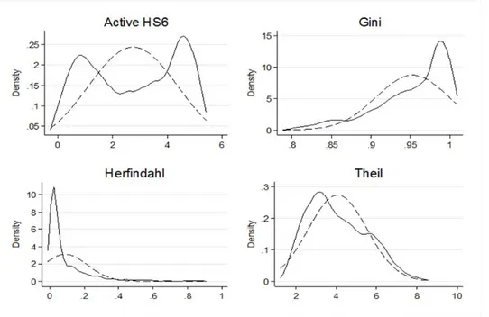
The diversification literature uses alternative concentration measures such as the Gini, Her‐

findahl, or Theil (1972) indices, mainly to show that the results are robust. This subsection fo‐

cuses on the Theil index because it demonstrates the best distributional properties in dis‐

aggregated export data, while its qualitative interpretation is equal to other measures.¹² Ca‐

dot et al. also used it, both to motivate a quadratic parameterization and to identify the ex‐

tensive margin as the relevant dimension of diversification. Panel (a) of Figure 2 reproduces  the diversification path that Cadot et al. show for the Theil index; this is indicated by the two  U‐shaped lines. The solid line represents the predicted pattern of a nonparametric estimation  (locally weighted scatterplot smoothing; LOWESS),¹³ while the broken line reproduces the  prediction of a quadratic polynomial. Both lines suggest a path of initial diversification (i.e.,  decreasing concentration) and subsequent respecialization. The scatterplot shows the under‐

lying sample with all its country–year observations up to an income level of 60,000 USD (PPP  2005).¹⁴ 

11  At the highest level of disaggregation, the UN Comtrade database reports trade flows in about five thousand  product categories using six‐digit codes from the Harmonized System (HS6). 

12  A high index always implies high concentration and a low index always implies low concentration. See Ap‐

pendix A for a discussion of the Gini, Herfindahl, and Theil indices in the present context. 

13  This method is described in greater detail by Imbs and Wacziarg, who apply a modified version of it. 

14  In the figure, as in Cadot et al., the sample is censored at a GDP per capita level of 60,000 USD (PPP 2005). 

Censoring applies only in the graphical representation of the figures, not for the estimations used to obtain  predicted values. This practice follows Cadot et al. and ensures that the predicted path shown here looks the  same as theirs. 

   

Panel (b) of Figure 2 reestimates the parametric and nonparametric curves after removing  countries with populations below one million and those with oil‐export shares greater than  or equal to 50 percent, on average.¹⁵ LOWESS still predicts respecialization, but the quadratic  polynomial is now much more skewed and deviates substantially from the nonparametric  curve. The fact that most of the observations are located near the vertical axis raises the con‐

cern that the quadratic parameterization obtains its pronounced U‐shape from the high vari‐

ation of export concentration in the very first percentiles of the income distribution. Panels  (c) and (d) illustrate the power of a logarithmic transformation. Applied on the horizontal ax‐

is that denotes GDP per capita, it stretches the scale among the lower values. Reestimating 

15  Oil exports are defined as exports in HS chapters 26 and 27. 

(b) Pooled, excl. oil‐ and microstates

(c) Pooled, excl. oil‐/microstates (log GDPpc) (d) Means, excl. oil‐/microstates (log GDPpc)

Figure 2: Theil Index and GDP Per Capita, 1988–2006

Note: Data used is from Cadot et al. (2011). GDP per capita stated in 1,000 international dollars (PPP 2005). Dashed  line: predicted values from quadratic OLS; solid line: LOWESS. Each point represents a country‐year obser‐

vation; ISO codes represent country averages (1988–2006). Micro‐states defined as average population below  one million. Oil exporters defined as average export shares in HS chapters 26 and 27 equal to or greater than  50 percent. 

(a) Pooled, all countries 

1 3 5 7

Theil Index

0 20 40 60

1 3 5 7

0 20 40 60

1 3 5 7

Theil Index

.5 2 8 32

ZAR BDI LBR

MOZ ETH SLE GNB

NER RWA MWIUGACAF

ERI TGO

TZANPL MLI

BGD MDG BFA

GHA KHM TCD

GMB ZMB BEN TJK LSO SDN

LAO KEN SENHTI VNM KGZ

IND MRT

UZB CIV

MDA PNG

PAK CMR

MNG

NIC

CHN GEO

ARM

PHL LKAIDNMAR

HND BOL

JOREGYALB PRY

DOM NAM

SWZ

BIH UKR GTM SLV

TUN COL PER

THA ECU

BLR KAZ

TUR MKD JAM

PAN CRI

BGR MUS

ROM ZAF BRA LBN URY

LVA RUS

MYS CHL

ARG MEXLTU TTO

HRV POL BWA

EST SVKHUNKOR

CZE PRT SVN ISR

NZL

ESP GRCFIN

ITA IRL

GBR SWE FRA DEU HKGJPN AUS

DNK CAN

AUTNLDBEL SGP

CHE USA

NOR

1 3 5 7

.5 2 8 32

the quadratic polynomial and LOWESS with log GDP per capita produces a linear fit on ex‐

port concentration. The similarity of the patterns in panels (c) and (d) suggests that the func‐

tional form obtained from the pooled sample resembles cross‐country differences – that is, a  static pattern. 

Figure 2 illustrates the sensitivity of Cadot et al.’s results with respect to sample selection  and scaling. The downward trend of export concentration at higher stages of economic de‐

velopment and the low number of outliers in panel (d) support the prediction of continuous  diversification discussed in the previous section. The distinction that remains to be made is  that between the intensive and the extensive margin. While the Theil index, like all other  concentration measures, contains information on the shape of a distribution, diversification  at the extensive margin is concerned only with its range. In order to stick to this distinction,  the remainder of the paper measures diversification by counting the number of HS6 prod‐

ucts a country exports. This is the same as analyzing diversification at the extensive margin. 

3.2  The Counting Goods Measure and Its Limits 

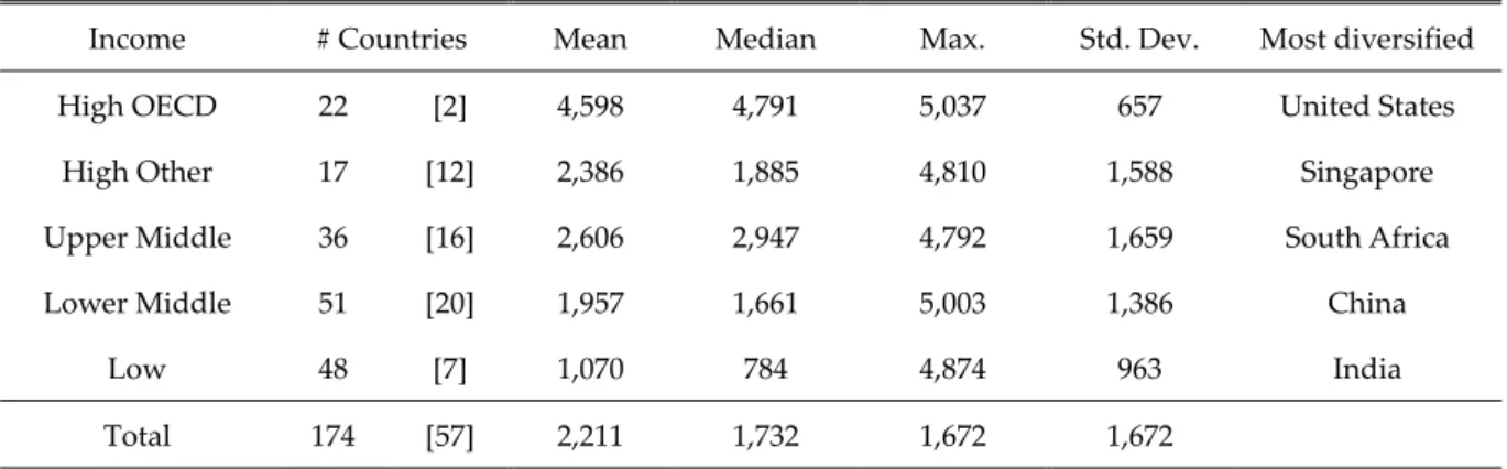
Table 1 shows the average number of goods exported by countries from five different income  groups between 1998 and 2009.¹⁶ The groups vary in size, with most of the observations com‐

ing from low‐income and lower‐middle‐income countries. The figures in brackets indicate  the number of countries that have been removed from the sample because of their small  population or high oil‐export shares. The columns reporting the number of exported goods  by the mean and the median country of a group indicate higher diversification levels for  richer countries. The columns “Max.” and “Std. Dev.” (standard deviation) suggest hetero‐

geneity inside the groups. Four of the five countries that export almost everything are large  economies (China, India, South Africa, and the United States). Singapore, the most diversi‐

fied economy among the high‐income non‐OECD countries, may have reached the high‐

diversification level through its role as a trade hub for other economies.¹⁷ The table does not  contradict the pattern of continuous diversification, but it does reveal potentially important  covariates such as a countryʹs size and geography. 

A similar picture is shown in Figure 3, which suggests a continuous diversification path along‐

side economic development. As in Figure 2, pooled and cross‐sectional data have the same  functional form, independent of whether parametric or nonparametric techniques are used. 

However, the left panel (a) of Figure 3 reveals an aspect that literally points to the limits of  counting goods. The highest level of diversification a country can achieve is, by definition, ex‐

porting all the 5,111 product categories included in the HS6 classification. For coun tries near    

16  The grouping is based on an adjacent file to the CEPII BACI96 data set. 

17  A similar level of diversification can be expected for Hong Kong, which reexports many goods from and to  China (Feenstra and Hanson 2004). 

Table 1: Number of Exported HS6 Products across Income Groups, 1998–2009 

Income  # Countries  Mean  Median  Max.  Std. Dev.  Most diversified 

High OECD  22  [2]  4,598  4,791  5,037  657  United States 

High Other  17  [12]  2,386  1,885  4,810  1,588  Singapore 

Upper Middle  36  [16]  2,606  2,947  4,792  1,659  South Africa 

Lower Middle  51  [20]  1,957  1,661  5,003  1,386  China 

Low  48  [7]  1,070  784  4,874  963  India 

Total  174  [57]  2,211  1,732  1,672  1,672   

Note: The data is drawn from the CEPII BACI96 and represents country averages for 1998–2009. The sample  identifies a total of 5,111 HS6 product categories. Numbers in brackets indicate the number of countries  with a population below one million or oil exports equal to or more than 50 percent of total exports, on  average. Income groups are presented as documented in the CEPII BACI96 adjacent file. 

this limit (practically all the high‐income countries as well as China, India, and Indonesia), it is  impossible to diversify further. Ignoring this limit can lead to downward‐biased estimates  observations for India and China in the upper left of the point cloud in Panel (a) of Figure 3.  

Figure 3: Exported HS6 Lines and GDP Per Capita, 1998–2009 

  (a) Pooled, excl. oil‐/microstates (log GDPpc)   (b) Means, excl. oil‐/microstates (log GDPpc) 

 

Note: GDP per capita stated in 1,000 international dollars (PPP 2005); number of active HS6 lines in 1,000. Dashed  line shows predicted values from quadratic OLS. Solid line shows fitted lines from LOWESS. Each point  represents a country‐year observation; ISO codes represent country averages (1988–2006). Microstates de‐

fined as average population below one million. Oil exporters defined as average export shares in HS chap‐

ters 26 and 27 equal to or greater than 50 percent of total exports (1998–2009). 

Their levels of diversification do not change much despite outstanding growth in the period  shown. Relating these observations to GDP per capita reveals a coefficient close to zero,  while fitting the whole sample suggests a strong positive relationship. Tobin (1958) suggests  censoring those observations that are close to the limit. In the present context this would im‐

ply removing exactly those observations where it is claimed that countries are respecializing. 

Hence, it is useful to have another way to investigate the case of respecialization. 

3.3  Theory, Empirics, and a Roadmap 

The previous subsections presented descriptive evidence for continuous diversification at the  extensive margin. They challenged the case of respecialization and attributed its emergence  to methodological aspects related to the handling of panel data, the distributions of variable  values, and the detail and limits of measurement. In order to obtain an econometric model  that both includes a theoretical rationale and takes into account the data characteristics de‐

scribed in this section, a roadmap for the analysis in Section 4 is briefly outlined here. 

Omitted variables: Parteka and Tamberi (2013) explore several covariates of export di‐

versification in addition to income per capita. Among other things, they find significant ef‐

fects related to exporters’ size and the distance to their markets, as Benedictis et al. (2009)  have suggested. In order to obtain the narrow set of variables needed for the econometric  analysis, it is necessary to derive the gravity equation inherent to the Eaton and Kortum  model. When aggregated to the total exports of a country and related to the extensive mar‐

gin, its implementation is analogous to Baldwin and Harrigan’s (2011) assessment of export  zeros and unit values across space. 

Sample selection: An assumption of the comparative statics analyzed in Section 2 is that  countries differ only in their level of capital per worker and are otherwise symmetric. The  gravity equation accounts for asymmetries arising from differences in country size and geog‐

raphy. However, policy barriers – another important determinant of diversification – can be  manifold and are difficult to control for (Anderson and Van Wincoop 2004). To cope with  this, this paper uses a subsample of open economies based on Wacziarg and Welch’s (2008)  classification for comparison. Oil exporters and small countries always remain outside the  sample. 

Limited dependent variables: The upper limit in the HS6 data leads to the observation  that many countries stop diversifying, which may wrongly suggest a turning point (especial‐

ly when the log‐transformation of GDP per capita is omitted). Censoring observations near  the upper limit helps to avoid potential estimation bias but also removes those observations  for which this paper claims that respecialization does not occur. Evidence on US import data  from Feenstra, Romalis and Schott (2002) is thus used to back up the results obtained from  using the HS6 data. The US data includes a much richer set of products and encompasses  more than 10,000 categories. Although examining exports to the United States narrows the 

scope of the analysis to a single export destination, this approach provides an increased level  of detail and no country reaches the upper limit within the period under study.¹⁸ 

4  Econometric Analysis 

This section extends the analysis undertaken in Section 2 and presents the theoretical frame‐

work upon which the econometric analysis is based. 

The framework relies on the Eaton and Kortum model to derive a gravity equation for  diversification. This equation is used in the empirical analysis in the second part of this sec‐

tion. Alternative levels of aggregation and time periods are considered in order to check the  robustness of the results. Dynamic methods are then applied to infer the direction of causali‐

ty. 

4.1  Export Diversification and Technology Differences 

The Eaton and Kortum model features an arbitrary number of countries 

i   1, , N

 and  goods

j   1, , J

. Consumers in country 

n

 decide to purchase good  j at the lowest availa‐

ble price pn

 

j ^min



pni

 

j i^;  ^{1, ,}N



. The setup is as follows: 

Prices include unit production costs, ( / ) c z , and trade costs,

d

,

  ⁿⁱ

 

i

 

^{i ni}

^,

p j c d

z j

 

    

where d_ni 

1

 and d_nn

1

. Unit production costs fall with productivity  z j_i

( )

, which is ran‐

domly drawn from a cumulative distribution function (CDF). The shape of this distribution  is governed by a parameter, 



, that quantifies gains from trade that result from comparative  advantage. The location of the CDF – or the average z j_i

( )

 – is indicated by T_i and denotes a  countryʹs overall technological development.¹⁹ When comparing two countries, the one with  a higher T  is likely to also have a higher z j_i

( )

, hence it has an absolute advantage. 

The probability 



 that a country i can successfully export to 

n

 – that is, offer the lowest  price – is a function of its technology, its factor costs c_i, and transportation costs between the  two countries, relative to the rest of the world: 

18  Only six of 144 countries exported more than 10,000 goods to the United States during the sample period  1989–2006. In descending order, with the number of observations in parentheses: Canada (16), Germany and  the United Kingdom (12), Italy (8), China (7), and Japan (1). 

19  Technology can also include broader concepts such as infrastructure, institutions, and other non‐sector‐related  determinants of efficiency. 

(1.1) 

1

( )

( ) .

i i ni

ni N

k k nk

k

T c d T c d





^ 









 

Eaton and Kortum show that this expression is equivalent to iʹs share of the total expendi‐

ture of country 

n

_, 

(

X_ni

/

X_n

)

, so that 

(1.2) 

 

n

Φ ,

i i ni n

ni

T c d X X



  

where  _n



^N_k1T c d_k

(

_{k nk}

)

^ 

(

p_n

/ ) 

^{ resembles the} denominator of the previous equa‐

tion and also determines the price level in the destination market. That is, if the rest of the  world has a low level of technology or high factor prices and delivery costs, the price level in  country 

n

 will be high, making it easier for country i to offer the lowest price. 

Substituting terms and summing over all destinations yields the total sales of country i  as a function of its technology, factor costs, and a term that summarizes the interaction be‐

tween (deflated) delivery costs and market size: 

(1.3) 

1

1 1

/ .

i

N N

ni

i ni i i n

n n n

R

X X T c d X

p













 



 

   

 

 



 

In empirical adaptations, the sum of partners’ GDP‐weighted distances is interpreted as the  remoteness of a country, R_i, which (inversely) indicates proximity to large markets. In other  words, the more remote a country is, the farther it is from large markets and the lower its  probability of being a successful exporter to any country. Dividing the last equation by an  analogous expression for country k and taking logs states the log‐linear gravity equation for  countries’ relative exports. 

(1.4)  ln ⁱ ln ⁱ ln ⁱ ln ⁱ

k k k k

X T c R

X T



c R

       

  

       

        

The comparative expression emphasizes that when a time dimension is added to all varia‐

bles, a country can improve its technology but still export less if other countries have experi‐

enced greater technological growth. Likewise, if technology improves in all countries at an  equal pace, relative exports remain unchanged. This aspect has to be borne in mind when the  equation is applied to panel data.²⁰ An implication of the model can be quoted directly from  Eaton and Kortum (2002: 1748) in order to emphasize the relation of their model to the this  paper’s argument: “A source with a higher state of technology, lower input cost [sic], or low‐

er barriers exploits its advantage by selling a wider range of goods.” Hence, the model not  only yields a gravity equation (which can also be obtained from other theories) but also pre‐

20  In a cross‐section this problem does not arise because absolute and relative technology differences cannot be  distinguished with only one observation per country. 

dicts that countries diversify at the extensive margin because 



Xi^/ Xk



¹ always implies  that i should export a wider range of goods than k.²¹ 

4.2  Baseline Estimation 

The estimation equation takes the following form: 

(1.5) 

6 2

1 2 3 4

6

ln ln ln ln

HS

it it it it i

HS it

t t t t t

N y y

N y y L R

L R

 

^{ }



^{ }



^{ }



^{ }



          

         

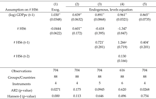
Compared to (1.4), variables vary over time, t, and time averages replace the benchmark  countryk, with x_t 



x_it /N. The dependent variable is not logged because its distribution  is not as extreme as the income per capita data (it is similar to that in Figure 3). The variables  of the Eaton and Kortum model are interpreted in the same way as in Baldwin and Harri‐

gan’s (2011) analysis of US export zeros and unit values across space.²² They are proxied with  GDP per capita,  y, population size, L_, and a measure for remoteness, R_{. GDP per capita}  reflects the level of technology and its squared term is included to see if there are nonlineari‐

ties beyond the asymptotics internalized by taking logs. Population proxies factor costs,  which are lower in large countries due to the internal factor competition.²³ Remoteness is cal‐

culated as in Baldwin and Harrigan (2011), capturing the size‐weighted distance from desti‐

nation markets.²⁴ The expected qualitative results are ˆ₁0, ˆ₂ 0, ˆ₃ 0, and ˆ₄ 0.  Given the similarity of pooled and cross‐sectional patterns documented in the previous  section, the baseline estimates use both ordinary least squares (OLS) and the between effects  (BE) estimator as a starting point. The latter is used instead of a single cross‐section for an ar‐

bitrary year and takes country averages for the entire sample period. Using the BE estimator  in disaggregated trade data has the advantage that it averages out unstable export spells that  would otherwise be fully included in a single year. The resulting year‐selection bias (which  has the same attenuating effect as measurement error) can be meaningful, especially among  low‐ and middle‐income countries, which frequently engage in trade relationships that do  not survive longer than one or two years (i.e., high churning rates; Besedes and Prusa 2006; 

21  Eaton and Kortum note this property as a key difference from other models. With monopolistic competition,  adjustments take place at the intensive margin because consumers will always generate demand for all goods. 

22  Note that they are interested in the destination marketʹs characteristics and particularly in the effect of dis‐

tance. As shown in the previous subsection, this variable becomes part of the exporterʹs remoteness when bi‐

lateral exports are aggregated to total exports. 

23  Baldwin and Harrigan (2011) argue that large countries have a higher level of domestic competition because  they must sell a great deal and are therefore often their own lowest‐cost suppliers. 

24  E.g. 

1

1

.

N

n i

n ni

R GDP

distance





 

 





  Note that in my data, values are R_i1bn because the GDP data used for calcula‐

tion was scaled in 1‐USD units. 

Eaton, Eslava, Kugler, and Tybout 2007). As discussed at the end of Section 3, alternative  samples are also estimated to see how robust the results are. Additionally, a reduced model  with  only  GDP  per  capita  as  the  explanatory  variable  is  estimated: 



N_it^HS6

/

N_t^HS6



 

 

1

ln ^

y_it

/

y_t

^





2

ln ^

y_it

/

y_t

^

²



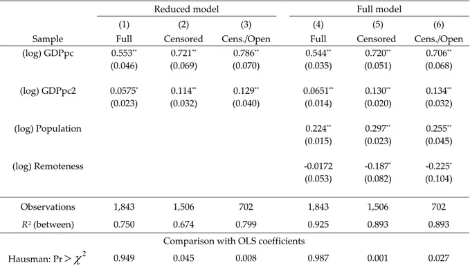
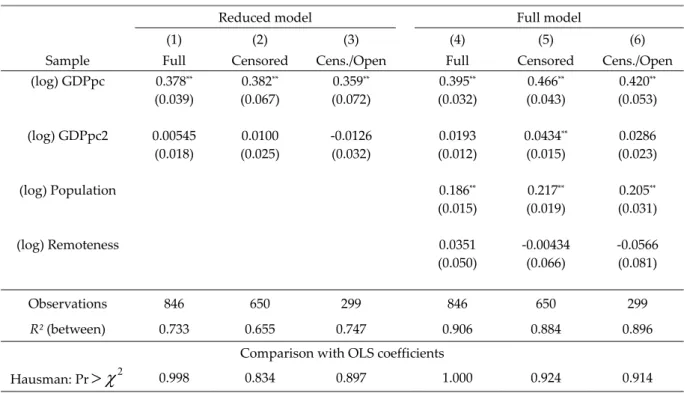
_{it. The  next} subsection proceeds with  further specification tests. 

Main results: Table 2 presents the BE results in two panels. The first panel, columns (1) to  (3), reports the results of the reduced model, while the second panel, columns (4) to (6),  shows results for the full model as stated in (1.5). The first column of each panel uses the full  range of data (except oil‐exporting countries and microstates); censored samples in columns  (2) and (5) use only observations up to a limit of 4,500 goods; and columns (3) and (6) are fur‐

ther restricted to open economies. As expected, censoring affects the results in that the  squared GDP per capita variable becomes insignificant. All other coefficients reveal the ex‐

pected signs, although remoteness is significant only in the censored samples. The full model  produces a higher R‐squared than the reduced model, but the inclusion of population and  

 

Table 2: Active HS6 Lines and GDP Per Capita, 1998–2009; BE Estimation 

  Reduced model    Full model 

  (1)  (2)  (3)    (4)  (5)  (6) 

Sample  Full  Censored  Cens./Open    Full  Censored  Cens./Open  (log) GDPpc  0.255^**  0.227^**  0.251^**    0.228^**  0.277^**  0.257^** 

  (0.030)  (0.049)  (0.047)    (0.023)  (0.032)  (0.032) 

               

(log) GDPpc2  ‐0.0222^a  ‐0.0245  ‐0.0305^a    ‐0.0285^**  ‐0.00976  ‐0.0143 

  (0.012)  (0.015)  (0.018)    (0.007)  (0.009)  (0.011) 

               

(log) Population          0.177^**  0.200^**  0.173^** 

          (0.013)  (0.016)  (0.023) 

               

(log) Remoteness          ‐0.0550  ‐0.148^**  ‐0.170^** 

          (0.045)  (0.053)  (0.057) 

               

Observations  1,404  1,082  475    1,404  1,082  475 

R² (between)  0.730  0.676  0.810    0.897  0.879  0.925 

Comparison with OLS coefficients 

Hausman: Pr



²  0.962  0.635  0.728    0.994  0.937  0.992 

Source: The table shows estimation results using data drawn from the CEPII BACI96 and CEPII Gravity dataset, and the World Development Indicators database. Standard errors in parentheses; ^a p < 0.1, ^* p < 0.05, ^** p <

0.01. All variables are normalized by their annual means. Sample excludes oil exporters and microstates.

Observations with exported HS6 lines equal to or greater than 4,500 have been censored in columns (2), (3), (5), and (6).