Alternating Offer Bargaining Experiments with Varying Institutional Details

Alternating Offer Bargaining Experiments with Varying Institutional Details ^∗

Vital Anderhub

, Werner Güth

, Nadège Marchand

Abstract

The game theoretic prediction for alternating offer bargaining depends crucially on how “the pie” changes over time, and whether the proposer in a given round has ultimatum power. We study experimentally eight such bargaining games. Each game is once repeated before moving on to the next one what defines a cycle of altogether16 successive plays. Participants play three such cycles. There are no major experience effects but strong and reliable effects of anticipated rule changes. The latter, however, are not due to strategic considerations but rather to the social norms of fairness and efficiency.

∗We thank Dorothea Kübler and Claude Montmarquette for helpful comments.

†Humboldt-University of Berlin, Department of Economics, Institute for Economic Theory III, Spandauer Str. 1, D-10178 Berlin, Germany

‡Groupe d’ Analyse et de Théorie Economique (GATE), UMR 5328 du CNRS, 93, Chemin des Mouilles, 69130 Ecully, France and CIRANO, 2020 rue University, 25ème étage, Montréal (Québec) H3A 2A5, Canada; marchann@cirano.umontreal.ca

1. Introduction

Alternating offer bargaining is a familiar topic in experimental economics. Start- ing with Binmore, Shaked, and Sutton (1985) the late eighties experienced a vivid debate whether and how actual bargaining behavior differs from game theoretic predictions (see Güth, 1995, and Roth, 1995, for surveys). Almost invariantly these studies assume a “shrinking pie”, i.e. that delaying an agreement is costly.

What was varied more systematically was the time horizon T, i.e. the last pe- riod for reaching an agreement, varying from T = 1 (Güth et al., 1982), T = 2 (Binmore et al.,1985, Güth and Tietz, 1986, Ochs and Roth,1989),T = 3 (Ochs and Roth, 1989), T = 5 (Neelin et al., 1988) to “T = ∞”, i.e. to not specifying explicitly afinal periodT (Weg, Rapoport, and Felsenthal, 1990) as suggested by Rubinstein (1982). One major result of these studies is that only for T = 1 and T = 2 the implications of backward induction are obvious even when this does not always imply the corresponding behavior. ForT >3, strategic considerations are more of the forward induction type¹. Since the influence of the time horizon T has already been thoroughly explored, our experiment always relies onT = 3.

The fact that parties alternate in proposing an agreement does not necessarily imply that bargaining has to end in the last period T if no earlier agreement is reached. If there is commitment power at all (what is implicitly assumed by all bargaining models), it seems feasible that one always can declare one’s offer to

be final, i.e. has ultimatum power (Güth, Ockenfels, and Wendel, 1993). In our

experiment participants confront both situations, those where each proposer has ultimatum power and those where bargaining can stop early only by an early agreement.

Over time the “pie”, i.e. what can be distributed among the parties, can either decrease or increase. Whereas a shrinking pie reflects the well-known costs of delaying an agreement like waste of time, starting too late cooperating etc., an

1One such argument is, for instance, to demand the difference between the1st and 2nd round pie in round1if this yields more than 50 % of the1st round pie.

increasing pie can be justified by the fact that later agreements are often more adequate, e.g. by being based on more information, superior incentives etc. Here we do not only rely on monotonic developments but explore also a “hill” (the

“pie” is largest in period 2) and a “valley” (the “pie” is lowest in period 2).

A vector (p1, p2, p3) of pies pt in periods t = 1,2,3 is numerically specified for each of the four (the two monotonic and the two non-monotonic) different “pie”- developments.

Each of the four vectors (p1, p2, p3)is playedfirst twice with and then twice with- out ultimatum power. Thus participants first learn to play a usual alternating offer game before commanding ultimatum power already in the earlier periods (t= 1 andt= 2). We refer to the altogether 16 games (4 vectors (p1, p2, p3)×4 successive plays) as a cycle. Participants play three such cycles, i.e. altogether48 bargaining games.

How behavior is influenced by past results is intensively studied, both theoreti- cally (in evolutionary game theory and economics) and experimentally (see Roth and Erev,1995, for a selective overview). By letting participants play many times the same simple or more complex (e.g. Huck, Normann, and Oechsler,1999) game one observes how behavior adapts to previous experiences in an otherwise con- stant environment. Here we also study such “behavioral adaptation” but restrict experiences with the same game to 6 plays and with the same vector (p1, p2, p3) to12 plays.

Contrary to many theoretical models of behavioral adaptation (see Weibull,1995, for a survey) boundedly rational decision making is influenced by past experiences (the shadow of the past) and by deliberating the likely consequences of the various choice alternatives (the shadow of the future). Especially boundedly rational decision makers should deliberately react to a changing environment, represented by switching from one of the8games to another. “Robust learning experiments”

(see Güth, 2000, for a comparison with other studies) do not study behavior in one game but in a variety of related games. The idea is to collect evidence for learning (in the sense of improving behavioral parameters in the light of past experiences)

and for cognitive adjustments when confronting a new situation. In the light of such evidence one hopefully can try to model how learning and forward looking deliberation interact in a process of boundedly rational decision emergence. Unlike perfect rationality bounded rationality should not be based on abstract axioms but rather on sound empirical facts. The latter can be provided by explorative and hypotheses testing (robust learning) experiments.

With this background in mind we can summarize the main intentions of our experimental study:

• We want to establish (stylized) facts and a data basis illustrating how bound- edly rational negotiators learn from previous experiences with the same or a closely related bargaining game.

• We want to demonstrate that the likely consequences of bargaining behavior are anticipated but not in a perfectly rational way, as suggested by backward induction, but rather in a norm-guided way.

• If the largest “pie” requires to delay an agreement, efficiency (in the sense of reaching an agreement when the pie is largest) requires a lot of trust that one will not be exploited. Our experimental data should reveal whether the fear of being exploited questions efficiency and whether such a fear is justified.

Our results are straightforward: Participants mostly reach an agreement when the pie is largest and they share this pie rather equally (slightly favoring the proposer in this period). Especially in case of universal ultimatum power this often contradicts game theory. Partly unfair offers are used to discourage inefficient agreements. Regarding the first two aspects this shows, that learning is of no or little importance and that, in simple environments like ours, norm guided deliberation is crucial.

In the following section 2 we first introduce the 8 games and their benchmark solutions. Section 3 is devoted to details of the experimental procedure. Section 4 describes the main results and section 5 statistically corroborates our main results.

Section 6 concludes.

2. The game variety

Two bargaining parties, players 1 and 2, alternate in proposing an agreement which the other can then accept or reject. Acceptance ends the game with the proposed payoffdistribution, a vector(u1, u2)withpt ≥u1,u2 ≥0andu1+u2 =pt

where the pie pt is what can be distributed in period t = 1,2,3. If t < T and the offer pt−dt to the other party (dt is what the proposer demands for himself) is not an ultimatum, rejection leads to periodt+ 1 where nowpt+1 can be allocated by the rejecting party. If t=T or if, fort < T, the offerpt−dt is an ultimatum, rejection implies conflict with each party receiving0-payoff. Acceptance, of course, implies that the proposer receives dt and the responder pt−dt. In period

t= 1: player 1chooses d1, i.e. 1 proposes, 2responds, t= 2: player 2chooses d2, i.e. 2 proposes, 1responds, t= 3: player 1chooses d3, i.e. 1 proposes, 2responds.

If one disregards different individual time preferences as, for instance, studied by Ochs and Roth (1989) the “pie”-development for T = 3 can be described by the vector (p1, p2, p3)of “pies” pt specifying in German Mark (DM) what can be distributed in period t = 1,2,3. We rely on the four vectors (p1, p2, p3) listed in Table II.1.

p1 p2 p3 nickname symbol

30 20 10 decline D

10 20 30 increase I

10 25 10 hill H

25 10 25 valley V

Table II.1: The four “pie”-developments

Each of the four vectors D, I, H and V can be played with proposers having ultimatum power, the games D^y, I^y, H^y, and V^y, or not, the games Dⁿ,Iⁿ, Hⁿ, andVⁿ. For each of the4vectorsD,I,H, andV (the4rows in Table II.2) the left

column of Table II.2 describes the solution demands (d^∗₁, d^∗₂, d^∗₃) and their payoff implicationsu^∗₁ andu^∗₂ for player1and2when only integer offers are possible and an indifferent responder always rejects. If ultimatum power is available, it will always be used, i.e. each proposal d^∗_t for t = 1,2,3 and the games D^y, I^y, H^y, andV^y is an ultimatum. Thus with ultimatum power bargaining always stops in period t = 1 whereas this is true only for D if no ultimatum power is available.

The periodt^∗ in which the agreement is reached² is indicated in Table II.2 by fat demandsd^∗_t. Whereas in then-gamesDⁿ,Iⁿ, Hⁿ, and Vⁿ the outcome is always efficient in the sense thatu^∗₁ andu^∗₂ add up to the maximal “pie”, this is only true for the y-games D^y andV^y when p1 is largest.

ultimatum power (p1, p2, p3)-type n(o) y(es)

d^∗₁ d^∗₂ d^∗₃ u^∗₁ u^∗₂ d^∗₁ d^∗₂ d^∗₃ u^∗₁ u^∗₂ D= (30,20,10) 19 10 9 19 11 29 19 9 29 1 I = (10,20,30) 10 20 29 29 1 9 19 29 9 1 H = (10,25,10) 10 15 9 10 15 9 24 9 9 1 V = (25,10,25) 24 10 24 24 1 24 9 24 24 1

Table II.2: The solution demands d^∗₁,d^∗₂,d^∗₃ and payoffsu^∗₁, u^∗₂ for the 8 different games D^y,I^y, H^y, V^y, respectively Dⁿ, Iⁿ,Hⁿ, Vⁿ

3. Experimental procedure

The computerized experiment involved 6 sessions, 5 with 12 participants and 1 with 10. Participants, mostly students of economics or business administration of Humboldt University−Berlin, were invited by leaflets to register for the ex- periment. They were seated at visually isolated terminals where they found the written instructions (see Appendix A for an English translation). After read- ing them carefully participants could privately ask for clarifications. Then the experiment started with the first cycle.

2The agreement period t^∗ for gameVⁿ where player 1can achieve the same agreement in period 1 and 3 is left ambiguous in spite of our requirements (according to our assumptions player2should reject thefirst offer and accept the second one in periodt= 3where acceptance is the only best reply).

A cycle consists of two plays of Dⁿ , followed by two plays of D^y, and continuing with this pattern for the vector I, H, and V with four plays each. This cycle of altogether 16 rounds was twice repeated. After each round participants were randomly rematched without switching roles (of player 1, respectively 2). Thus a participant usually confronted 6 different partners in an irregular fashion. Average earnings are DM 32.9 including the DM 5,−show up-fee. A session needed about 110 minutes (30 minutes for reading the instructions and answering questions).

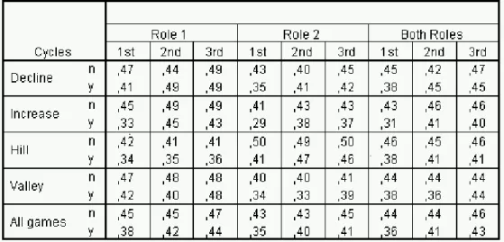
More detailed information about monetary payoffs is contained in Table IV.1 where earnings are separated according to role (player 1 and 2), game type and cycle.

4. Results

One coarse way of searching for experience effects is to compare the average rela- tive (to the maximal pie) earnings of both players for the three cycles (see Table IV.1which distinguishes by roles,1or 2, cycle (1^st, 2^nd, 3^rd), pie vector (D, I, H, V, all) and n(o)ory(es)−ultimatum power). Relative earnings are surprisingly con- stant over the three cycles when proposers command no ultimatum power. We only found significant differences in the y−games’ relative earnings between cy- cles.³ When comparing relative earning variations in and between cycles, we found significant increases only for the Declinepie-development with ultimatum power (between the1^st cycle (rounds3and4)and the 3^rd cycle (rounds35 and36) and between these two cyclesp=.0008,Binomial test, one-tailed, for all tests).

For then−games the distribution of relative earnings in the 3^rdcycle is not signif- icantly different from those in cycles1and 2 withp=.479for player1(Wilcoxon Matched-Pairs Signed Ranks Test, one-tailed), resp. p = .479 for player 2. For they−games one obtains significant differences withp=.0001 andp= .0001 for player 1, resp. 2. This suggests

3Statistically one compares fori = 1,2the differences in average relative (to the maximal pie) earnings between cycles separately for each of the 4 games (with ultimatum power). These test results are, of course, questionable since they assume independence in spite of repeated interaction.

Table IV.1: Average earnings as shares of max{p1, p2, p3} separated by game type, role and cycle.

Observation 1: Only in the more complex y−games one has to learn how to reach efficient agreements.

Average earnings are affected by

• the conflict rate

• the period of reaching an agreement

• the payoff distribution which is accepted.

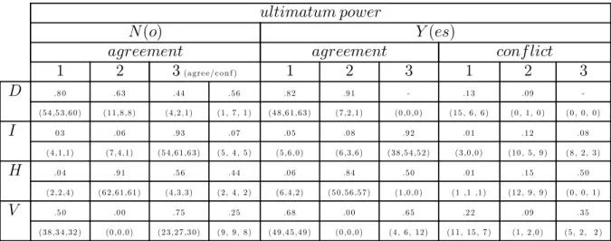
The first aspect is illuminated by Table IV.2 listing the agreement, respectively conflict ratios as well as their absolute numbers (for the three cycles) separately for the n(o) and the y(es)−games and the periods t = 1,2,3. Most agreements occurred when the periodic pie is largest, (in case of ”V(alley)” this applies to the 1^st and 3^rd period). Remember that game theory excludes conflict and predicts agreement for games with the largest periodic pie except for the gamesI^y andH^y (see Table II.2). The agreement ratios in Table IV.2 thus imply

Observation 2: Agreement is mostly achieved when the pie is largest what partly (for games I^y andH^y) rejects game theory.

ultimatum power

N(o) Y(es)

agreement agreement conf lict

1 2 3(a g re e / c o n f ) 1 2 3 1 2 3

D ^{.8 0 .6 3 .4 4 .5 6 .8 2 .91 - .13 .0 9 -}

(5 4 ,5 3 ,6 0 ) (1 1,8 ,8 ) (4 ,2 ,1) (1, 7 ,1) (4 8 ,61,6 3 ) (7 ,2 ,1) (0 ,0 ,0 ) (15 , 6 , 6 ) (0 ,1, 0 ) (0 , 0 , 0 )

I ^{0 3 .0 6 .9 3 .0 7 .0 5 .0 8 .9 2 .01 .12 .0 8}

(4 ,1,1) (7 ,4 ,1) (5 4 ,61,6 3 ) (5 , 4 , 5 ) (5 ,6 ,0 ) (6 ,3 ,6 ) (3 8 ,5 4 ,5 2 ) (3 ,0 ,0 ) (10 , 5 , 9 ) (8 , 2 , 3 )

H ^{.0 4 .91 .5 6 .4 4 .0 6 .8 4 .5 0 .01 .15 .5 0}

(2 ,2 ,4 ) (6 2 ,61,61) (4 ,3 ,3 ) (2 , 4 , 2 ) (6 ,4 ,2 ) (5 0 ,5 6 ,5 7 ) (1,0 ,0 ) (1,1,1) (12 , 9 , 9 ) (0 , 0 ,1)

V ^{.5 0 .0 0 .7 5 .2 5 .6 8 .0 0 .6 5 .2 2 .0 9 .3 5}

(3 8 ,3 4 ,3 2 ) (0 ,0 ,0 ) (2 3 ,2 7 ,3 0 ) (9 , 9 , 8 ) (4 9 ,4 5 ,4 9 ) (0 ,0 ,0 ) (4 , 6 ,12 ) (1 1,15 , 7 ) (1, 2 ,0 ) (5 , 2 , 2 )

Table IV.2: Conditional probability of reaching an agreement or conflict (only for ultimatum power) in period t (total number of 1^rst,2^nd, 3^rd cycle in brackets).

Participants are, however, not simply efficiency-minded as shown by the non neg- ligible numbers of conflicts 28 for D^y, 40 for I^y, 34 for H^y and 45 for V^y when proposer have ultimatum power (for no ultimatum power the frequencies of con- flict are 9 for Dⁿ, 14 for Iⁿ, 6 for Hⁿ and 26 for Vⁿ). Conflicts often, but not always decrease with experience, as measured by cycle (see conflict frequencies in brackets, Table IV.2). Unlike to the n−games conflict in y−games can result earlier or later: Like agreements they result more frequently in period t when pt

is largest, i.e. when one would have expected a fair offer. More specifically, com- paring the conflict ratios in games D^y andV^y (where p1 is largest) with those in games I^y andH^y yields significant differences (p=.047 Wilcoxon Matched-Pairs Signed Ranks Test, one-tailed, forD^y versus I^y andp=.023for V^y versus H^y).⁴

Observation 3: Only for game types D^y and V^y when the 1^st pie is largest, conflict occurs most frequently in the 1^st period of games with ultimatum power (for the other y−games conflict is delayed). Without ultimatum power the pie developmentV inspires the most conflicts (in all three cycles).

4We only compare those two games whose maximal pie-values are the same.

Since efficiency of agreements depends only weakly on the level of experience (as measured by cycle), Table IV.3 provides a fair overview of the efficiency rate

δ = u1+u2

max{p1, p2, p3}

of agreements for all 8 game types (cases of conflict are excluded). Ultimatum power of proposers hardly affects efficiency of agreements even in games I^y and H^y where the game theoretic benchmark solution predicts δ = ¹₃, respectively δ = ²₅. Also the differences between pie-dynamics are minor (≤.07).

The agreed upon distributions usually favor slightly the player who is the proposer for the largest pie, as revealed by player1’s payoff shares

s = u1

u1+u2

of agreements listed in Table IV.3. Only the pie dynamics “H(ill)” with player 2 as the proposer when the pie is largest yields a share s < .5. If one compares the s−share in games Hⁿ and H^y with that of the other games, the (negative) difference is highly significant; similar comparisons between the other games reveal no significant effects. This is qualitatively in line with the benchmark solution for Hⁿ (with s^∗ =.4). Altogether the results in Table IV.3 suggest

Observation 4: Agreements are nearly always efficient, i.e. reached in periods t whenptis largest, and favor slightly (by a not more than 5% deviation from the equal split) the proposer in that period t.

N(o) Y(es) (δ, s) (δ, s) D (.93,.52) (.98,.54) I (.96,.53) (.93,.54) H (.95,.46) (.96,.45) V (1,.54) (1,.55)

Table IV.3 : Efficiency and relative payoff distribution δ and s when conflict is avoided.

ultimatum power

(p1, p2, p3)-type n(o) y(es)

d₁ d₂ d₃ u₁ u₂ d₁ d₂ d₃ u₁ u₂ D= (30,20,10) 16.5 11.2 6.7 14 12.8 16.9 9.5 13.8 11.7 I = (10,20,30) 8 13.2 16.2 14.3 12.6 8 12.9 16.2 12 10.5 H = (10,25,10) 7.3 13.8 5.9 10.3 12.4 7.3 14.4 7 8.8 11.2 V = (25,10,25) 14.3 7.0 14 11.9 10 14.1 6.8 13.9 10.8 8.8 Table IV.4: The average demands and payoffs observed for the 8 different games

D^y, I^y, H^y, V^y, respectivelyDⁿ, Iⁿ, Hⁿ, Vⁿ (fat entries when pt is largest)

Table IV.4 corresponds to Table II.2. The striking difference is that extreme allo- cations with u^∗₂ = 1 are completely avoided. For the n−games the actual results are at least qualitatively in line with the effects, suggested by the benchmark so- lution.⁵ Iny−games where the benchmark solution always predicts meager offers (pt−dt = 1) it cannot account at all for the actual behavior. Minor differences are due to the differences in conflict ratios and in degrees of missing an agreement when the pie is largest.

According to Table IV.4 the average offers on the way to the period with the maximal pie can be quite meager: So the average demands d1 in period 1for the vector I are with 80% of p1 rather unfair; for period 2 it is with 66% for Iⁿ and 64.5% for I^y still above the level54% in period 3 when the pie is maximal. Also for the vector H the average demand in period 1 is with 73% much higher than the average demanded share 55.2% (for Hⁿ), resp. 57.6% (for H^y) in period 2 with the largest pie. The average demanded sharesd2 for the vectorV are slightly more moderate (70 % for Vⁿ, 68% for V^y). Also after missing an agreement for the largest pie (in periods t= 2and 3 for Dand in period t= 3 forH) the offers are quite generous.

Observation 5: The desire to reach an agreement when the pie is largest is signaled, respectively induced by meager offers in earlier periods, both in n−games and in y−games (in the latter games an additional signal is, of course, not to use ultimatum power).

5That most agreements for Vⁿ are reached in period t = 1 only questions the special as- sumption for the case of indifference.

This last observation is corroborated by Figure IV.1which plots the relative offers at periods t= 1,2,3. The bold line links the relative offers made when the pie is largest (unlike in Table IV.3 here the rejected offers are included). For the largest pie-periods mean relative offers stay in the narrow interval [.38;.47] whereas the mean relative offers for given rounds t fluctuate a lot. Participants, who fail to reach an agreement at the highest pie period (D and H games), propose often higher relative counter offers in the next period (in 31.25% of the cases).

0,0 0,1 0,2 0,3 0,4 0,5 0,6

1 4 7 10 13 16 19 22 25 28 31 34 37 40 43 46

Ro u n d s

Relative offers

p er io d t =1 p erio d t =2 p er io d t =3 t =m ax {p 1 ,p 2 ,p 3 }

Figure IV.1: Average relative offers at periodt= 1,2,3 andt=max{p1, p2, p3} over rounds.

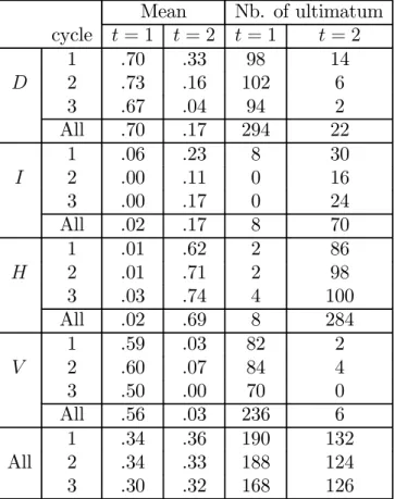
The ways in which an agreement can be reached when pt is largest differ for n− andy−games. In an n−game the proposer in that period t <3 must suggest an (by the responder in t) acceptable distribution of pt. In a y−game the proposer can additionally exclude any further possibility to reach an agreement by declaring the offer to befinal. Do proposers iny−games rely on the same mechanism as in n−games? Table IV.5 displays the rates (and the absolute numbers) of exercising one’s ultimatum power separately for t = 1 and t = 2 (int = 3 every offer is an ultimatum offer), the four pie-developments, and each cycle. Around 70% of the offers pt−dt when pt is largest are ultimatum offers. Thus ultimatum power is not just neglected but consistently used:

Observation 6: Contrary to game theory ultimatum power is not always exer- cised but mainly used to encourage acceptance whenpt is largest.

Altogether our data suggest that commitment power, here in the sense of ulti- matum power, is largely overrated by game theory. At least the desire to strive for fair and efficient agreements seems to be much more influential. The latter conclusion is supported by Table IV.4 listing average payoffs (with never differ by more than 2.5, i.e. |u1−u2|<2.5).

Mean Nb. of ultimatum cycle t = 1 t= 2 t= 1 t= 2

1 .70 .33 98 14

D 2 .73 .16 102 6

3 .67 .04 94 2

All .70 .17 294 22

1 .06 .23 8 30

I 2 .00 .11 0 16

3 .00 .17 0 24

All .02 .17 8 70

1 .01 .62 2 86

H 2 .01 .71 2 98

3 .03 .74 4 100

All .02 .69 8 284

1 .59 .03 82 2

V 2 .60 .07 84 4

3 .50 .00 70 0

All .56 .03 236 6

1 .34 .36 190 132

All 2 .34 .33 188 124

3 .30 .32 168 126

Table IV.5 : Termination options (rates and frequencies) chosen at periods t= 1,2.

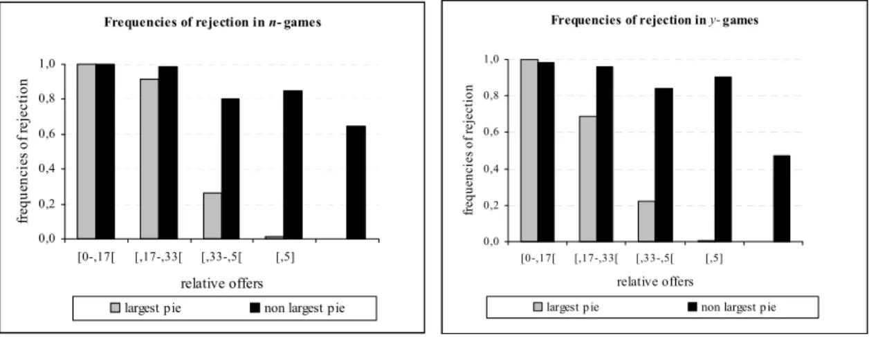
Let S denote the share of pt which has been offered. In general, a low share S should go along with a high rejection rate. A low offered share S must, however, not be an attempt to exploit the responder.If pt is not the largest pie, it may be simply a signal to wait for the larger pie. In Figure IV.6a andb we illustrate for

n− and y−games as well as for the largest and non largest pies the frequencies of rejected offers for different intervals for S, namely 0 ≤ S ≤ .17, .17 < S ≤ .33, .33< S < .5, .5≤S ≤.5, .5< S. Clearly, only for the largest pie-periods the usual relation between the fairness and acceptability of S holds.

Observation 7: Only in the largest pie period the rejection rate decreases with the relative share S which has been offered.

Frequencies of rejection in n-games

0,0 0,2 0,4 0,6 0,8 1,0

[0-,17[ [,17-,33[ [,33-,5[ [,5]

relative offers

frequencies of rejection

largest pie non largest pie

Figure IV.6 a

Frequencies of rejection in y-games

0,0 0,2 0,4 0,6 0,8 1,0

[0-,17[ [,17-,33[ [,33-,5[ [,5]

relative offers

frequencies of rejection

largest pie non largest pie

Figure IV. 6b

5. Further Statistical Analysis

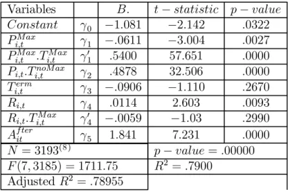
To illustrate how the previous observations are supported by our data, we have run a linear regression explaining the offer behavior. The offer made to subject i at periodtwithi= 1, ...,70andt = 1,2,3is estimated by the following equation⁶:

Oit =γ₀+ (γ₁+γ⁰₁.T_it^{M ax})P_it^{M ax}+γ₂Pit.T_it^{noM ax}+γ₃T_it^erm+ (γ₄+γ⁰₄.T_it^Max)Ri,t+γ₅A^{f ter}_it

The variable P_it^{M ax} is the largest pie, i.e. P_it^{M ax} = max{p1it, p2it, p3it}. T_it^{M ax} (T_it^noMax)represents a dummy variable taking value of1(0)ifPit,the pie for which

6As participants alternate their position of proposer and responder during the round, offer Oit is made by participants in role1at periodt= 1andt= 3and by participants in role 2 for t= 2.

subject i makes an offer at period t, is (not) largest and 0(1) otherwise. T_i,t^erm is also a dummy variable with T_it^erm = 1 for y−games and T_it^erm = 0for n−games.

Variable Ri,t indicates the round corresponding to observation Oit. A^{f ter}_it is a dummy variable with value 1 when period t follows the largest pie period and 0 otherwise. In case of thepie−development D one would have A^{f ter}_it = 1for t = 2 and in case of H fort = 3.

To test the significance of Observation 5 that efficient agreement are induced meager offers in early periods parameter γ₁, estimating the influence of P_it^{M ax}, should be significantly negative and parameterγ⁰₁, concerning the combined effect of P_it^Max, be significantly positive. Since Observation 6 claims that the termina- tion option is not used to exploit but rather to reach an efficient agreement, the influence of the termination option on offers should be negative but insignificant.

Furthermore, this should not significantly increase the number of conflicts. To trace learning effects we analyse separately the influence of time Rit on offers when the pie is largest (γ⁰₄T_it^{M ax}Rit) and when not (γ₄Rit). The low level of learn- ing in average relative earnings (Observation 1) does not exclude learning effect in offer behavior.⁷

The regression result is listed in Table V.1. Overall, our model is highly significant (p−value = .00000 and R² = .7900) The expected effects due to Observation 5 are significantly confirmed: P_i,t^{M ax} has a negative and highly significant overall effect on offer behavior (γ₁ < 0) in the non-maximal pie-periods and increases significantly offers in the maximal pie-period(γ⁰₁ >0).

Observation 6 is weakly in line with the regression results since ultimatum power implies only insignificantly smaller offers in y−games (γ₃ < 0). Offers increase significantly over time (γ₄ > 0) and decrease only insignificantly when t is the largest pie period (γ⁰₄ > 0). This latter result is in line with Observation 6. In case of A^{f ter}_it = 1 participants, who rejected in the largest pie period, make a counter offer. Their reactions are captured by parameter γ₅ which is positive and significant. Such counter offers are relatively higher to avoid delaying the agreement even more or not reaching one at all.

7Participants might have learned to increase their offers and to avoid conflict more often so that on the agregate level earnings remain stable on average.

Variables B. t−statistic p−value Constant γ₀ −1.081 −2.142 .0322 P_i,t^{M ax} γ₁ −.0611 −3.004 .0027 P_i,t^{M ax}.T_i,t^{M ax} γ⁰₁ .5400 57.651 .0000

Pi,t.T_i,t^{noM ax} γ₂ .4878 32.506 .0000

T_i,t^erm γ₃ −.0906 −1.110 .2670

Ri,t γ₄ .0114 2.603 .0093

Ri,t.T_i,t^{M ax} γ⁰₄ −.0059 −1.03 .2990

A^{f ter}_it γ₅ 1.841 7.231 .0000

N = 3193⁽⁸⁾ p−value=.00000 F(7,3185) = 1711.75 R² =.7900

Adjusted R² =.78955

Table V.1: Estimation results of the regression.

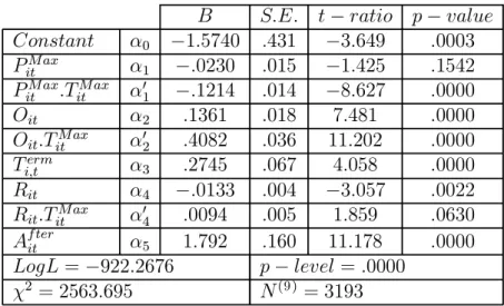
Acceptance behavior can be similarly explained by a probit regression in which the dependent variableyitis coded into{0,1}to estimate the probability of acceptance (yit= 1) by subject i in period t with t = 1,2,3 and i = 1, ..,35 (a rejection is coded as yit = 0). We denote by Oit the offer to whichyit reacts.

yit =α0+ (α1+α⁰₁.T_it^{M ax}).P_it^{M ax}+ (α2+α⁰₂.T_it^Max).Oi,t+α3T_it^erm+ (α4+α⁰₄.T_it^{M ax})Ri,t+α5A^{f ter}_it

The estimation results, reported in Table V. 2, show that the overall model is significant. The probability of acceptance increases significantly with the offer made (α2 > 0) and even more if this is the largest pie period (α⁰₂ > 0). The highly significant and negative parameter α⁰₁ reveals that the overall probability of conflict is larger in the largest pie period: Participants are not simply efficiency minded (see the non-negligeable numbers of conflict in Table IV.2) and do more likely reject in the largest pie period. According to the positive and significant parameter α5 they later on are more inclined to accept. Ultimatum power helps to reach an agreement (α3 >0, p−level =.0000) confirmingObservation 6.Over time, the probability of acceptance decreases significantly, i.e. responders learn to reject.

8Our regression takes 3193 observations into account instead of the 5040 theoretical ones due to agreements in earlier periods (fort <2andt <3).

B S.E. t−ratio p−value Constant α0 −1.5740 .431 −3.649 .0003 P_it^{M ax} α1 −.0230 .015 −1.425 .1542 P_it^{M ax}.T_it^{M ax} α⁰₁ −.1214 .014 −8.627 .0000

Oit α2 .1361 .018 7.481 .0000

Oit.T_it^{M ax} α⁰₂ .4082 .036 11.202 .0000 T_i,t^erm α3 .2745 .067 4.058 .0000 Rit α4 −.0133 .004 −3.057 .0022 Rit.T_it^{M ax} α⁰₄ .0094 .005 1.859 .0630

A^{f ter}_it α5 1.792 .160 11.178 .0000

LogL=−922.2676 p−level =.0000 χ² = 2563.695 N⁽⁹⁾ = 3193

Table V. 2: Estimation results of Probit Regression Model.

6. Discussion and conclusions

In typical experiments of alternating offer bargaining participants are confronted with just one pie-development and (except for Güth, Ockenfels and Wendel,1993) with ultimatum power only in the last period t = T. Compared to this our participants faced 4 very different types of pie-dynamics as well as early (t≤ T) and only late (t = T) ultimatum power. By exploring the broader spectrum of institutions/rules we could demonstrate that participants

• are motivated by efficiency considerations, i.e. aim at reaching an agreement when the pie is largest, and

• use unfair offers mainly as a signal that an agreement should be reached when the pie is largest,

• are reluctant to exploit ultimatum power regardless when it is available.

Compared to other studies of robust learning (see Güth, 2000) this leaves little or no room for learning. This suggests the more general conclusion that learning, i.e.

9cf. note 2.

shadow of the past, is negligible when strong norms like efficiency and equality concerns provide strong guidance how to negotiate.

Forward looking deliberation seems to be decisive. The main intentions, namely to share the maximal pie and to propose a rather fair distribution, reveal carefully deliberated plans and thus a much stronger shadow of the future than of the past.

The results for the games I^y and H^y nevertheless reveal that normative game theory, which is purely forward looking, does not explain experimentally observed behavior (compare the predictions in Table II.2 with the results in Table IV.4).

The forward looking considerations of the participants are rather norm oriented than strategic: Behavior is shaped by fairness and efficiency concerns and not by opportunistic rationality.

It would, however, be premature to generalize our conclusions beyond the scope of distribution conflicts in small groups like dyads. Other situations, e.g. large anonymous markets, might trigger more egoistic motives and lead to outcomes which are more in line with opportunistic rationality. Although each robust learn- ing experiment like ours covers already a variety of structurally different institu- tions, one should perform similar studies for other types of decision problems (see the studies reviewed in Güth, 2000).

References

[1] Binmore, K., A. Shaked, and J. Sutton (1985): Testing noncooperative bar- gaining theory: A preliminary study, American Economic Review, 75 (5), 1178 - 1180.

[2] Güth, W. (1995): On ultimatum bargaining - A personal review, Journal of Economic Behavior and Organization, 27, 329 - 344.

[3] Güth, W. (2000): Robust learning experiments - Evidence for learning and deliberation, Working Paper, Humboldt-University of Berlin.

[4] Güth, W., R. Schmittberger, and B. Schwarze (1982): An experimental anal- ysis of ultimatum bargaining, Journal of Economic Behavior and Organiza- tion, 367 - 388.

[5] Güth, W. and R. Tietz (1986): Auctioning ultimatum bargaining positions - How to act if rational decisions are unacceptable?, in: Current Issues in West German Decision Research, R. W. Scholz (ed.), Frankfurt, 173 - 185.

[6] Güth, W., P. Ockenfels, and M. Wendel (1993): Efficiency by trust in fair- ness? - Multiperiod ultimatum bargaining experiments with an increasing cake, International Journal of Game Theory, 22, 51 - 73.

[7] Huck, S., H.-T. Normann, and J. Oechssler (1999): The indirect evolutionary approach to explaining fair allocations, Games and Economic Behavior 28, 13 - 24.

[8] McKelvey, R. D. and T. R. Palfrey (1992): An experimental study of the centipede game, Econometrica, 60, 803 - 836.

[9] Neelin, J., H. Sonnenschein, and M. Spiegel (1988): A further test of nonco- operative bargaining theory: Comment, American Economic Review, 78 (4), 824 - 836.

[10] Ochs, J. and A. E. Roth (1989): An experimental study of sequential bar- gaining,American Economic Review, 79 (3), 355 - 384.

[11] Roth, A. E., Erev, I. (1995): Learning in Extensive-Form Games : Experi- mental Data and Simple Dynamic Models in the Intermediate Term ,Games and Economic Behavior, vol.8, pp. 164-212.

[12] Roth, A. E. (1995): Bargaining experiments, in: Handbook of Experimental Economics, J. H. Kagel and A. E. Roth (eds.), Princeton, N.J.: Princeton University Press, 253 - 348.

[13] Rubinstein, A. (1982): Perfect equilibrium in a bargaining model,Economet- rica, 50, 97 - 109.

[14] Weg, E., A. Rapoport, and D. S. Felsenthal (1990): Two-person bargaining behavior infixed discounting factors games with infinite horizon,Games and Economic Behavior, 2 (1), 76 - 95.

[15] Weibull, J. W. (1995): Evolutionary game theory, Cambridge and London:

M.I.T. Press.

Appendix A:

In the experiment you will interact anonymously in groups of two participants. Each partcipant gets 5 DM show up fee. You will not be informed about the other’s identity nor will your partner be informed about yours. You and your partner constitute a group of two persons namedAandB. WhatAandBcan share is an amount of points,p(20 points =1DM), whose value depends on when you and you partner reach an agreement.

The interaction is organized as follows:

1. In the first period,t = 1, Partner A chooses an offerO1 to Partner B. If Partner B accepts the offer, A earns p1 −O1 and B earns O1. If not, they go to the second periodt= 2.

2. In the second period, t= 2, Partner B chooses an offerO2 to PartnerA. If Partner Aaccepts the offer,B earnsp2−O2andAearnsO2. If not, they go to the third period t= 3.

3. In the third period,t = 3, Partner A chooses an offer O3 to PartnerB. If Partner B accepts the offer, Aearns p3−O3 and B earnsO3. If not, both earn 0.

The valuesp1, p2 and p3 depend on the situationD, I, H orV:

p1 p2 p3 Situation

30 20 10 D

10 20 30 I 10 25 10 H

25 10 25 V

In addition, you might have a Termination Option.

Termination Option : If one partner chooses the termination option in period t < 3, the interaction process ends with this offer, i.e. the other cannot make a counteroffer.

Partner A can choose the Termination Option in t = 1, and partner B in t = 2. If

A chooses the termination option, partnerB can’t choose it in the next period as the interaction stops in periodt = 1regardless whetherB accepts or not.

You will be 4 times in situation D (twice without and twice with the Termination Option), then 4 times in situation I (twice without and twice with the Termination Option), then 4 times in situation H (twice without and twice with the Termination Option), 4 times in situationV (twice without and twice with the Termination Option).

The whole session consists of 3 sequences of such16 rounds, i.e. of altogether 48 rounds.

At the beginning of each round, we form randomly new groups of two participants with oneA and oneB participant.

After each round you will be informed about your own earning. Payments will be made privately at the end of the session. Please, raise your hand if you have any question.

We will try to answer them privately. Thank you for your cooperation!

Appendix B:

Please, fill out this questionnaire completely. To check your understanding of the in- structions we kindly ask you to answer the following questions. Suppose the following arbitrarily specified decisions:

2. In periodt= 2, the offer equalsO2 = 5and Aaccepts it.

How much doesA and B participants earn?

A earns In situation D,

B earns

A earns In situation I,

B earns A earns

In situation H,

B earns

A earns In situation V,

B earns

3. Imagine that partnerAchooses the termination option in period t= 1. Can PartnerB make a counteroffer in periodt= 2?

Yes No