Adaptive methods for risk calibration

Adaptive Methods for Risk Calibration

DISSERTATION

zur Erlangung des akademischen Grades doctor rerum politicarum

(Doktor der Wirtschaftswissenschaft) eingereicht an der

Wirtschaftswissenschaftlichen Fakult¨at der Humboldt-Universit¨at zu Berlin

von

M. Sc Weining Wang geboren am in

Pr¨asident der Humboldt-Universit¨at zu Berlin:

Prof. Dr. Jan-Hendrik Olbertz

Dekan der Wirtschaftswissenschaftlichen Fakult¨at:

Prof. Dr. Ulrich Kamecke Gutachter:

a. Prof. Dr. Wolfgang Karl H¨ardle b. Prof. Dr. Vladimir Spokoiny

Tag des Kolloquiums: 2nd August 2012

Acknowledgements

Completing a PhD degree together with my master is a four-year and fruitful journey. I learned a lot on doing research and presenting results from it as well as on how to communicate and cooperate with people in the scientific community. I must greatly acknowledge my coauthors, teachers, and colleagues, who shared a lot of their experiences.

My first gratitude goes to my principal advisor, Dr. Wolfgang Karl H¨ardle. His influence on me is majorly on scientific research motivation. He provided me with the statistics vision and artistic thinking. He is good at motivating students to work hard and offered various opportunities to attend scientific conferences and workshops. He also made me connected with many world renowned scholars, from whom I gained inspirations for research and for life. He has been a strong and supportive adviser to me throughout my graduate school, while I can still have great freedom to pursue independent work.

Special thanks goes to the other advisor Dr. Vladimir Spokoiny for his mathe- matical insights and advice on structuring and editing paper. His enthusiasm and endurance in developing original and elegant statistical theorems inspired me a lot. I want to also thank Dr. Ya’acov Ritov for his ideas and inspirations, and for him being a role model for me as a statistician.

I am also grateful to Dr. Ostap Okhrin, Dr. Yarema Okhrin, Dr. Martin Oden- ing, Dr. Brenda L´opez Cabrera, Dr. Ihtiyor Bobojonov, Dr. Jianqing Fan, Dr.

Philippe Rigollet, Dr. Lixing Zhu, Dr. Cheng-Der Fuh for their shared wisdoms.

Their guidance is very helpful and I owe them my heart-felt appreciation.

Members of LvB chair of stastistics, and WIAS also deserve my sincerest thanks, their friendship and assistance has meant more to me than I could ever express.

Meanwhile, I could not complete my work without the financial support from the Deutsche Forschungsgemeinschaft via SFB 649 “Economic Risk”, Humboldt- Universit¨at zu Berlin.

My friends in US, Taiwan and other parts of the world were sources of laughter, joy, and support. I wish to thank my family, my father, mother, grandfather, aunt and specially to my husband, Wei Cui. Their love provided me with inspiration and was my driving force. I sincerely wish I could show them just how much I love and appreciate them.

Contents

1 Introduction 3

2 Local quantile regression 6

2.1 Introduction . . . 6

2.2 Adaptive estimation procedure . . . 8

2.2.1 Quantile regression model . . . 8

2.2.2 A qMLE View on Quantile Estimation . . . 9

2.2.3 Local polynomial qMLE . . . 10

2.2.4 Selection of a Pointwise Bandwidth . . . 11

2.2.5 Parameter Tuning by Propagation Condition . . . 13

2.3 Simulations . . . 16

2.3.1 Critical Values . . . 16

2.3.2 Comparison of Different Bandwidth Selection Techniques . . 18

2.4 Applications . . . 22

2.5 Finite Sample Theory . . . 28

2.5.1 Modeling Bias . . . 28

2.5.2 “Oracle” Property . . . 30

2.6 Conclusion . . . 30

2.7 Appendix . . . 31

2.7.1 Uniform concentration of the MLEs eθ_k(x) . . . 32

2.7.2 Uniform quadratic approximation of the local excess . . . 33

2.7.3 Theorem for critical values . . . 39

2.7.4 Propagation Property and Stability . . . 42

2.7.5 Proof of the “oracle” property . . . 42

3 Tie the straps: uniform bootstrap confidence interval for additive

models 44

3.1 Introduction . . . 44

3.2 Additive models and bootstrap confidence sets . . . 47

3.2.1 Coupled Bootstrap for Quantiles . . . 49

3.2.2 How does the coupling work? . . . 50

3.3 Main Results . . . 51

3.4 Simulation . . . 53

3.4.1 Additive model . . . 56

3.5 Empirical analysis . . . 57

3.5.1 Firm expenses analysis . . . 57

3.5.2 The impact on stock market . . . 58

3.6 Conclusion . . . 61

3.7 Appendix . . . 61

3.7.1 Proof of Theorem 3.1 . . . 61

3.7.2 Proof of Theorem 3.2 . . . 64

4 Hidden Markov structures for dynamic copulae 68 4.1 Introduction . . . 68

4.2 Model Description . . . 70

4.2.1 Incorporating HAC into HMM . . . 70

4.2.2 Likelihood estimation . . . 73

4.3 Theoretical Results . . . 75

4.4 Simulation . . . 76

4.4.1 Simulation I . . . 77

4.4.2 Simulation II . . . 81

4.5 Applications . . . 81

4.5.1 Application I . . . 81

4.5.2 Application II . . . 87

4.6 Conclusion . . . 92

4.7 Appendix . . . 92

4.7.1 Copulae . . . 92

4.7.2 Proof of Theorems 4.3.1 and 4.3.2 . . . 93

5 Localising temperature risk 100 5.1 Introduction . . . 100

5.2 Model . . . 104

5.2.1 How does the adaptation work? . . . 105

5.3 Empirical analysis . . . 110

5.4 Forecast and comparison . . . 125

5.5 A temperature pricing example . . . 129

5.6 Conclusions and further work . . . 132

Bibliography 141

List of Figures

2.1 The bandwidth sequence (upper panel), plot of data and the esti- mated 90% quantile curve (lower panel) . . . 7 2.2 Demonstration of the local adaptive algorithm. . . 13 2.3 The bandwidth sequence (upper left panel), the smoothed band-

width (magenta dashed); the data with noise (grey, lower left panel), the adaptive estimation of 0.75 quantile (dashed black), the quan- tile smoother with fixed optimal bandwidth = 0.06 (solid black), the estimation with smoothed bandwidth (dashed magenta); box- plot of block residuals fixed bandwidth (upper right), adaptive band- width (lower right) . . . 19 2.4 The bandwidth sequence (upper left panel), the smoothed band-

width sequence (dashed magenta); the observations (grey, lower left panel), the adaptive estimation of 0.75 quantile (dotted black), the true curve (solid black), the quantile smoother with fixed optimal bandwidth = 0.063 (dashed dotted blue), the estimation with adap- tively smoothed bandwidth (dashed magenta); the blocked error of the adaptive estimator (lower right); the fixed estiamtor (upper right). 20 2.5 The adaptive estimation of first derivative of the above quantile

function (left panel grey), the true curve (solid black), the estima- tion with smoothed bandwidth (dashed black), the quantile smoother with fixed optimal bandwidth = 0.045 (dotted black); the blocked error of the adaptive estimator (lower right); the fixed estiamtor (upper right). . . 21

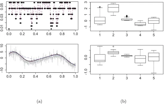
2.6 The bandwidth sequence with smoothed bandwidth curve(upper left panel), the smoothed bandwidth (dashed magenta); Scatter plot of stock returns (upper right panel), the adaptive estimation of 0.90 quantile (solid magenta), the quantile smoother with fixed opti- mal bandwidth = 0.15 (dotted black); fixed bandwidth curve (dot- ted black), adaptive bandwidth curve (grey), the estimation with smoothed bandwidth (dashed magenta), confidence band (dashed black) (lower left panel); adaptive bandwidth with normal scale (lower right). . . 24 2.7 The bandwidth sequence with smoothed bandwidth curve (upper

left panel); Scatter plot of stock returns (upper right panel), the adaptive estimation of 0.90 quantile (red), the quantile smoother with fixed optimal bandwidth = 0.19 (dotted black); fixed band- width curve (dotted black), adaptive bandwidth curve (grey), con- fidence bands (dotted dashed black) (lower left panel); adaptive bandwidth with normal scale (lower right panel) . . . 25 2.8 The adaptive trend curve (grey), smoothed adaptive curve (dashed

black), estimation with fixed bandwidth (dotted black). τ = 0.90 . 26 2.9 Plot of quantile curve for standardized weather residuals over 40

years at Berlin, 95% quantile, 1967−2006 . Selected bandwidths (upper), observations with estimated the quantile function (middle), the estimated the quantile function (lower). . . 26 2.10 Estimated 90% quantile of variance functions, Berlin, average over

1995−1998 , 1999−2002 (red), 2003−2006 (green) . . . 27 2.11 Estimated 90% quantile of variance functions, Kaoshiung, average

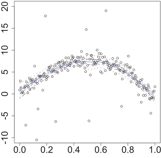
over 1995−1998 , 1999−2002 (red), 2003−2006 (green) . . . 28 3.1 Plot of true curve (grey), robust estimation and band (blue dashed),

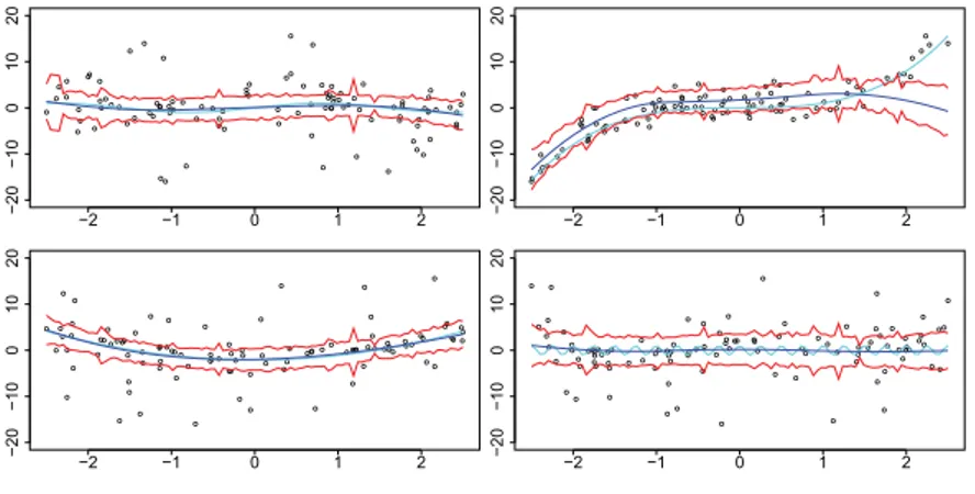
local polynomial estimation (black), bootstrap band (red dotted) . . 55 3.2 Plot of true curve (dark blue), robust estimation and bands (cyran),

bootstrap band (red dotted) . . . 57 3.3 Robust estimation (blue), bootstrap band (red dotted), left up:

Log(Asset), right up: Leverage, left below: Age, right below: TOPTEN. 59 3.4 Robust estimation (blue), bootstrap band (red dotted), Y: S&P

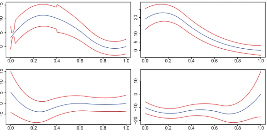
index, left up: exchange rates EUR-USD, right up: crude oil price, left below: inflation index, right below: real estate price. . . 60

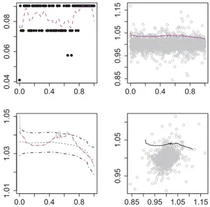
3.5 Robust estimation (blue), bootstrap band (red dotted), Y: S&P index log return, left up: exchange rates EUR-USD, right up: crude oil price, left below: inflation index, right below: real estate price. . 60 4.1 LCP for exchange rates: structure (upper) and parameters (lower,

θ1(green) andθ2)(blue) for Gumbel HAC. m0 = 40. . . 70 4.2 Graphical representation of the dependence structure of HMM, where

Xt depends only on Xt−1 and Yt only onXt. . . 71 4.3 The underlying sequence xt (upper left panel), marginal plots of

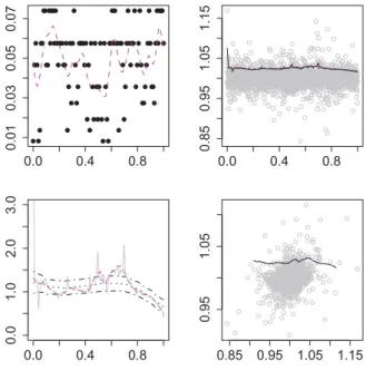
(y_t1, y_t2, y_t3). . . 78 4.4 Snapshots of pairwise scatter plots of dependency structures (t =

500, . . . ,1000), the (yt1) vs. (yt2) (upper), the (yt2) vs. (yt3) (mid- dle), and the (yt1) vs. (yt3)(lower). . . 79 4.5 The convergence of states (upper panel), transition matrix (middle

panel), and parameters (lower panel). Estimation starts from near the true value (red); starts from values provided by our proposal (blue) . . . 80 4.6 The convergence of states (upper panel), transition matrix (middle

panel), parameters (lower panel). Estimation starts from near true value (red); starts from values attained by our proposal (blue) . . . 82 4.7 The error of misidentification of states from 100 samples . . . 83 4.8 Rolling window estimators of Pearson’s (left) and Kendall’s (right)

correlation coefficients between the GARCH(1,1) residuals of ex- change rates: JPY and USD (solid line), JPY and GBP (dashed line), GBP and USD (dotted line). The width of the rolling window is set to 250 observations. . . 84 4.9 Rolling window for exchange rates: structure (upper) and depen-

dency parameters (lower, θ1 and θ2) for Gumbel HAC. w = 250.

. . . 85 4.10 HMM for exchange rates: structure (upper) and dependency pa-

rameters (lower, θ1 and θ2) for Gumbel HAC. . . 86 4.11 Plot of estimated number of states . . . 86 4.12 Map of Guangxi, Guangdong, Fujian in China . . . 89 4.13 Log-survivor-function (red) and 95% prediction intervals (blue) of

the simulated distribution for the fitted model with sample log- survivor-function superimposed (black) . . . 91 4.14 . . . 98

4.15 Fully and partially nested copulae of dimension d = 4 with struc- tures s= (((12)3)4) on the left and s= ((12)(34)) on the right . . . 99 5.1 Kernel density estimates (left panel), Log normal densities (middle

panel) and QQ-plots (right panel) of normal densities (gray lines) and Kaohsiung standardised residuals (black line) . . . 101 5.2 Upper panel: Kaohsiung daily average temperature (black line),

Fourier truncated (dotted gray line) and local linear seasonality function (gray line), Residuals in lower part. Lower left panel:

Fourier seasonal variation (Λbt) over time. Lower right panel: Kaoh- siung empirical (black line), Fourier (dotted gray line) and local linear (gray line) seasonal variance (bε²_t) function. . . 103 5.3 Localised model selection (LMS) . . . 107 5.4 Map of locations where temperature are collected . . . 111 5.5 The empirical (black line), the Fourier truncated (dotted gray line)

and the the local linear (gray line) seasonal mean (left panel) and variance component (right panel) using Quartic kernel and band- width h= 4.49. . . 113 5.6 Simulated CV for likelihood of seasonal volatility (5.7) withθ^∗ = 1,

r= 0.5,M C = 5000 withα= 0.3 (gray dotted line), 0.5 (black dot- ted line), 0.8 (dark gray dotted line) (left), with different bandwidth sequences (right). . . 115 5.7 Estimation of mean and variance for Kaohsiung. In each figure se-

quence (also smoothed for volatility) of bandwidths (upper panel), nonparametric function estimation (solid grey line), with fixed band- width (dashed line), adaptive bandwidth (dot-dashed line) and smoothed adaptive bandwidth (dotted line) (bottom panel of each figure). . . 116 5.8 Estimation of mean and variance for New-York. In each figure se-

quence (also smoothed for volatility) of bandwidths (upper panel), nonparametric function estimation (solid grey line), with fixed band- width (dashed line), adaptive bandwidth (dot-dashed line) and smoothed adaptive bandwidth (dotted line) (bottom panel of each figure). . . 117 5.9 Estimation of mean and variance for Tokyo. In each figure sequence

(also smoothed for volatility) of bandwidths (upper panel), nonpara- metric function estimation (solid grey line), with fixed bandwidth (dashed line), adaptive bandwidth (dot-dashed line) and smoothed adaptive bandwidth (dotted line) (bottom panel of each figure). . . 118

5.10 Estimation of mean and variance for Berlin. In each figure sequence (also smoothed for volatility) of bandwidths (upper panel), nonpara- metric function estimation (solid grey line), with fixed bandwidth (dashed line), adaptive bandwidth (dot-dashed line) and smoothed adaptive bandwidth (dotted line) (bottom panel of each figure). . . 119 5.11 QQ-plot for standardised residuals from Berlin using different meth-

ods. . . 121 5.12 150 days ahead forecast, true temperature (black dots), adaptive

method (red dots), Diebold method (blue dots), fitted using 2 years data. . . 127 5.13 150 days ahead forecast, true temperature (black dots), adaptive

method (red dots), Diebold method (blue dots), fitted using 3 years data. . . 128 5.14 MPR for Berlin CAT futures and Tokyo AAT futures traded before

measurement period. . . 131

List of Tables

2.1 Critical Values with different r and α . . . 17

2.2 Critical Values with Different τ . . . 17

2.3 Critical Values with Different Bandwidth Sequences . . . 17

2.4 Critical Values with Different Noise Distributions . . . 18

2.5 Critical Values with Different Noise Distributions in Local Linear Case . . . 18

2.6 Comparison of Monte Carlo errors, averaged over 1000 samples . . . 22

2.7 Comparison of error mis-specification, errors are calculated averaged over 1000 samples . . . 22

2.8 Summary of deviation from normality . . . 23

2.9 P-values of Normality Tests:Berlin . . . 28

2.10 P-values of Normality Tests:Kaoshiung . . . 29

3.1 Averaged coverage probabilities and areas of nominal asymptotic (bootstrap) with 100 repetitions per sample, and 200 samples. . . . 55

3.2 Simulated coverage probabilities and areas of nominal (bootstrap) with 100 repetitions per sample, and 200 samples. . . 58

4.1 VaR backtesting results,α, where “Gum” denotes the Gumbel cop-b ula and “RGum” the rotated Gumbel one. . . 87

4.2 Robustness relative to AW(DW) . . . 88

4.3 Rainfall occurrence probability and shape, scale parameters esti- mated from HMM (data 1957–2006) . . . 90 4.4 True correlations, simulated averaged correlations from 1000 sam-

ples their 5% confidence intervals. 1 Fujian, 2 Guangdong, 3 Guangxi 90

5.1 ADF and KPSS-Statistics, coefficients of the autoregressive pro- cessAR(3) and continuous autoregressive modelCAR(3) model for the detrended daily average temperatures time series for different cities. +0.01 critical values, * 0.1 critical value, **0.05 critical value,

***0.01 critical value. . . 111 5.2 Seasonality estimates Λbt of daily average temperatures in Asia.

All coefficients are nonzero at 1% significance level. Data source:

Bloomberg. . . 112 5.3 Skewness, kurtosis, Jarque Bera (JB), Kolmogorov Smirnov (KS)

and Anderson Darling (AD) test statistics (365 days) of corrected residuals. . . 114 5.4 AR(L) parameters for Berlin (20020101-20071201), Tokyo (20030101-

20081201), New-York (20030101-20081201) and Kaohsiung (20030101- 20081201) using joint/separate mean (JoMe/SeMe) with fixed band- width curve (fi), adaptive bandwidth curve (ad), adaptive smoothed bandwidth (ads) seasonal mean/volatility (Me/Vo) curve. . . 122 5.5 ps-values of Jarque Bera (JB), Kolmogorov Smirnov (KS) and An-

derson Darling (AD) test statistics for Berlin (20020101-20071201)

& Kaohsiung (20020101-20071201) corrected residuals under differ- ent adaptive localizing schemes: for joint/separate mean (JoMe/SeMe) with fixed bandwidth curve (fi), adaptive bandwidth curve (ad), adaptive smoothed bandwidth (ads) seasonal mean/volatility (Me/Vo) curve. . . 123 5.6 p-values of Jarque Bera (JB), Kolmogorov Smirnov (KS) and Ander-

son Darling (AD) test statistics for New-York (20030101-20081201)

& Tokyo (20030101-20081201) corrected residuals under different adaptive localising schemes: for joint/separate mean (JoMe/SeMe) with fixed bandwidth curve (fi), adaptive bandwidth curve (ad), adaptive smoothed bandwidth (ads) seasonal mean/volatility (Me/Vo) curve. . . 124 5.7 Averaged Cumulative Square Error and its confidence interval of

the forecast from 1000 samples. . . 126 5.8 Normality Statistics . . . 126 5.9 Weather futures listed on date (yyyymmdd) at CME (Source: Bloomberg)

andFbt,τ1,τ2,λ,θ estimated prices with MPR (λt) under different local- isation schemes (θbunder SeMe Locave, SeMe Locsep, SeMe Loc- max), P(Put), C(Call) . . . 133

5.10 Root Mean Squared Error (RMSE) between the CME and the esti- mated weather futuresFb_{t,τ1,τ2,λ,θ} under different localisation schemes (θbunder SeMe Locave, SeMe Locsep, SeMe Locmax) . . . 134

Chapter 1

Introduction

This article includes four chapters. The first chapter is entitled “Local Quan- tile Regression”, and its summary: Quantile regression is a technique to estimate conditional quantile curves. It provides a comprehensive picture of a response contingent on explanatory variables. In a flexible modeling framework, a specific form of the conditional quantile curve is not a priori fixed. This motivates a local parametric rather than a global fixed model fitting approach. A nonparametric smoothing estimate of the conditional quantile curve requires to balance between local curvature and stochastic variability. In the first essay, we suggest a local model selection technique that provides an adaptive estimate of the conditional quantile regression curve at each design point. Theoretical results claim that the proposed adaptive procedure performs as good as an oracle which would minimize the local estimation risk for the problem at hand. We illustrate the performance of the procedure by an extensive simulation study and consider a couple of applica- tions: to tail dependence analysis for the Hong Kong stock market and to analysis of the distributions of the risk factors of temperature dynamics.

The second chapter is entitled “Tie the straps: uniform bootstrap confidence in- terval for additive models”. It considers a bootstrap “coupling” technique for nonparametric robust smoothers and quantile regression, and verify the bootstrap improvement. To cope with curse of dimensionality, a different “coupling” boot- strap technique is developed for additive models with either symmetric error distri- butions and further extension to the quantile regression framework. Our bootstrap method can be used in many situations like constructing confidence intervals and bands. We demonstrate the bootstrap improvement in simulations and in appli- cations to firm expenditures and the interaction of economic sectors and the stock market.

The third chapter is about “Hidden Markov structures for dynamic copulae”. It focused on the issue: how to understand the dynamics of a high dimensional non- normal dependency structure. A Multivariate Gaussian or mixed normal based time varying models are limited in capturing important types of data features such as heavy tails, asymmetry, and nonlinear dependencies. This chapter aims at tackling this problem by building up a hidden Markov model (HMM) for hier- archical Archimedean copulae (HAC). The HAC constitute a wide class of models for high dimensional dependencies, and HMM is a statistical technique for de- scribing regime switching dynamics. HMM applied to HAC flexibly models high dimensional non-Gaussian time series.

In this chapter we apply the expectation maximization (EM) algorithm for param- eter estimation. Consistency results for both parameters and HAC structures are established in an HMM framework. The model is calibrated to exchange rate data with a VaR application. This example is motivated by a local adaptive analysis that yields a time varying HAC model. We compare the forecasting performance

with other classical dynamic models. In another, second, application we model a rainfall process. This task is of particular theoretical and practical interest because of the specific structure and required untypical treatment of precipitation data.

The fourth chapter is on “Localising temperature risk”. On the temperature derivative market, modeling temperature volatility is an important issue for pricing and hedging. In order to apply pricing tools of financial mathematics, one needs to isolate a Gaussian risk factor. A conventional model for temperature dynamics is a stochastic model with seasonality and inter temporal autocorrelation. Em- pirical work based on seasonality and autocorrelation correction reveals that the obtained residuals are heteroscedastic with a periodic pattern. The object of this research is to estimate this heteroscedastic function so that after scale normalisa- tion a pure standardised Gaussian variable appears. Earlier work investigated this temperature risk in different locations and showed that neither parametric com- ponent functions nor a local linear smoother with constant smoothing parameter are flexible enough to generally describe the volatility process well. Therefore, we consider a local adaptive modeling approach to find at each time point, an optimal smoothing parameter to locally estimate the seasonality and volatility.

Our approach provides a more flexible and accurate fitting procedure of localised temperature risk process by achieving excellent normal risk factors.

Chapter 2

Local quantile regression

2.1 Introduction

Quantile regression is gradually developing into a comprehensive approach for the statistical analysis of linear and nonlinear response models. Since the rigor- ous treatment of linear quantile regression by Koenker & Bassett (1978), richer models have been introduced into the literature, among them are nonparamet- ric, semiparametric and additive approaches. Quantile regression or conditional quantile estimation is a crucial element of analysis in many quantitative prob- lems. In financial risk management, the proper definition of quantile based Value at Risk impacts asset pricing, portfolio hedging and investment evaluation, En- gle & Manganelli (2004), Cai & Wang (2008) and Fitzenberger & Wilke (2006).

In labor market analysis of wage distributions, education effects and earning in- equalities are analyzed via quantile regression. Other applications of conditional quantile studies include, for example, conditional data analysis of children growth and ecology, where it accounts for the unequal variations of response variables, see James, Hastie & Sugar (2010).

In applications, the predominantly used linear form of the calibrated models is mainly determined by practical and numerical reasonings. There are many effi- cient algorithms (like sparse linear algebra and interior point methods) available, Portnoy & Koenker (1989),

Portnoy & Koenker (1997), Koenker & Ferreira (1999), and Koenker (2005), etc.

However, the assumption of a linear parametric structure can be too restrictive in many applications. This observation spawned a stream of literature on non- parametric modeling of quantile regression, Yu & Jones (1998), Fan, Hu & Truong (1994), etc. One line of thought concentrated on different smoothing techniques, e.g. splines, kernel smoothing, etc.; see Fan & Gijbels (1996). Another line of

●

●

● ● ● ● ● ● ● ●

●

● ● ● ● ● ● ● ●

●

●

●

● ●

●

●

●

● ●

●

●

●

●

●

●

●

● ●

●

● ● ●

●

●

● ●

● ●

● ●

● ●

● ● ● ● ●

●

● ● ● ● ● ● ● ●

●

● ● ● ●

●

● ● ● ● ● ●

●

● ● ●

●

●

● ●

● ●

● ●

●

●

●

●

●

●

●

● ● ● ●

400 450 500 550 600 650 700

0.0600.0750.090

●●●●●●●●●●●●●●●●●●●

●●●●

●●

●●

●●●●●●●●

●●●●●●●

●●●●●●●●

●●

●●

●

●

●●●●●

●●

●

●●●●

●●●●

●●●●

●●●●

●●

●

●●

●●●●●●

●

●●●

●

●

●●●●●●●

●

●●

●

●

●

●

●●●●●

●

●●●

●

●

●●

●●

●

●

●●●

●

●●

●

●●●

●●

●●

●

●●

●●

●●

●

●

●●●

●

●

●

●

●●

●

●

●●

●

●

●

●

●●

●●

●

●

●

●

●●

●

●

●

●●●

●

●

●

●●

●●●●

●

●

●●

●

●

●

●

●

●

●

●

●

●

●●

●

●

●

●

●

●

●●●

●

●

●

400 450 500 550 600 650 700

−0.8−0.40.0

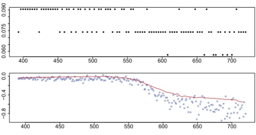
Figure 2.1: The bandwidth sequence (upper panel), plot of data and the estimated 90% quantile curve (lower panel)

literature considers structural semiparametric models to cope with curse of dimen- sionality, like, partial linear models, H¨ardle, Ritov & Song (2012), etc., additive models, Kong, Linton & Xia (2010), Horowitz & Lee (2005), etc; single index mod- els, Wu, Yu & Yu (2010), Koenker (2010), etc. Yet another strand of literature has been involved in ultra-high dimensional situations where a careful variable selection technique needs to be implemented, Belloni & Chernozhukov (2010) and Koenker (2010). In most of the aforementioned papers on non and semiparametric quantile regression, a smoothing parameter selection is implicit, and it is mostly a consequence of theoretical assumptions like e.g. rates of convergence, but falls short in practical hints for real data applications. An important exception is the method for local nonparametric kernel smoothing by Yu & Jones (1998) and Cai

& Xu (2008). They both propose a data driven choice of tuning parameter.

To address the limitations of the above mentioned literature on local model selec- tion for nonparametric quantile regression, we aim at proposing with theoretical justification an adaptive local quantile regression algorithm that is easy to imple- ment and works for a wide class of applications. The idea of this algorithm is to select tuning parameters locally by a sequence of likelihood ratio tests. The nov- elty lies in a local model selection technique with computable risk bounds. The main message is that the proposed algorithm is feasible and beneficial for quantile smoothing and helps in proposing alternatives to other models. As an example,

Ruppert, Wand & Carroll (2003). The presented quantile curve switches smooth- ness in the middle, and it is naturally reflected by the bandwidth sequence (upper panel) selected. In the presence of changing to sharper slope of the curve, the bandwidths get smaller to attain better approximations. This example shows that the paper algorithm can adaptively choose the bandwidth at each design point.

This article is organized as follows: In Section 2, we introduce the local model se- lection (LMS) procedure and lay down how to simulate critical values. In Section 3, Monte Carlo simulations are conducted to illustrate the proposed methodology. In Section 4, we apply our method on checking the tail dependency among portfo- lio stocks, and on estimation of quantile curves for temperature risk factors. In Section 5, we explain the main theorem on “Oracle” properties to support the validity of our tests, with the relevant assumptions, definitions and conditions in Appendix. In Section 6, we draw the conclusions. The technical details: 1, expo- nential risk bounds for conditional quantiles established using the representation of quantiles as Quasi Maximum Likelihood Estimation (qMLE)s of the asymmetric Laplace distribution, 2, theorems for the existence of critical values, 3, proof for

“propagation”, “stability” and “oracle” property are delegated to the Appendix.

2.2 Adaptive estimation procedure

This section introduces the considered problem and offers an adaptive estimation procedure.

2.2.1 Quantile regression model

Given the quantile level τ ∈ (0,1) , the quantile regression model describes the following relation between the response Y and the regressor X:

IP(Y > f(x)|X =x) = τ,

where f(x) is the unknown quantile regression function. This function is the target of the analysis and it has to be estimated from independent observations {Xi, Yi}ⁿi=1. This relation can also be represented as

Yi =f(Xi) +εi, (2.1)

where the errors εi follow IP(εi >0|Xi) = τ.

For simplicity of presentation, we consider a univariate regressor X ∈ IR¹ in this paper, an extension to the d-dimensional case X ∈ IR^d with d > 1 is straightforward.

2.2.2 A qMLE View on Quantile Estimation

The quantile function f(·) in (2.1) is usually recovered by minimizing the sum

n

X

i=1

ρτ{Yi−f(Xi) , (2.2)

over the class of all considered quantile functions f(·) , where ρτ(u)^def= u{τ1I(u≥ 0)−(1−τ) 1I(u <0)}. Such an approach is reasonable because the true quantile function f(x) minimizes the expected value of the sum in (2.2). An important special case is given by τ = 1/2 . Then an estimate of f(·) is built as minimizer of the least absolute deviations (LAD) contrast P

|Yi−f(Xi)|.

The minimum contrast approach based on minimization of (2.2) can also be put in a quasi maximum likelihood framework. Assume that the residuals εi are (2.1) be i.i.d. and π(x) is their negative log-density on IR¹. Then the joint log-density is given by the sum

−X

π Y_i−f(X_i)

and its maximization is equivalent to minimization of the contrast (2.2) with a special density function coming from the asymmetric Laplace distribution (ALD):

π(u) = πτ(u) = log

τ(1−τ) −ρτ(u), −∞< u <∞. (2.3) The parametric approach (PA) additionally assumes that the quantile regression function f(·) belongs to a parametric family of functions

fθ(x), θ∈Θ , where Θ is a subset of the p-dimensional Euclidean space. Equivalently,

f(x) = fθ^∗(x),

where θ^∗ is the true parameter which is usually the target of estimation.

Examples are a constant model:

fθ^∗(x)≡θ0, with θ^∗ =θ0 or a linear model:

fθ^∗(x) =θ0+θ1x, with θ^∗ = (θ₀, θ₁)^>.

Denote by IPθ the parametric measure on the observation space which corre-

εi following the asymmetric Laplace distribution (2.3). Then the log-likelihood L(θ) = L(Y,θ) for IPθ can be written as

L(θ) ^def= log

τ(1−τ)

n

X

i=1

1−

n

X

i=1

ρ_τ{Y_i−fθ(X_i)} (2.4) and the qMLE θe maximizes L(θ) , or, equivalently minimizes the contrast Pn

i=1ρτ{Yi− fθ(X_i)} over all θ∈Θ.

The described parametric construction is based on two assumptions: one is about the error distribution (2.3) and the other one is about the shape of the regression function f. However, it is only used for motivating our approach. Our theoretical study will be done under the true data distribution which follows mild regularity conditions. The next section explains how a smooth regression function f can be modeled by a flexible local parametric assumption.

2.2.3 Local polynomial qMLE

The global PA f(·) ≡fθ^∗(·) can be too restrictive in many applications. In what follows, we consider the local approach. Let a point x be fixed. The local PA at a point x ∈ IR only requires that the quantile regression function f(·) can be approximated by a parametric function fθ(·) from the given family in a vicinity of x. Below we fix a family of polynomial functions of degree p leading to the usual Taylor approximation:

f(u)≈fθ

def= θ0+θ1(u−x) +. . .+θp(u−x)^p/p! (2.5) for θ= (θ0, . . . , θp)^>. The corresponding parametric model can be written as

Yi =Ψ_i^>θ+εi, (2.6)

where Ψi ={1,(Xi−x),(Xi−x)²/2!, . . . ,(Xi−x)^p/p!}^> ∈IR^p+1.

A local likelihood approach at x is specified by a localizing scheme W given by a collection of weights wi for i = 1, . . . , n. The weights wi vanish for points Xi lying outside a vicinity of the point x. A standard proposal for choosing the weights W is wi = Kloc{(Xi−x)/h}, where Kloc(·) is a kernel function with a compact support, while h is a bandwidth controlling the degree of localization.

Define now the local log-likelihood at x by L(W,θ)^def= logτ(1−τ)

n

X

i=1

w_i −

n

X

i=1

ρ_τ(Y_i−Ψ_i^>θ)w_i.

This expression is similar to the global log-likelihood in (2.4), but each summand in L(W,θ) is multiplied with the weight wi, so only the points from the local vicinity of x contribute to L(W,θ) . Note that this local log-likelihood depends on the central point x via the structure of the basis vectors Ψi and via the weights wi. The corresponding local qMLE at x is defined via maximization of L(W,θ) : θ(x) =e {θe0(x),θe1(x), . . . ,θep(x)}^> (2.7)

def= argmax

θ∈Θ

L(W,θ)

= argmin

θ∈Θ

X

i=1

ρτ(Yi−Ψ_i^>θ)wi.

The first component θe0(x) provides an estimator of f(x) , while θem(x) is an estimator of the derivative f^(m)(x) , m= 1, . . . , p.

2.2.4 Selection of a Pointwise Bandwidth

The choice of bandwidth h is an important issue in implementing (2.7). One can reduce the variance of the estimation by increasing the bandwidth, but at a price of possibly inducing more modeling bias measured by the accuracy of approximation in (2.5); see Figure 2.2.

A desirable choice of a bandwidth at a fixed point would strike a balance between the variance and the bias depending on the local shape of f(·) in the vicinity of x. Many approaches have been proposed along this line; see e.g. ??? However, their justification and implementation is based on some asymptotic arguments and require large samples. Here we propose a pointwise bandwidth selection technique based on finite sample theory.

Our basic setup of the algorithm is described as follows. First one fix a finite ordered set of possible bandwidths h1 < h2 < . . . < hK, where h1 is very small, while hK should be a global bandwidth of order of the design range. The band- width sequence can be taken geometrically increasing of the form hk =ab^k with fixed a > 0 , b > 1 , and n⁻¹ < ab^k < 1 for k = 1, . . . , K (A.2.). The to- tal number K of the candidate bandwidths is then at most logarithmic in the sample size n. This value enters in the oracle risk bound and the suggested choice ensures that the adaptive procedure is nearly efficient up to a log-factor in the estimation accuracy. Accordingly, the sequence of ordered weighting schemes W^(k) = (w^(k)₁ , w₂^(k), . . . , wn^(k))^> is defined via w_i^{(k) def}= Kloc{(x−Xi)/hk}. This leads

to a family of estimates eθ₁(x),eθ₂(x), . . . ,eθ_K(x) with θe_k(x) = argmax

θ

L(W^(k),θ) = argmin

θ∈Θ

X

i=1

ρτ(Yi−Ψ_i^>θ)w_i^(k). (2.8) The proposed selection procedure is similar in spirit to Lepski, Mammen & Spokoiny (1997).

If the underlying quantile regression function is smooth, one can expect a good quality of approximation (2.5) for a large bandwidth values among {hk}^Kk=1. More- over, if the approximation is good for one bandwidth, it will be also suitable for all smaller bandwidths. So, if we observe a significant difference between the estimate eθ_k(x) corresponding to the bandwidth hk and an estimate θe<sub>`</sub>(x) corresponding to a smaller bandwidth h`, this is an indication that the approximation (2.5) for the window size hk becomes too rough. This justifies the following procedure.

Start with the smallest bandwidth h1. For any k >1 , compute the local qMLE eθ_k(x) and check it whether it is consistent with all the previous estimates eθ<sub>`</sub>(x) for ` < k. If the consistency check is negative, the procedure terminates and select the latest accepted estimate.

The most important ingredient of the method is the consistency check. We follow the suggestion from Polzehl & Spokoiny (2006) and apply the localized likeli- hood ratio type test. More precisely, the local MLE θe<sub>`</sub>(x) maximizes the log- likelihood value L W<sup>(`)</sup>,θ

, and the maximal value given by sup_θL W^(`),θ

= L W<sup>(`)</sup>,eθ<sub>`</sub>(x)

is compared with the particular log-likelihood value L W^{(`)</sup>,eθ<sub>k</sub>(x) , where the estimator θe<sub>k</sub>(x) is obtained by maximizing the other local log-likelihood function L(W<sup>(k)</sup>,θ) . The difference L W<sup>(`)},eθ_`(x)

−L W^(`),θe_k(x)

is always non-negative. The check rejects eθ_k(x) if this difference is too large, that is, if it exceeds any specified critical value for any ` < k. Equivalently one can say that the test checks whether eθ<sub>k</sub>(x) belongs to the confidence sets E<sup>`</sup>(z) of θe_`(x) :

E^`(z)^def=

θ :L W<sup>(`)</sup>,θe<sub>`</sub>(x)

−L W^(`),θ

≤z .

A great advantage of the likelihood ratio test is that the critical value z can be selected universally. This is justified by the Wilks phenomenon: the likelihood ratio test statistics is nearly χ² and its asymptotic distribution depends only on the dimension of the parameter space. Unfortunately, these arguments do not apply for finite samples and under possible model misspecification and we offer later another way of fixing the critical values z which is based on the so called propagation condition. We also allow that the width of the confidence set E`(z) depends on the index `, that is, z =z_`. Our adaptation algorithm can be summarized as follows: At each step k, an estimator θb_k(x) is constructed based

1 2 3 k^* k^*1 T3

T1 T²

Tk 1

Tk

Stop

CS

Figure 2.2: Demonstration of the local adaptive algorithm.

on the first k estimators eθ₁(x), . . . ,θe_k(x) by the following rule:

• Start with bθ₁(x) = eθ₁(x) .

• For k ≥2 , θe_k(x) is accepted and θb_k(x)^def= eθ_k(x) , if θe_k−1(x) was accepted and

L W<sup>(`)</sup>,θe<sub>`</sub>(x)

−L W^(`),θe_k(x)

≤z<sub>`</sub>, ` = 1, . . . , k−1. (2.9)

• The adaptive estimator bθ(x) is the latest accepted estimator after all K steps.

We also denote by θb_k(x) is the latest accepted estimator after the first k steps.

A visualization of the procedure is presented in Figure 2.2. The critical values z_`’s are selected by an algorithm based on the propagation condition explained in the next section.

2.2.5 Parameter Tuning by Propagation Condition

The practical implementation requires to fix the critical values of z₁, . . . ,z_K−1. We apply thepropagation approach which is an extension of the proposal from?. The idea of the approach is to tune the parameter of the procedure for one artificial parametric situation. Later we show that such defined critical value work well in the general setup and provide a nearly efficient estimation quality.

Similarly to Spokoiny (2009), the presented method can be viewed as a multiple

theory by ensuring a prescribed performance under the null hypothesis. In our case, the null hypothesis corresponds to the pure parametric situation with f(·)≡fθ^∗(·) in the equation (2.1). Moreover, we fix some particular distribution of the errors εi, our specific choice is the asymmetric Laplace distribution with the quantile parameter τ. Below in this section we denote by IPθ^∗ the data distribution under these assumptions.

For this artificial data generating process, all the estimates eθ_k(x) should be con- sistent to each other and the procedure should not terminate at any intermediate step k < K. We call this effect as propagation: in the parametric situation, the degree of locality will be successfully increased until it reaches the largest scale.

The critical values are selected to ensure the desired propagation condition which effectively means a “no false alarm” property: the selected adaptive estimate co- incides in the most of cases with the estimate θe_K(x) corresponding to the largest bandwidth. The event

eθ_k(x) 6= bθ_k(x) for k ≤ K is associated with a false alarm and the corresponding loss can be measured by the difference

L W^(k),eθ_k(x),θb_k(x) def

= L W^(k),eθ_k(x)

−L W^(k),θb_k(x) .

The propagation condition postulates that the risk induced by such false alarms is smaller than the upper bound for the risk of the estimator θe_k(x) in the pure parametric situation:

IEθ^∗L^r W^(k),eθ_k(x),bθ_k(x)

≤αRr k = 2, . . . , K, (2.10) where it holds for all k ≤K and

IEθ^∗L^r W^(k),eθ_k(x),θ^∗

≤ Rr

Here α and r are two hyper-parameters. The role of α is similar to the signifi- cance level of a test, while r denotes the power of the loss function. It is worth mentioning that

IEθ^∗L^r W^(k),eθ_k(x),θb_k(x)

→IPθ^∗

θe_k(x)6=bθ_k(x) , r →0.

The critical values {z_k}^Kk=1⁻¹ enter implicitly in the propagation condition: if the false alarm event {eθ_k(x)6=bθ_k(x)} happens too often, it suggests that some of the critical values z₁, . . . ,z_k−1 are too small. Note that (2.10) relies on the artificial parametric model IPθ^∗ instead of the true model IP. The point θ^∗ here can be selected arbitrarily, e.g. θ^∗ = 0 . This fact relies on linear parametric structure of the model (2.6) and is justified by the following simple lemma.

Lemma 1. The distribution of L W^(k),eθ_k(x),θb_k(x)

and of L W^(k),eθ_k(x),θ^∗ under IPθ^∗ does not depend on θ^∗.

Proof. Under PA f(·)≡fθ^∗(·) , it holds Yi−f(Xi) = Yi−Ψ_i^>θ^∗ =εi and hence, L(W^(k),θ) = log{τ(1−τ)}

n

X

i=1

w_i^(k)+

n

X

i=1

ρτ εi−Ψ_i^>(θ−θ^∗) w_i^(k).

A simple inspection of this formula yields that the distribution of L(W^(k),θ) only depends on u=θ−θ^∗. In other words, we can use the free parameter u=θ−θ^∗ whatever θ^∗ is, e.g. θ^∗ ≡ 0 . The same argument applies to the difference L W^(k),eθ_k(x),eθ_`(x)

for ` < k. Moreover, L W^(k),eθ_k(x),bθ_k(x)

is a function of

L W^(k),eθ_k(x),eθ_{`</sub>(x) <sup>k</sup><sub>`=1}, so the distribution of L W^(k),eθ_k(x),bθ_k(x) does not depend on θ^∗.

A choice of critical values z₁, . . . ,z_K−1 can be implemented in the following way:

• Consider first only z₁ and fix z₂ =. . .=z_K−1 =∞, leading to the estimates bθ_k(z1, x) for k = 2, . . . , K. The value z₁ is selected as the minimal one for which

1 Rr

IEθ^∗L^r W^(k),eθ_k(x),bθ_k(z₁, x)

≤ α

K−1, k = 2, . . . , K. (2.11)

• With selected z₁, . . . ,z_k−1, set z_k+1 = . . . = z_K−1 = ∞. Any particular value of z_k would lead to the set of parameters z₁, . . . ,z_k,∞, . . . ,∞ and the family of estimates bθ_m(z1, . . . ,z_k, x) for m = k+ 1, . . . , K. Select the smallest z_k ensuring

1

R^rIEθ^∗L^r W^(m),eθ_m(x),bθ_m(z1,z₂, . . . ,z_k, x)

≤ kα

K−1 (2.12)

for all m =k+ 1, . . . , K.

Few remarks to the proposed algorithm.

a. A value z₁ ensuring (2.11) always exists because the choice z₁ =∞ yields bθ_k(z₁, x) = eθ_k(x) for all k≥2 .

b. The value L^r W^(m),eθ_m(x),bθ_m(z₁,z₂, . . . ,z_k, x)

from (2.12) only accumu- lates the losses associated with the false alarms at the first k steps of the procedure, since the other checks at further steps are always accepted be- cause the corresponding critical values z_k+1, . . .z_K−1 are set to infinity.

c. The accumulated risk bound _K^kα₋₁ grows at each step by α/(K−1) . This

d. The value z_k ensuring (2.12) always exists, because the choice z_k=∞ yields bθ_m(z1,z₂, . . . ,z_k, x) = bθ_m(z1,z₂, . . . ,z_k−1, x)

for all m≥k.

e. All the computed values depend on the considered linear parametric model, the sequence bandwidths hk and the quantile level τ. They also depend on the local point x via the basis vectors Ψi. However, under usual regularity conditions on the design X1, . . . , Xn, the dependency on x is rather minor.

Therefore, the adaptive estimation procedure can be repeated at different points without reiterating the step of selecting the critical values.

2.3 Simulations

First, we check the critical values at different quantile levels (τ = 0.05,0.5,0.75,0.95 ) and for different noise distributions, ( a) Laplace, b) normal and c) student t(3) distribution). Also, we study how does misidentification of noise distribution af- fects critical values.

Second, we compare the performance of our local bandwidth algorithm with two other bandwidth selection techniques. One proposal is from Yu & Jones (1998), in which they consider a rule of thumb bandwidth based on the assumption that the quantiles are parallel, and another comes from Cai & Xu (2008), where an approach based on a nonparametric version of the Akaike information criterion (AIC) is implemented.

2.3.1 Critical Values

Table 2.1 shows the critical values with several choices of α and r with τ = 0.75 ,

m= 10000 Monte Carlo samples, and an bandwidth sequence (8,14,19,25,30,36,41,52)∗ 0.001 scaled for the interval [0,1] . Critical values decrease when α increases, and

increase when r increases, and the last 3 bandwidths equal to 0 , which is natu- ral, as by increasing the bandwidth, the variance of estimator decreases, and the size of the confidence set follows.

The bandwidth sequence in Table 2.2 displays critical values for different τ, with α= 0.25 , r= 0.5 , m= 10000 Monte Carlo samples, a bandwidth sequence H₁ = (8,14,19,25,30,36,41,52)∗0.001 , and N(0,1) noise. Critical values are roughly of the same level with respect to different τ.

Table 2.1: Critical Values with different r and α α = 0.25, r = 0.5 6.123 2.333 0.987 3.678e-05 0.000 α = 0.5, r = 0.5 4.616 1.578 0.357 2.472e-05 0.000 α = 0.6, r = 0.5 3.203 0.679 0.025 0.006 7.278e-05 α = 0.25, r = 0.75 9.127 3.288 1.031 0.126 5.675e-05 α = 0.25, r = 1 12.75 4.280 1.224 1.095e-04 0.000

Table 2.2: Critical Values with Different τ τ = 0.05 6.464 2.204 0.620 3.345e-05 0.000 τ = 0.5 7.997 3.089 0.986 0.300e-05 0.000 τ = 0.75 9.203 3.910 1.106 0.123 7.254e-05 τ = 0.95 8.589 5.452 1.904 0.334 1.203e-05

Table 2.3 displays the critical values for three alternative bandwidth sequences, i.e.

H₂ = (8,16,25,36,49,63,79,99)∗0.001 , H₃ = (5,8,14,19,27,36,46,58)∗0.001 and

H₁ = (8,14,19,25,30,36,41,52)∗0.001 , with α= 0.25 , r= 0.5 , and τ = 0.85 . We see that critical values differ for different bandwidth sequences, α, r and τ, but they show the same patterns (finite and decreasing). This in fact guarantees that our algorithm works for difference choice of bandwidth sequences.

Table 2.3: Critical Values with Different Bandwidth Sequences H₁ 11.33 1.243 6.933e-05 0.000 0.000

H₂ 18.39 6.479 2.230 0.469 8.738e-05 H₃ 6.123 2.333 0.987 3.678e-05 0.000

We simulate from different data generating processes, namely the distribution of εi

(π(.)) does not necessarily coincide with the likelihood (ALD_τ) taken to simulate critical values. Table 2.4 presents critical values simulated under t(3) , N(01) and ALDτ. The critical values show the same trend with some differences, so we conclude that a misidentification of error distribution would not significantly contaminate the confidence sets.

In Table 2.5, critical values are shown in the same circumstances as in Table 2.4 for the local linear case. Since introducing one more variable (trend), critical values

Table 2.4: Critical Values with Different Noise Distributions N(0,1) 11.50 4.924 2.514 1.313 2.765e-05 ALDτ 14.05 6.554 3.304 1.443 5.879e-05 t(3) 15.42 8.707 2.370 0.342 3.898e-05 to tail functions stays the same.

Table 2.5: Critical Values with Different Noise Distributions in Local Linear Case N(0,1) 29.97 58.64 43.21 33.41 19.43 07.40

ALD(0.5) 45.28 74.51 66.43 50.42 31.42 13.50 t(3) 51.77 84.94 59.28 44.99 29.07 11.57

2.3.2 Comparison of Different Bandwidth Selection Tech- niques

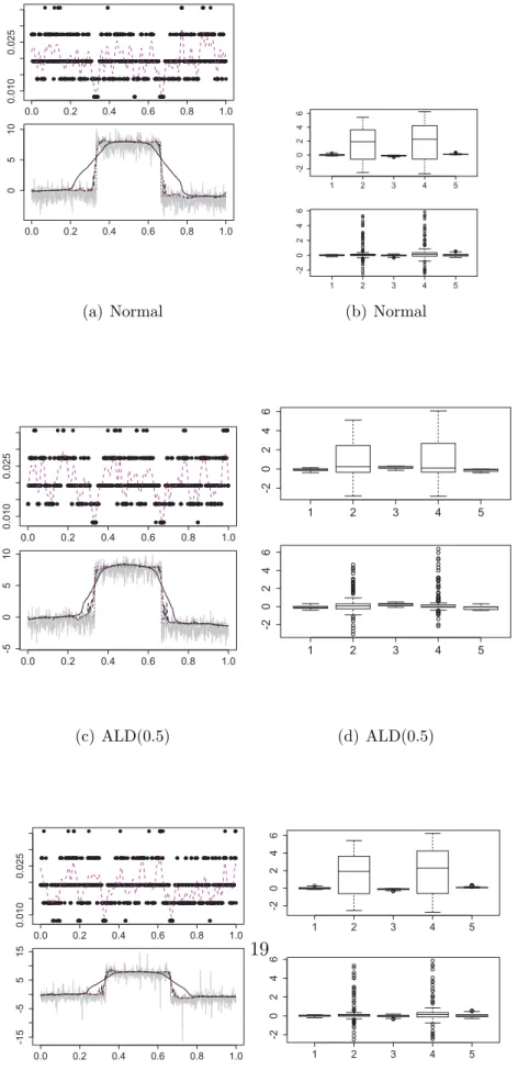
We illustrate our proposal by considering x ∈ [0,1] , τ = 0.75 . The sample with (n= 1000 ) are simulated under three scenarios:

f^[1](x) =







0 if x∈[0,0.333] ; 8 if x∈(0.333,0666] ;

−1 if x∈(0.666,1]

f^[2](x) = 2x(1 +x),

f^[3](x) = sin(k1x) + cos(k2x) 1I{x∈(0.333,0.666)}+ sin(k2x) The noise distributions are: N(0,0.03), ALDτ, t(3) .

Figure 2.3 presents pictures on comparisons of different estimates in the local constant case. Figure 2.4 and 2.5 show in the local linear case the estimators of the functions (f(x) ) and its first derivatives as well. Our technique providesb closer fits to the true curve (f(x) ) than methods with a global fixed bandwidth, especially in the presence of jump. Table 2.6, which shows the averaged absolute errors for the four methods, further confirms our conclusion.

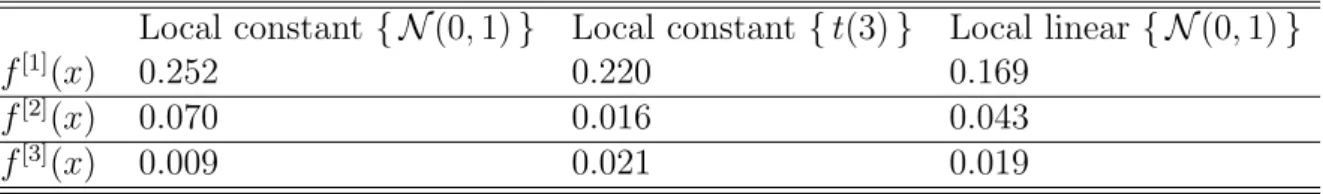
Table 2.7 offers further an analysis for misspecified error distributions. Specifi- cally, to evaluate the accuracy of our estimation for error distributions generated differently than the ALD density. Table 2.7 gives L1 errors between fb(·) (with critical values simulated from ALD_τ) and f(·) , from which we conclude that mis- specification of error distributions would not contaminate our results significantly.

0.0 0.2 0.4 0.6 0.8 1.0

0.0100.025

0.0 0.2 0.4 0.6 0.8 1.0

0510

(a) Normal

1 2 3 4 5

-20246

1 2 3 4 5

-20246

(b) Normal

0.0 0.2 0.4 0.6 0.8 1.0

0.0100.025

0.0 0.2 0.4 0.6 0.8 1.0

-50510

(c) ALD(0.5)

1 2 3 4 5

-20246

1 2 3 4 5

-20246

(d) ALD(0.5)

0.0 0.2 0.4 0.6 0.8 1.0

0.0100.025

0.0 0.2 0.4 0.6 0.8 1.0

-15-5515

(e) t(3)

1 2 3 4 5

-20246

1 2 3 4 5

-20246

(f) t(3)

Figure 2.3: The bandwidth sequence (upper left panel), the smoothed bandwidth (magenta dashed); the data with noise (grey, lower left panel), the adaptive esti- mation of 0.75 quantile (dashed black), the quantile smoother with fixed optimal

19

0.0 0.2 0.4 0.6 0.8 1.0

0.010.030.05

0.0 0.2 0.4 0.6 0.8 1.0

-100510

(a)

1 2 3 4 5

-10123

1 2 3 4 5

-1.00.0

(b)

Figure 2.4: The bandwidth sequence (upper left panel), the smoothed bandwidth sequence (dashed magenta); the observations (grey, lower left panel), the adaptive estimation of 0.75 quantile (dotted black), the true curve (solid black), the quan- tile smoother with fixed optimal bandwidth = 0.063 (dashed dotted blue), the estimation with adaptively smoothed bandwidth (dashed magenta); the blocked error of the adaptive estimator (lower right); the fixed estiamtor (upper right).

0 200 400 600 800 1000

-40-200204060

(a)

1 2 3 4 5

-60-40-20020

1 2 3 4 5

-60-40-20020

(b)

Figure 2.5: The adaptive estimation of first derivative of the above quantile func- tion (left panel grey), the true curve (solid black), the estimation with smoothed bandwidth (dashed black), the quantile smoother with fixed optimal bandwidth

= 0.045 (dotted black); the blocked error of the adaptive estimator (lower right);

the fixed estiamtor (upper right).

Table 2.6: Comparison of Monte Carlo errors, averaged over 1000 samples Fixed bandw Local constant Local linear Fixed bandw (Cai)

f^[1](x) 0.654 0.172 0.169 0.378

f^[2](x) 0.206 0.008 0.008 0.245

f^[3](x) 0.137 0.021 0.019 0.123

Table 2.7: Comparison of error mis-specification, errors are calculated averaged over 1000 samples

Local constant{ N(0,1)} Local constant{t(3)} Local linear { N(0,1)}

f^[1](x) 0.252 0.220 0.169

f^[2](x) 0.070 0.016 0.043

f^[3](x) 0.009 0.021 0.019

2.4 Applications

In the study of financial products, it is very important to detect and understand tail dependence among underlyings such as stocks. In particular, the tail depen- dence structure represents the degree of dependence in the corner of the lower-left quadrant or upper-right quadrant of a bivariate distribution. Hauksson, Michel, Thomas, Ulrich & Gennady (2001) and Embrechts & Straumann (1999) provide a good access to the literature on tail dependence and Value at Risk. With the adaptive quantile technique, we provide an alternative approach to study tail de- pendence.

The correlation is calibrated from real data as given in Figure 2.6, where X is standardized return from stock “clpholdings” from Hong Kong Hangseng Index, and Y is return from stock “cheung kong”. The conditional quantile function is linear, for example, X1 ∈ N(u1, σ1) and X2 ∈ N(u2, σ2) , the conditional quantile function α is:

f(x) =ϕ⁻¹(α)(σ2−σ₁₂² /σ1) +ui+σ12σ₂⁻¹(x−u2).

Figure 2.6 and Figure 2.7 show the empirical conditional quantile curves actu- ally deviate from the one calculated from normal distributions, which implies non normality. The motivation of adaptive bandwidth selection is clear to see from Figure 2.6 and Figure 2.7, the dependency structure change is more obvious com- pared with the fixed bandwidth curve. Moreover, the flexible adaptive curve is not likely to be a consequence of overfitting since it mostly lies in the confidence bands produced by fixed bandwidth estimation, see H¨ardle & Song (2010).