226 | Nature | Vol 577 | 9 January 2020
Long-term cyclic persistence in an experimental predator–prey system
Bernd Blasius1,2*, Lars Rudolf3, Guntram Weithoff4,5, Ursula Gaedke4,5 & Gregor F. Fussmann6
Predator–prey cycles rank among the most fundamental concepts in ecology, are predicted by the simplest ecological models and enable, theoretically, the indefinite persistence of predator and prey1–4. However, it remains an open question for how long cyclic dynamics can be self-sustained in real communities. Field observations have been restricted to a few cycle periods5–8 and experimental studies indicate that oscillations may be short-lived without external stabilizing factors9–19. Here we performed microcosm experiments with a planktonic predator–prey system and repeatedly observed oscillatory time series of unprecedented length that persisted for up to around 50 cycles or approximately 300 predator generations. The dominant type of dynamics was characterized by regular, coherent oscillations with a nearly constant predator–prey phase difference. Despite constant experimental conditions, we also observed shorter episodes of irregular, non-coherent oscillations without any significant phase relationship. However, the predator–prey system showed a strong tendency to return to the dominant dynamical regime with a defined phase
relationship. A mathematical model suggests that stochasticity is probably responsible for the reversible shift from coherent to non-coherent oscillations, a notion that was supported by experiments with external forcing by pulsed nutrient supply. Our findings empirically demonstrate the potential for infinite persistence of predator and prey populations in a cyclic dynamic regime that shows resilience in the presence of stochastic events.
Cyclic dynamics are one of the most notable phenomena in population biology and are known to occur in a large range of communities both in the wild5–8,13,14 and the laboratory9–12,15–18. A number of mechanisms that cause populations to oscillate have previously been identified3,4,20; the most highly investigated, however, are the cyclic dynamics that arise from trophic interactions between populations of predator and prey organ- isms. The nearly century-old fascination with this type of dynamics is rooted in the predictions of simple mathematical models, which suggest that the predator and prey may coexist on recurring cyclic trajectories over indefinitely long periods of time1,2. Empirical data that support the sustained nature of predator–prey cycles in the field are difficult to come by because tractable populations typically have cycle periods of three to ten years4,5,13. An alternative data source are laboratory studies with fast-reproducing organisms, with which long-running experiments can be realized under strictly controlled conditions9,10,12,16,21. In a seminal experimental study, population numbers of weevils and their larval parasites were recorded for a time span of about 20 cycles but oscilla- tions could not be sustained for the whole duration of the experiment10. This observation is paradigmatic for many studies, which showed that cycles in closed laboratory predator–prey systems tend to be short-lived, with populations either becoming extinct or reaching a stationary state.
These findings suggest that sustained, intrinsically generated preda- tor–prey cycles might be a construct of ecological theory and that
predator–prey systems require external drivers such as spatial struc- ture, immigration or environmental perturbations to exhibit persistent cycles9,11,12,17,22,23. To explore the potential for long-term persistence of predator–prey cycles, we cultured freshwater organisms—planktonic rotifers together with their prey, unicellular green algae—in several independent chemostat trials under constant environmental condi- tions (Methods, experiments C1–C7). One of our experimental systems (Fig. 1a and Extended Data Fig. 1; C1 in Extended Data Table 1) persisted without any external stimuli in a homogeneous environment for over a year and displayed more than 50 cycles, which is equivalent to about 300 predator generations and at least as many prey generations. This result of the long-term persistence of the predator and prey in a cyclic dynamic regime was confirmed in four additional, replicated chemostat experiments with the same species (C2–C5 in Extended Data Table 1, Extended Data Fig. 2), and in two additional experiments (C6 and C7) with a different algal prey species (Extended Data Fig. 3). We applied power analysis and phase analysis (in particular, bivariate wavelet analysis21,24–26) (Methods) to quantify the cyclic succession and the distribution of phase differences in our measured time series. Wavelet analysis revealed statistically significant associations between the dynamics of predator and prey densities in our experiments and power analysis determined a mean period length of 6.7 days (C1–C5) (Fig. 1d and Extended Data Fig. 1d, f).
https://doi.org/10.1038/s41586-019-1857-0 Received: 2 July 2019
Accepted: 18 November 2019 Published online: 18 December 2019
1Institute for Chemistry and Biology of the Marine Environment ICBM, University of Oldenburg, Oldenburg, Germany. 2Helmholtz Institute for Functional Marine Biodiversity, University of Oldenburg (HIFMB), Oldenburg, Germany. 3Institute of Physics and Astronomy, University of Potsdam, Potsdam, Germany. 4Department of Ecology & Ecosystem Modelling, University of Potsdam, Potsdam, Germany. 5Berlin-Brandenburg Institute for Advanced Biodiversity Research, Berlin, Germany. 6Department of Biology, McGill University, Montréal, Québec, Canada.
*e-mail: blasius@icbm.de
Nature | Vol 577 | 9 January 2020 | 227 Transitions between different oscillation regimes
Although the experiments were not perturbed by external influences, we identified sharp transitions between two different dynamic regimes.
For most of the time, we observed oscillations with a significantly coher- ent, nearly constant phase relationship (coherent oscillation regimes) (Methods), in which the predator densities followed the prey densities with a phase lag of about θ = 0.5π (equivalent to 90°), consistent with classical predator–prey theory. These periods with coherent oscilla- tions were intersected by non-coherent oscillation regimes in which the well-defined phase relationship between the measured signals was lost, but re-initiated shortly after (Fig. 1c, e). For example, the time interval between days 100 and 131 in C1 (Fig. 2a, b) and between days 37 and 66 in C7 (Fig. 2c, d) showed sustained cycles with regular period lengths and a constant phase lag between prey and predator densities, which is also reflected in the anticlockwise motion in the prey–predator phase plane (Fig. 1b). This regime of coherent oscillations gave way to a non- coherent, more irregular time series (days 132–161 in C1 and days 67–97 in C7), in which the phase relationship between prey and predator was lost, although both populations continued to oscillate (Fig. 2). Finally, and without external intervention, the system displayed resilience and the characteristic predator–prey phase difference was re-established.
Combining the analyses of all five experiments with the same preda- tor and prey species (C1–C5), we found that coherent oscillations were the dominant type of dynamics and comprised 66% of the total experi- mental time with a typical regime duration of 58 days (Extended Data Fig. 4 and Methods). In the remaining 34% of the experiments, predator and prey continued to oscillate, but without a well-defined phase rela- tionship (typical duration of non-coherent regimes, 23 days) (Methods).
Phase analysis of surrogate data revealed that spurious coherent oscil- lation regimes can arise also by chance, but with a significantly smaller duration (typical duration, 15 days) (Extended Data Fig. 4).
We performed additional analyses and experiments that were designed to provide mechanistic insights into the origin of the observed coherent oscillations and the intermittent breaks in the phase signature.
First, we extended the specificity of the phase analysis by including predator life-history stages. Second, we formulated and analysed a mathematical model that accounts for the predator’s stage structure.
And third, we performed three additional chemostat experiments: two experiments with periodic changes in the nutrient concentration in the supply medium, to explore how the phase relations were influenced by external forcing (C8 and C9); and one experiment at dilution rates that, according to bifurcation theory2,16 and our mathematical model, should cause the predator–prey system to cross over from oscillatory to equilibrium dynamics (C10).
Phase analysis of life-history stages
The predator in our system, the rotifer Brachionus calyciflorus27, is a small freshwater metazoan that reproduces asexually in the chemo- stats (only females occur) and undergoes a stage-structured life cycle.
Reproducing females carry 1–5 eggs, from which juveniles hatch and grow to adulthood without any larval stages; adults die shortly after the last egg has hatched. In addition to analysing algal and rotifer densi- ties, we applied phase analysis to all discernible predator life-history stages: the number of eggs, the egg ratio (that is, the average number of eggs per female rotifer) and the number of dead animals. We found that these life-history parameters also exhibited persistent cycles that were coherently locked in phase with prey abundance (Fig. 3a). These phase differences were notably constant over all different experimental replicates (Extended Data Figs. 1–3). Averaging across all experiments (C1–C5), we obtained the following phase signature: the predator den- sity followed the prey density with a phase difference of 93° ± 21°, the
a b
c d
e f
1.0
0.5
Abundance Predator
Time (days) Prey
0 50 100 150 200 250 300 350 0 1
1
0
0 1
2
16 8 4
Time (days) Power
0.5π
1.5π
π 0
0 50 100 150 200 250 300 350
Time (days)
0 50 100 150 200 250 300 350
Period length (days) Period length (days)
Phase difference (π)
0
2
8 4
16
1.5
0.5 1.0
0
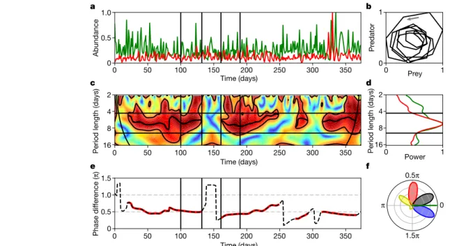
Fig. 1 | Phase analysis of a year-long, oscillatory predator–prey time series (experiment C1). a, Time series of the predator, B. calyciflorus (red) and its prey, Monoraphidium minutum (green); abundance normalized to a range of 0 to 1. b, Phase portrait of the bandpass-filtered predator–prey time series between days 90 and 135; the arrow indicates the direction of oscillation.
c, Wavelet coherence (WCO) between predator and prey. Values range from 0 (blue) to 1 (red). The cone of influence is indicated by black thin curved lines.
The black contour lines enclose significant areas (95% significance level, WCO > 0.83). The thick black line segments show the instantaneous oscillation
period ∼s t( ) of highest WCO within these areas (coherent oscillation regimes).
d, Global wavelet power spectrum P(s) for the predator (red) and the prey (green). e, Phase difference θ(t) between predator and prey; well-defined relations between both signals are marked in red. f, Circular distribution of the mutual phase difference to prey (indicated in green) for the predator (red), the predator egg ratio (blue), the number of eggs (black) and the dead animals (yellow). c, d, The two horizontal lines indicate the prefixed period band of [s1, s2]. a, c, e, The solid vertical lines indicate selected time spans of regular and irregular oscillations, which are enlarged in Fig. 2.
228 | Nature | Vol 577 | 9 January 2020
abundance of eggs was delayed to the abundance of prey with a phase difference of 27° ± 19°, whereas the egg ratio preceded the prey signal (−27° ± 16°); dead animals had a phase difference of −160° ± 68°. These mutual phase differences can be compactly visualized in a single cir- cular histogram21 (Figs. 1f and 3b). This ‘phase signature’ enables the straightforward interpretation of the temporal succession of the com- munity during the cycles and thus provides a fingerprint for the cyclic community structure.
Mathematical model
We compared our experimental results with numerical simulations of a stage-structured predator–prey model that included the operative parameters of the chemostat (inflow nutrient concentration and dilu- tion rate) and essential organismal variables (algae as well as rotifer eggs, juveniles, adults and dead animals) (Extended Data Fig. 5 and Methods). Numerical simulations revealed sustained oscillations with a period length of 6.8 days (experimental mean, 6.7 days). When we introduced stochasticity into the model, we observed similar breaks in the oscillation regimes as in experiments C1–C7, with random tran- sitions between coherent and non-coherent oscillating regimes that were triggered by stochasticity alone. We were still able to recover a phase signature that aligned well with the experimental observations (predator, 90° ± 11°; eggs, 11° ± 13°; egg ratio, −21° ± 2°; dead rotifers,
−150° ± 60°) (Fig. 3c, d and Extended Data Fig. 5).
Notably, both in the data and the model, the predator egg ratio pre- ceded the phase of prey availability, which is not immediately obvious as
egg production is directly connected to food availability. This phase lag between prey density and egg ratio disappeared in model simulations when the juvenile maturation rate was set to zero (Extended Data Fig. 6), revealing the effect of juveniles on the phase difference signature.
Juvenile predators (which, as immature individuals, carry no eggs by definition) have a crucial influence as they lead to an early breakdown of the egg-ratio maximum, caused by the multitude of non-egg-bearing juveniles during the prey maximum, finally giving rise to a negative phase difference between egg ratio and prey (Fig. 3a, c and Extended Data Fig. 6a). Thus, as physiological information may be encoded in the phase difference distributions, extending phase analysis to life-history stages enabled deeper insights into the functioning of our system.
Additional experiments
In experiments C8 and C9, we externally forced the dynamics through pulsed supply of nutrients (Methods). We chose a forcing period (8.0 days) that was clearly distinguishable from the period of the unforced experiments (6.7 days) but sufficiently close to enable, in theory, predator and prey (that is, living populations with demographic constraints) to lock to the external signal. Indeed, we observed predator–prey oscillations that were locked to the external signal, both in chemostat experiments and model results (Fig. 3e, g and Extended Data Fig. 7). As expected, oscillations were persistently coherent, without the non-coherent breaks in the time series from the unforced experiments (C1–C7), although intermittent period doubling occurred in experiment C8 (Fig. 3e and Extended Data a
b
c
d 1.2
0.4 0.8
Algae
0 2
8 4
Period length (days) 16
2
8 4
Period length (days) 16 8
2 6
Algae 4
0
100 125
25 75
50 Rotifers
0 20 60 40
Rotifers
0 Time (days)
100 110 120 130 140 150 160 170 180 190
Time (days)
100 110 120 130 140 150 160 170 180 190
Time (days)
40 50 60 70 80 90 100 110 120
Time (days)
40 50 60 70 80 90 100 110 120
Fig. 2 | Resilience of phase relationship in experiments with two different prey species. a, Enlarged view of the densities of the predator (animals per millilitre, red) and prey (M. minutum, 106 cells per millilitre, green) in experiment C1 for a time window of 90 days. b, Enlarged view of their WCO during the same time interval (colours and lines as in Fig. 1c). a, b, Solid vertical lines border a time interval without significant wavelet coherence between predator and prey, separating three dynamic regimes: days 100–131, distinct
predator–prey cycles with a constant phase shift of θ = π/2; days 132–161, regime of non-coherent oscillations (grey background); days 162–190, spontaneous re-initiation of the regular phase-locked oscillation. c, d, As in a, b, but showing a time window of 90 days for experiment C7 with a different algal prey, Chlorella vulgaris. Non-coherent oscillations arise between days 67 and 97.
Nature | Vol 577 | 9 January 2020 | 229 Fig. 7c, d). Notably, externally forced and unforced experiments
produced essentially the same phase signature (Fig. 3b, f), which was repeated also in model simulations (Fig. 3d, h). Thus, even in a dynamic regime that was strongly influenced by and locked to an external factor, phase analysis of different life-history stages was able to reveal the underlying predator–prey structure and to disen- tangle between intrinsic and external origins of cycles. This demon- strates that phase signature analysis can be a powerful diagnostic tool for the analysis of field data, for which it is often not known whether oscillations are the result of external factors or originate from species interactions.
Finally, we confirmed that the coherent oscillations observed in our experimental system indeed represent stable limit cycles, which arise from the destabilization of a stable equilibrium point. Oscilla- tions in experiment C10 persisted only in a certain parameter range;
if the dilution rate was increased, the oscillations died out (Extended Data Fig. 8). This result agrees with model predictions and previous experiments showing that increased dilution rates drive the system over a Hopf bifurcation16 (Extended Data Fig. 9).
Conclusions
Persistent and coherent predator–prey oscillations are a potential dynamic regime enabling the prolonged coexistence of predator and prey populations, as predicted by fundamental theory. In live systems, stochasticity and other external perturbations can obscure or prevent predator–prey oscillations, and our simulations suggest that stochas- ticity is probably responsible for the reversible shifts from coherent
to more-erratic oscillations that we observed in our highly controlled experiments. Four separate lines of evidence support a causal rela- tionship between sustained cycles and predator–prey interactions.
(1) Cyclic patterns dominated throughout the entire experiment and the system displayed resilience—that is, it returned to a well-defined phase relationship after intermittent non-coherent periods. (2) Planned experimental interventions enabled us to suppress cycles (C10) and to quench intermittent non-coherent oscillations (C8 and C9). (3) Data on the stage structure of the predator population enabled us to explicitly link characteristics of the predator–prey cycles to recurring changes in the demographic structure of the predator population. Therefore, our case for sustained predator–prey cycles is much stronger than it is pos- sible for unstructured microbial populations, in which population den- sities are the only variables. (4) Finally, the experimental predator–prey cycles manifested as a regular phase-locked succession, a pattern that we were able to capture as a community phase signature. Our approach firmly establishes this phase signature—which, in a similar way, can be constructed for any oscillating system—as a robust measure for identifying species interactions, cyclic or seasonal species succession, and the regulatory dependencies that underlie community dynamics.
Online content
Any methods, additional references, Nature Research reporting sum- maries, source data, extended data, supplementary information, acknowledgements, peer review information; details of author con- tributions and competing interests; and statements of data and code availability are available at https://doi.org/10.1038/s41586-019-1857-0.
0.5π
1.5π
π 0
0.5π
1.5π
π 0
0.5π
1.5π
π 0
0.5π
1.5π
π 0
Time (days)
AbundanceAbundanceAbundanceAbundance
10 15 20 25
a
c
e
g
b
d
f
h
30 35
Time (days)
0 5 10 15 20 25 30 35
Time (days)
45 50 55 60 65 70 75 80 85
Time (days)
0 5 10 15 20 25 30 35 40
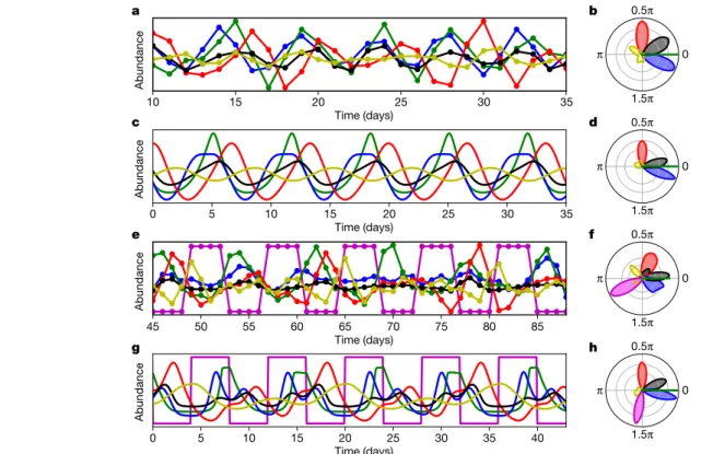
Fig. 3 | Dynamics and phase relationships in unforced versus externally forced systems. a, Time series of algae (green), rotifers (red), eggs (black), egg ratio (blue) and dead animals (yellow) in an unforced (that is, ‘free-running’
under constant conditions) experiment covering five oscillations (days 10–35 in C2). Data were filtered with a second order Butterworth bandpass filter and are shown in relative units. b, Phase signature aggregated over all experiments with the algal prey M. minutum under unforced conditions (C1–C5, including a total duration of 965 days), showing the circular distribution of the mutual phase differences to prey (colour code as in a). c, Simulated time series from
the predator–prey model under constant conditions with all stochasticity removed (mean centred, relative units). d, Phase signature obtained from stochastic simulations of the predator–prey model reproduces the
experimentally observed phase relationships and variances in b. e, As in a, but for an experiment with external forcing (days 45–88 of C8). The concentration of the external medium is shown in magenta. f, Phase signature aggregated over all experiments with external forcing (C8–C9, including a total duration of 323 days). g, h, As in c, d, but for simulations in an externally forced system.
230 | Nature | Vol 577 | 9 January 2020
1. Volterra, V. Fluctuations in the abundance of a species considered mathematically.
Nature 118, 558–560 (1926).
2. May, R. M. Limit cycles in predator–prey communities. Science 177, 900–902 (1972).
3. Kendall, B. E. et al. Why do populations cycle? A synthesis of statistical and mechanistic modeling approaches. Ecology 80, 1789–1805 (1999).
4. Berryman, A. A. (ed.) Population Cycles: The Case for Trophic Interactions (Oxford Univ.
Press, 2002).
5. Elton, C. & Nicholson, M. The ten-year cycle in numbers of the lynx in Canada. J. Anim.
Ecol. 11, 215–244 (1942).
6. Blasius, B., Huppert, A. & Stone, L. Complex dynamics and phase synchronization in spatially extended ecological systems. Nature 399, 354–359 (1999).
7. Gilg, O., Hanski, I. & Sittler, B. Cyclic dynamics in a simple vertebrate predator–prey community. Science 302, 866–868 (2003).
8. Ryabov, A. B., de Roos, A. M., Meyer, B., Kawaguchi, S. & Blasius, B. Competition-induced starvation drives large-scale population cycles in Antarctic krill. Nat. Ecol. Evol. 1, 0177 (2017).
9. Gause, G. F., Smaragdova, N. P. & Witt, A. A. Further studies of interaction between predators and prey. J. Anim. Ecol. 5, 1–18 (1936).
10. Utida, S. Cyclic fluctuations of population density intrinsic to the host–parasite system.
Ecology 38, 442–449 (1957).
11. Huffaker, C. B. Experimental studies on predation: dispersion factors and predator–prey oscillations. Hilgardia 27, 343–383 (1958).
12. Luckinbill, L. S. Coexistence in laboratory populations of Paramecium aurelia and its predator Didinium nasutum. Ecology 54, 1320–1327 (1973).
13. Krebs, C. J. et al. Impact of food and predation on the snowshoe hare cycle. Science 269, 1112–1115 (1995).
14. Hudson, P. J., Dobson, A. P. & Newborn, D. Prevention of population cycles by parasite removal. Science 282, 2256–2258 (1998).
15. McCauley, E., Nisbet, R. M., Murdoch, W. W., de Roos, A. M. & Gurney, W. S. C. Large- amplitude cycles of Daphnia and its algal prey in enriched environments. Nature 402, 653–656 (1999).
16. Fussmann, G. F., Ellner, S. P., Shertzer, K. W. & Hairston, N. G. Jr. Crossing the Hopf bifurcation in a live predator–prey system. Science 290, 1358–1360 (2000).
17. Ellner, S. P. et al. Habitat structure and population persistence in an experimental community. Nature 412, 538–543 (2001).
18. Becks, L., Hilker, F. M., Malchow, H., Jürgens, K. & Arndt, H. Experimental demonstration of chaos in a microbial food web. Nature 435, 1226–1229 (2005).
19. Massie, T. M., Blasius, B., Weithoff, G., Gaedke, U. & Fussmann, G. F. Cycles, phase synchronization, and entrainment in single-species phytoplankton populations. Proc.
Natl Acad. Sci. USA 107, 4236–4241 (2010).
20. Radchuk, V., Ims, R. A. & Andreassen, H. P. From individuals to population cycles: the role of extrinsic and intrinsic factors in rodent populations. Ecology 97, 720–732 (2016).
21. Benincà, E., Jöhnk, K. D., Heerkloss, R. & Huisman, J. Coupled predator–prey oscillations in a chaotic food web. Ecol. Lett. 12, 1367–1378 (2009).
22. Holyoak, M. & Lawler, S. P. Persistence of an extinction-prone predator–prey interaction through metapopulation dynamics. Ecology 77, 1867–1879 (1996).
23. Stenseth, N. C. et al. The effect of climatic forcing on population synchrony and genetic structuring of the Canadian lynx. Proc. Natl Acad. Sci. USA 101, 6056–6061 (2004).
24. Torrence, C. & Compo, G. P. A practical guide to wavelet analysis. Bull. Am. Meteorol. Soc.
79, 61–78 (1998).
25. Cazelles, B. et al. Wavelet analysis of ecological time series. Oecologia 156, 287–304 (2008).
26. Keitt, T. H. Coherent ecological dynamics induced by large-scale disturbance. Nature 454, 331–334 (2008).
27. Paraskevopoulou, S., Tiedemann, R. & Weithoff, G. Differential response to heat stress among evolutionary lineages of an aquatic invertebrate species complex. Biol. Lett. 14, 20180498 (2018).
28. Guillard, R. R. L. & Lorenzen, C. J. Yellow-green algae with chlorophyllide c. J. Phycol. 8, 10–14 (1972).
Publisher’s note Springer Nature remains neutral with regard to jurisdictional claims in published maps and institutional affiliations.
© The Author(s), under exclusive licence to Springer Nature Limited 2019
Methods
Data reporting
No statistical methods were used to predetermine sample size. The experiments were not randomized and the investigators were not blinded to allocation during experiments and outcome assessment.
Experiments
We ran chemostat experiments with parthenogenetic rotifers (B.
calyciflorus sensu strictu27, a small metazoan freshwater zooplankton species) as predators and unicellular algae (M. minutum or C. vulgaris) as prey under constant temperature (23 °C) and permanent illumina- tion. Experiments were conducted (mostly consecutively) in the same well-maintained climate chamber. We carefully searched for possible sources of external perturbations, but all measured parameters (for example, temperature and irradiance) remained constant throughout the experimental runs. For inoculation, we used stock cultures origi- nally raised from a single individual and added B. calyciflorus 10 days after the algae had reached a biomass that enabled rotifer growth. The chemostats (experimental volume, 0.8 l) had a constant inflow of sterile medium with a rate of 0.55 per day. We used a modified WC medium28 with a reduced nitrogen concentration of 80 μmol l−1 nitrate as the limiting resource. In the experiments with external forcing, we periodi- cally changed the concentration in the external medium to between 0 and 160 μmol l−1 nitrate with a period length of 8 days. We took daily subsamples of 8 ml to determine the abundance of both predator and prey. The algal abundance was analysed with an electronic particle counter (CASY, Schärfe). The rotifers were counted using an inverted microscope at 100-fold magnification. For the rotifers, we recorded the total number of rotifers and of asexually produced subitaneous eggs and the dead animals. No males or sexually reproducing females were observed throughout the experiment. The egg ratio (that is, the total number of eggs divided by the total number of animals in the population) is a measure of the reproductive status of the population.
Bivariate wavelet analysis
Because the measured signals showed large variability, we applied phase analysis6, which relies on the fact that the regulatory depend- ence between state variables is often encoded in their phase relation- ship, whereas the amplitudes may be highly erratic and uncorrelated6. The wavelet method24 is a particularly powerful tool for extracting optimally resolved phase information from ecological time series25,26 and enables us to quantify transient associations between two non- stationary signals24,29–32.
Continuous wavelet transformation
The continuous wavelet transformation24 (CWT) of a signal x(t) is calculated as the convolution of the signal with a localized complex- valued wavelet function ψ(τ) centred at time t and dilated by the scale parameter s
∫
W s t
s t x t ψ t t ( , ) = 1 d ′ ( ′) ′ −s
x ⁎
Here, the asterisk denotes the complex conjugate. After decompos- ing the complex CWT into amplitude and phase W s tx( , ) = W s tx( , ) eiϕ s tx( , ) intuitively it can be understood as the extent W s tx( , ) to which the signal x(t) at local time t resembles an oscillation with period length s and phase ϕx(s, t).
Throughout our analysis, we used the Morlet wavelet ψ τ( )=
π−1/4eiω τ0e− /2τ2 with ω0 = 6 so that the scale parameter s can simply be interpreted as the period length of the oscillation24. We always took s from 100 uniform steps per octave on a logarithmic scale. Edge effects were minimized by applying zero padding to the time series to the next
highest integer power of two. We always indicate the cone of influence, which marks the zone in the CWT that is affected by edge effects24. Wavelet power spectrum
Although the wavelet transform is complex, the real-valued local wavelet power spectrum (WPS) of a signal x(t) at time t and scale s can be defined as
W s txx( , ) = W s t W s tx( , ) x⁎( , )
in which ‘⟨…⟩’ denotes a smoothing operator in both scale and time (see
‘Parametrization and smoothing’). The global WPS Px(s) is defined as the time average of the local WPS and measures the averaged variance of the signal x(t) at scale s. We used the maximum of Px(s) to estimate the mean oscillation period of the signal.
Wavelet cross-spectrum
To quantify the statistical relationship between two non-stationary signals x(t) and y(t), the wavelet cross-spectrum (WCS) is defined as the smoothed product of the corresponding wavelet transforms24,29–31
Wx y,( , ) =s t W s t W s tx( , ) ⁎y( , )
The WCS is complex-valued. After decomposition into amplitude and phase Wx y,( , ) =s t Ax y, ( , ) es t i ϕΔ x y, ( , )s t, the phase describes the de-lay
ϕ s t ϕ s t ϕ s t
Δ x y, ( , ) = ( , ) − ( , )x y between the two signals at time t and scale s, whereas the amplitude Ax,y(s, t) expresses the covarying power of the two processes.
Wavelet coherence
The WCS is not specific, because it exhibits high values when either a true covariance between the two signals exists or when one of the spec- tra exhibits a high value. To solve this problem, a normalized measure is given by the WCO29–31, which is defined as the amplitude of the WCS divided by the square roots of the two local WPS
s t W s t
W s t W s t
WCO ( , ) = ( , )
( , ) ( , )
x y
x y
x x y y
,
,
, 1/2
, 1/2
The WCO estimates the relationship between the two signals at time t and scale s, normalized into the range 0 ≤ WCO ≤ 1. As the WCO is real- valued, it cannot be used to extract the delay between two signals, in contrast to the WCS.
Dominant phase difference
The phase difference Δϕx,y(s, t) between two signals x(t) and y(t), as obtained from the WCS, depends on the scale parameter s. Assume now that the two signals oscillate with a common, but possibly time- varying, period length. To obtain their dominant phase difference, we define for every time instance t the dominant scale s t∼( ) as the scale parameter that has the maximal WCO at time t over all scales in a pre- fixed band [s1, s2]:
∼s t( ) = argmaxs s s< < WCO( , )s t
1 2
These values∼s t( ) constitute a line of the strongest co-oscillating component of both signals in the timescale plane32. Inserting this line in the WCS yields the dominant phase difference θx,y(t) between the two signals at every time instance
∼ ∼
θx y,( ) =t ϕ s t tx( ( ), ) − ( ( ), )ϕ s t ty
Significance testing
To assess the statistical significance of the WCO, we generated n = 1,000 independent realizations of surrogate data by time-scrambling the
empirical signals (that is, sampling 1,000 random values with replace- ment from the measured predator and prey time series). The resulting surrogate data retain the frequency histogram of the original data but lose all temporal correlations. Using Monte Carlo simulations, we found that for our chosen parameterization (see ‘Parametrization and smoothing’) two signals are significantly correlated at time t and scale s on a 95% critical level if WCO(s, t) = 0.83.
Coherent oscillation regime
We defined a maximal contiguous time interval for which the dominant scales t∼( ) is within a statistically significant area in the timescale plane—
that is, being inside the cone of influence and having a significant
∼s t t
WCO( ( ), ) > 0.83—as a coherent oscillation regime. The remaining time intervals constitute the non-coherent oscillation regimes. Each signal on its own may well oscillate in a regular fashion even within a non-coherent oscillation regime, but for a pair of signals the wavelet analysis guarantees a significantly correlated oscillation—and therefore a well-defined phase relationship—only in a coherent oscillation regime.
To characterize the typical duration T of coherent oscillations in an ∼ ensemble of signals, we first measure the length Ti of each coherent oscillation regime i = 1 … N that occurs in the ensemble and then cal- culate the expected oscillation regime duration, T , of a randomly cho-∼ sen time instance taken from a coherent oscillation regime T∼= ∑iN=1Ti2/ ∑iN=1Ti. We found that this measure gives a better description of the typical time to observe a coherent oscillation inter- val than the median or the mean T= ∑iN=1T Ni/ of the length distribution.
Circular phase distribution
To characterize the phase relationship between a pair of covarying signals, we calculated the dominant phase differences θk for all time instances within a coherent oscillation regime. We used circular sta- tistics33 to characterize the resulting distribution of phase differences θk. For this we calculated the complex order parameter z, which is defined as the average of the complex numbers eiθk
∑
z R= e =N1
iθ e
k N iθ
=1 k
Here the phase angle θ of z indicates the circular mean of the phase differences, and the amplitude R of z gives the circular standard devi- ation of the distribution as −2 ln .R
Given the sampling frequency of 1 day−1, the Nyquist frequency is 0.5 day−1, which for an average period length of 6.7 days roughly cor- responds to a phase resolution of 27°. Averaging phase differences over many cycles enabled us to achieve a much better phase resolution, yielding typically rather smooth distributions of phase differences.
We verified that these smooth phase distributions are no artefacts, by comparing phase distributions obtained from our highly resolved numerical simulations (see ‘Numerical simulation’) with those obtained from time series sampled from these simulations once per day, which yielded very similar results.
Phase signature
To characterize the mutual phase relationship of not only two but also an ensemble of time series (for example, total densities of predator and prey and of measured life history stages), we calculated the distribution of phase differences of all time series with respect to one selected reference time series. The combined plot of all resulting circular distributions in one common polar histogram defines our ‘phase signature’, providing a fingerprint for the cyclic succession of the corresponding state variables.
Parametrization and smoothing
Following a previously published study31, we performed smoothing in time by convolution with a normalized real Morlet wavelet
τ s s
exp[− /(2 )]/( 2π )2 2 . Smoothing in scale direction was obtained by averaging over a constant-length (boxcar) window over 0.6 octaves—the scale decorrelation length for the Morlet wavelet—on a logarithmic scale31. Similarly, we took the upper and lower scale band borders s1
and s2 as ± 0.6 octaves from the peak in the global (that is, time-aver- aged) WCS. For a better visualization, circular histograms (bin width of π/100) were smoothed by a moving average (window width 0.15π, the above calculated phase resolution).
We verified that the resulting phase distributions remain largely unchanged for different parameterizations of the wavelet analysis, in particular for different wavelet functions, different values of the wavelet parameter ω0, different smoothing parameters and scale band borders s1 and s2.
Numerical simulation
We developed a mathematical model to describe a stage-structured predator–prey community in a chemostat34,35, which closely follows our experimental setup. The model includes as state variables the concentration of nitrogen N, phytoplankton P, and three life stages of the predator, namely eggs E, juveniles J and adults A. Additionally the model keeps track of the dead animals D in the chemostat. We assume a constant time delay θ for egg development, a constant time delay τ for juvenile maturation, and the same constant mor- tality rate for juveniles and adults (deliberately keeping the model simple, as intake-related regulations34,35 did not improve the agree- ment between simulation results and data). We assume that the phy- toplankton population is unstructured. All variables are measured in μmol N l−1.
The model is written as the following system of time-delayed ordinary differential equations:
̇̇̇̇̇̇
N δN F N P δN P F N P F P B ε δP E R R δE
J R R m δ J
A βR m δ A
D m J A δD
= − ( ) −
= ( ) − ( ) / −
= − −
= − − ( + )
= − ( + )
= ( + ) −
in P
P B
E J
J A
A
Here, β is the adult/juvenile mass ratio (the juvenile/egg mass ratio is assumed to be 1) and the recruitment rates are
R t F P t A t
R t R t θ δθ
R t R t τ δτ
( ) = ( ( )) ( ) ( ) = ( − ) exp(− )
( ) = ( − ) exp(− )
E B
J E
A J
Algal nutrient uptake FP(N) is modelled as a Monod function and predator recruitment as a type-3 functional response with Hill coef- ficient κ
F N r N
K N
F P r P
K P
( ) = + ( ) = +
κ
κ κ
P P
P
P B
B
The total predator density is given by B(t) = βJ(t) + A(t) and the egg ratio is βE(t)/B(t). As state variables are given in units of nitrogen, juve- niles and eggs here need to be scaled by the adult/juvenile mass ratio β.
The model is solved numerically by an Euler scheme with a time step of h = 0.001 days. We included environmental stochasticity by taking the growth rates rP and rB as autocorrelated random num- bers by multiplying them in every time step i with a factor of 1 + si.
Autocorrelation (that is, red noise) is implemented as si + 1 = asi + ξi (first-order autoregressive AR(1) process36) with autocorrelation parameter a and independent and identically distributed Gaussian numbers ξi with mean 0 and variance σ2(1 −a2). For wavelet analysis and for representation in figures, the simulated states are sampled with a rate of 1 per day, in accordance with the experiments. To cap- ture measurement error and additional stochastic influences, we replaced the sampled rotifer state variables, E(t), J(t), A(t) and D(t), by random values drawn from a Poisson distribution with an expecta- tion value equal to that of the state variable. Finally, algal and rotifer state variables were rescaled to individuals per volume using the constants νP, and νB, respectively.
Parameter values were taken as follows. Mass ratio adult/juve- niles, β = 5; dilution rate, δ = 0.55 per day; nitrogen concentration in the external medium, Nin = 80 μmol l−1; phytoplankton maximal growth rate, rP = 3.3 per day; phytoplankton half-saturation constant:
kP = 4.3 μmol l−1; rotifer maximal egg-recruitment rate, rB = 2.25 per day; rotifer half-saturation constant, kB = 15 μmol l−1; Hill coefficient of the functional response, κ = 1.25; predator assimilation efficiency, ε = 0.25; rotifer mortality rate, m = 0.15 per day; egg development time, θ = 0.6 days; juvenile maturation time, τ = 1.8 days; autocorrelation parameter, a = 0.9; noise strength, σ = 0.5; nitrogen content per adult female Brachionus, νA = 0.57 × 10⁻³ μmol N per female; nitrogen content per algal cell, νP = 28 × 10−9 μmol N per cell.
Environmental parameters (δ, Nin) were taken according to the experimental set-up. Parameters for uptake and growth (rP, kP, rB, kB
and ε) were taken according to a previous study16. The rotifer mortality rate (m) was increased compared with this previous study16, as we did not include the loss of the reproducing rotifer cohort into senescent animals. The mass ratio of adults to juveniles (β) was taken from the literature37. Duration of development stages (θ, τ) was adjusted to be within the previously reported range38. We used a type-3 functional response39,40. Only the parameter values of population dynamics (θ, τ, κ and m) and stochasticity (noise levels and noise colour) were adjusted by hand within ecologically reasonable ranges to simultane- ously optimally fit the comprehensive experimental data. As criteria we used the observed range and variability of the state variables, existence of oscillatory dynamics with correct period length, phase signatures (that is, phase relationships between all state variables, including the egg ratio), power and wavelet spectra, and the typical duration of coherent oscillatory regimes—both in the unforced and forced scenarios.
Reporting summary
Further information on research design is available in the Nature Research Reporting Summary linked to this article.
Data availability
Experimental data are publicly available on Figshare (https://doi.
org/10.6084/m9.figshare.10045976.v1).
Code availability
Data analysis and the model were implemented in the language Julia v.1.141. The source code for the wavelet analysis is publicly available on GitHub (https://github.com/berndblasius/WaveletAnalysis).
29. Torrence, C. & Webster, P. J. Interdecadal changes in the ENSO–monsoon system. J. Clim.
12, 2679–2690 (1999).
30. Maraun, D. & Kurths, J. Cross wavelet analysis: significance testing and pitfalls. Nonlin.
Processes Geophys. 11, 505–514 (2004).
31. Si, B. C. Spatial scaling analyses of soil physical properties: a review of spectral and wavelet methods. Vadose Zone J. 7, 547–562 (2008).
32. Bandrivskyy, A., Bernjak, A., McClintock, P. & Stefanovska, A. Wavelet phase coherence analysis: application to skin temperature and blood flow. Cardiovasc. Eng. 4, 89–93 (2004).
33. Batschelet, E. Circular Statistics in Biology (Academic, 1981).
34. McCauley, E., Nisbet, R. M., de Roos, A. M., Murdoch, W. W. & Gurney, W. S. C. Structured population models of herbivorous zooplankton. Ecol. Monogr. 66, 479–501 (1996).
35. de Roos, A. M. & Persson, L. Population and Community Ecology of Ontogenetic Development 59 (Princeton Univ. Press, 2013).
36. Massie, T. M., Weithoff, G., Kuckländer, N., Gaedke, U. & Blasius, B. Enhanced Moran effect by spatial variation in environmental autocorrelation. Nat. Commun. 6, 5993 (2015).
37. Mourelatos, S., Pourriot, R. & Rougier, C. Taux de filtration du rotifère Brachionus calyciflorus: comparaison des méthodes de mesure; influence de l’âge. Vie Milieu 40, 39–43 (1990).
38. Halbach, U. Einfluß der Temperatur auf die Populationsdynamik des planktischen Rädertieres Brachionus calyciflorus Pallas. Oecologia 4, 176–207 (1970).
39. Fussmann, G. E., Weithoff, G. & Yoshida, T. A direct, experimental test of resource vs.
consumer dependence. Ecology 86, 2924–2930 (2005).
40. Seifert, L. I. et al. Heated relations: temperature-mediated shifts in consumption across trophic levels. PLoS ONE 9, e95046 (2014).
41. Bezanson, J., Edelman, A., Karpinski, S. & Shah, V. B. Julia: a fresh approach to numerical computing. SIAM Rev. 59, 65–98 (2017).
Acknowledgements This work was supported by German VW-Stiftung. We thank A.
Bandrivskyy, T. Massie, E. Denzin and all other technical staff of the Department of Ecology &
Ecosystem Modelling; and R. Ceulemans, C. Feenders, A. Jamieson-Lane, A. Ryabov and E. van Velzen for comments on the manuscript.
Author contributions B.B., G.F.F., G.W. and U.G. designed the research, L.R., G.F.F. and G.W.
performed the experiments, B.B. and L.R. performed the numerical simulations and data analysis, B.B. and G.F.F. wrote the paper. All authors discussed the results and commented on the manuscript.
Competing interests The authors declare no competing interests.
Additional information
Supplementary information is available for this paper at https://doi.org/10.1038/s41586-019- 1857-0.
Correspondence and requests for materials should be addressed to B.B.
Peer review information Nature thanks Alan Hastings and the other, anonymous, reviewer(s) for their contribution to the peer review of this work.
Reprints and permissions information is available at http://www.nature.com/reprints.
Extended Data Fig. 1 | Detailed dynamics and phase relationship in experiment C1. a, Time series of the predator, B. calyciflorus (red), and its prey, M. minutum (green), (normalized to the range of 0 and 1). b, Phase portrait of the bandpass-filtered predator–prey time series between days 90 and 130. The arrow indicates the direction of oscillation. c, Local WPS for the prey, ranging from 0 (blue) to maximum (red), and the instantaneous oscillation period ∼s t( ) (black line) of the highest WCO within the prefixed period length band (horizontal black lines). The cone of influence is also indicated (black).
d, Global WPS P(s) for the prey (green). Horizontal lines as in c. e, f, As in c, d, but for the predator. g, WCS between predator and prey, colour-coding and other lines as in c. h, Amplitude of the global WCS for the predator and the prey.
i, WCO between predator and prey, ranging from 0 (blue) to 1 (red). Significant areas (WCO > 0.83) are enclosed by thin solid lines; the thick black line segments show the instantaneous oscillation period ∼s t( ) in these segments.
j, Histogram of period lengths within coherent oscillation regions as detected in i. k, Phase difference θ(t) to prey for the predator (red), the predator egg ratio (blue), the number of eggs (black) and dead animals (yellow). Significant relations between respective signals are marked as a solid line. l, Circular distribution of the mutual phase difference to prey (indicated in green) for the predator (red), the predator egg ratio (blue), the number of eggs (black) and dead animals (yellow).
Extended Data Fig. 2 | Dynamics and phase relationships in three further experimental time series in a constant environment. a–d, Analysis of experiment C2. a, Predator–prey time series. b, Phase signature. c, WCO. d,
Global WPS. e–h, As in a–d, for experiment C3. i–l, As in a–d, for experiment C4.
Details and colours as in Fig. 1.
Extended Data Fig. 3 | Dynamics and phase relationships in measured time series with a different algal species (C. vulgaris). a–d, Analysis of experiment C6. a, Predator–prey time series. b, Phase signature. c, WCO. d, Global WPS. e–h, As in a–d, for experiment C7. Details and colours as in Fig. 1.
Extended Data Fig. 4 | Dynamics and phase relationship in surrogate data and length distribution of coherent oscillation regimes. a–f, As in Fig. 1, but for surrogate data, obtained by time scrambling—that is, randomly drawing 360 values with replacement from the predator and prey time series in experiment C1—yielding a time series without temporal correlation (white noise) but with the same abundance distribution as the experimental data. The figure shows a typically outcome. Occasionally, for short bursts the
randomized predator and prey time series oscillate with a common frequency (a), yielding areas of high coherence (c; WCO > 0.83; spurious coherent oscillation regimes) with random phase differences (e). Whereas most time intervals with coherent predator–prey cycles in the surrogate data have a short duration, in this example (by chance) there is one regime (days 187–209) with a duration of 23 days. g, h, Box plots of oscillation regime length. Boxes show the interquartile range, orange lines indicate the median, whiskers range from the lowest to the highest data point within 1.5× the interquartile range and markers indicate outliers. g, Length distribution of coherent oscillation regimes for the
experimental data under free-running conditions (C1–C5) and for a large ensemble of surrogate data. This shows that time intervals with coherent oscillations are significantly longer in the experiments (n = 20; median, 16 days;
mean ± s.d., 29 ±28 days) than in the surrogate data (n = 13,719; median, 8 days;
mean ± s.d., 9 ± 7 days). The two outliers in the left box plot correspond to the two long coherent oscillation regimes of 111 days and 85 days in C1, which (even though they are outliers in the length distribution) effectively dominate the dynamic behaviour in C1. Consequently, we calculate the typical duration T of ∼ coherent oscillations as the expected regime duration for a randomly chosen time instance taken from a coherent oscillation regime (Methods) (T = 58 days ∼ in C1–C5; T = 15 days in the surrogate data). h, As in g, but for durations of non-∼ coherent oscillation regimes, showing that time intervals of non-coherent oscillations are significantly shorter in the experiments (n = 15; median, 17 days;
mean ± s.d., 16 ± 11 days; typical duration T = 23 days) than in the surrogate data ∼ (n = 12,719; median, 43 days, mean ± s.d., 60 ± 11 days; typical duration T = 113 days).∼
Extended Data Fig. 5 | Detailed dynamics and phase relationships in a modelled time series. a–l, As in Extended Data Fig. 1, but for a simulated time series of the stochastic time-delayed model in a constant environment. The simulation time was 300 days. A typical model outcome is shown. In this
example, we obtained five coherent oscillation regimes (indicated as thick lines in i, k). Similar to the experimental systems (C1–C7), these regimes are interspersed by short non-coherent oscillation regimes without a significant phase relationship.
Extended Data Fig. 6 | Dynamics and phase relationships in a model without juvenile maturation delay. a, Simulated time series of algae (green), rotifers (red), eggs (black), egg ratio (blue) and dead animals (yellow) in a model without juvenile maturation delay, τ = 0, under constant conditions with all stochasticity removed (mean centred, relative units). b, Phase signature obtained from stochastic simulations (free-running conditions, τ = 0). c, d, As in a, b, but for an externally driven system (external nutrient concentration shown in magenta). The figure shows that in a scenario without juvenile maturation delay (τ = 0), the phase of the egg ratio coincides with that of the
algae, both in a free-running and in an externally driven model. This is in contrast to the experimental observations (Fig. 3, rows 1 and 3) and simulations with non-vanishing juvenile maturation delay (τ = 1.8 days) (Fig. 3 rows 2 and 4, Extended Data Fig. 9d, f), in which the egg ratio is significantly preceding the algae signal. Thus, the phase signature helps to disentangle life-history mechanisms, as—by comparison of observed and simulated phase signatures—a delay of juvenile maturation is essential to attain the experimentally observed phase relations.
Extended Data Fig. 7 | Dynamics and phase relationships in externally driven systems. a–d, Analysis of experiment C8. a, Predator–prey time series. b, Phase signature. c, WCO. d, Global WPS. e–h, As in a–d, for experiment C9. i–l, As in a–d, for simulation results of an externally driven system. Details and colours
as in Fig. 1. In a, e, i, the blue dotted line shows the input concentration in the external medium in normalized units. In b, f, j, the phase difference distribution between the external medium and the prey is shown in magenta.
Extended Data Fig. 8 | Dynamics and phase relationships in experiments and simulations with changed dilution rate and press perturbations. a–d, Analysis of experiment C5, which has an increased dilution rate (δ = 0.66 per day). a, Predator–prey time series. b, Phase signature. c, WCO. d, Global WPS.
e–h, As in a–d, for experiment C10, which undergoes press perturbations (vertical black lines) at day 84 (dilution rate was increased from δ = 0.55 per day
to δ = 1.2 per day) and day 123 (dilution rate increased further to δ = 1.35 per day). i–l, As in a–d, with simulation results of a system undergoing a press perturbation in which the dilution rate was increased to δ = 0.75 per day at day 100 (vertical black line in i, k). Under conditions of the increased dilution rate, the oscillations are suppressed (Extended Data Fig. 9a). Details and colours as in Fig. 1.
Extended Data Fig. 9 | Bifurcation diagrams. a, Simulated values of predator (red) and prey (green) for different values of the dilution rate. Thick solid lines show maximal and minimal values obtained in the unforced model without stochasticity. Shaded areas show range of values in the stochastic model.
Sustained predator–prey oscillations appear for 0.47 < δ < 0.71 per day. For large values of the dilution rate, δ > 0.87 per day, the predator goes extinct. b, As in a, but for the externally forced system. The model shows oscillations for all parameters without predator extinction δ < 0.8 per day, it exhibits a bistability regime (small- versus large-amplitude oscillations) for
0.23 < δ < 0.31 per day and a period-2 oscillation regime for 0.42 < δ < 0.57 per day. c, d, Bifurcation diagrams of the unforced model as a function of the
juvenile maturation delay τ. c, As in a, but for the different bifurcation parameter. d, Phase difference to the algae for the predator (red), eggs (black) and the egg ratio (blue). The shaded areas indicate the range of phase differences (±1 s.d.) from the experiments in a constant environment (C1–C5).
For large values of τ, the simulated phase signature aligns with the experimental data, whereas for small values of τ, the simulated phase difference of the egg ratio approaches zero. e, f, As in c, d, but for the externally forced model. e, For small delay times, 0.4 < τ < 1 day, the model exhibits a chaotic regime. f, Additionally the phase difference between algae and external nutrients is shown (magenta). Vertical solid lines show the actually used parameter values δ = 0.55 per day and τ = 1.8 days.
Extended Data Table 1 | Summary of all experiments
N
i( )
A series of ten chemostat experiments was performed, constituting a total of 1,948 measurement days (corresponding to 5.3 years of measurement) and covering 3 scenarios. (1) Constant environmental conditions (C1–C7, 1,428 measurement days). This scenario consisted of 4 trials with the alga M. minutum (C1–C4), 1 trial with M. minutum and an increased dilution rate of δ = 0.66 per day (C5), and 2 trials with the alga C. vulgaris and a doubled concentration of the external medium Nin = 160 μmol l−1 (C6 and C7). (2) Externally forced conditions (C8 and C9, 323 measure- ment days). The concentration of the external medium was periodically changed between Nin = 160 μmol l−1 and Nin = 0 μmol l−1 with a period length of 8 days. (3) Press perturbation (C10, 197 measurement days). The dilution rate was increased from the standard value δ = 0.55 per day in two steps to δ = 1.2 per day at day 84 and δ = 1.33 per day at day 123, suppressing the predator–
prey oscillations.