Applying Machine Learning to Detect and Enhance Fractures from GPR-reflection data

(1)

Research Collection

Master Thesis

Applying Machine Learning to Detect and Enhance Fractures from GPR-reflection data

Author(s):

Pormes, Hendrik Publication Date:

2020-09-18 Permanent Link:

https://doi.org/10.3929/ethz-b-000455602

Rights / License:

Creative Commons Attribution 4.0 International

This page was generated automatically upon download from the ETH Zurich Research Collection. For more information please consult the Terms of use.

ETH Library

(2)

i Master of Science in Applied Geophysics

Research Thesis

Applying Machine Learning to Detect and Enhance Fractures from GPR-reflection data

Hendrik Pormes

ETH Zurich

September 18^th, 2020

(3)

Delft University of Technology, Eidgenssische Technische Hochschule Zurich, Rheinisch - Westfalische Technische Hochschule Aachen.

All rights reserved. No part of the material protected by this copyright notice may be reproduced or utilized in any form or by any means, electronic or mechanical, including photocopying or by any information storage and retrieval system, without permission from this publisher.

(4)

iii IDEA LEAGUE

JOINT MASTER’S IN APPLIED GEOPHYSICS

TU Delft, The Netherlands ETH Zurich, Switzerland RWTH Aachen, Germany

Dated: September 18^th, 2020

Supervisors:

Alexis Shakas (Exploration and Environmental Geophysics, Department of Earth Sciences, ETH Zurich) Hansruedi Maurer (Exploration and Environmental Geophysics, Department of Earth Sciences, ETH Zurich) Nima Gholizadeh Doonechaly (Engineering Geology, Department of Earth Sciences, ETH Zurich)

Committee Members:

Alexis Shakas (Exploration and Environmental Geophysics, Department of Earth Sciences, ETH Zurich) Hansruedi Maurer (Exploration and Environmental Geophysics, Department of Earth Sciences, ETH Zurich) Nima Gholizadeh Doonechaly (Engineering Geology, Department of Earth Sciences, ETH Zurich) Gerrit Blacquiere (Faculty of Civil Engineering and Geosciences, TU Delft)

(5)

iv

Abstract

The recent demand for renewable energies has sparked interest in geothermal energy in Switzerland. In order to have the most efficient energy transition possible, knowledge of the environment where this type of energy can be extracted is needed. The Bedretto Underground Laboratory for Geo-Energies (BULG) provides such an environment, consisting of crystalline rock masses with fractures and faults. These fractures and faults are the primary conduits for the transport of heated fluids needed for geothermal energy. In order to investigate the present fracture network in BULG, ground penetrating radar (GPR) measurements have been conducted in several boreholes.

Despite the fact that GPR offers a cost-effective and non-destructive way of investigating the borehole environment, one always has to consider that higher-frequency surveys do not reach as far into the formation compared to lower-frequency surveys. This is caused by several factors such as, but not limited to, attenuation. Ideally one desires to be able to look at the data further away from the borehole with higher resolution, but this data is often covered in noise.

This thesis explores the possibility of developing a machine learning tool that is able to detect present structures such as fractures in the borehole environment (image-segmentation), as well a tool that is able to convert the lower-frequency datasets further away from the borehole into higher-frequency datasets (super-resolution). To achieve this, a convolutional neural network (CNN) has been trained with synthetic data that emulates the GPR responses from the available data from BULG.

The image-segmentation method proves to perform well on the field data from BULG after training the algorithm with images of the synthetic GPR responses. This then leads to the conclusion that one can apply the same synthetic data, as well as a similar deep learning approach for the super-resolution method. Even though this method did not prove to work for this thesis, it is expected for the approach to succeed during further investigations outside of this limited time-frame.

Altogether one is able to state that the image-segmentation method provides a tool that enhances the detectability of fractures and is able to help obtain statistics on the present fracture network and its properties during further research. It is expected for the super-resolution method to work in the near future, giving one the opportunity to combine both methods in order to retrieve more information on the present fracture network.

(6)

v

Acknowledgements

This research is conducted as a master thesis for the Applied Geophysics program of the IDEA League. I would like to express my gratitude to my supervisors Dr. Gholizadeh Doonechaly and Prof. Dr. Maurer of ETH Zurich for their supervision and help during the making of this thesis.

I want to give special thanks to Dr. Alexis Shakas for the continuous help, motivation and guidance he has given me during all stages of this thesis and the fieldwork conducted for it.

Finally, I would like to express all my love and gratitude to my family and friends from Delft, Aachen and Zurich who have stood by my side during the writing of this thesis in these unusual COVID-times.

ETH Zurich Hendrik Pormes September 18th, 2020

(7)

vi

List of Figures

Figure 1: Single-borehole GPR measurement set-up. The transmitter antenna sends out the electromagnetic wave (green), after which the receiver antenna detects the reflected wave (red) from the fracture. ... 3 Figure 2: Electromagnetic wave propagation (Retrieved August 2nd 2020, from toppr.com ) ... 4 Figure 3: Schematic overview of forward and backward paths during training of the CNN. The input gets passed

through the model architecture, after which the output gets compared with the desired output using the loss function. The derivative of this loss is then used during optimization to update the weights that are used during the next forward pass. ... 7 Figure 4: Geological mapping of the Bedretto area, highlighting the location of the Bedretto tunnel and the

geological formations such as Pre-Variscan gneiss to Variscan granite (Rotondo Granite) ... 11 Figure 5: A GPR image of 100MHz GPR data from BULG measured in borehole CB1. Some structures and

patterns are visible closer to the top of the image (closer to the borehole). However, the further towards the bottom of the image, further away from the borehole, the structures become unclear and covered in noise.

For the GPR images of boreholes CB2, CB3 and MB4 please refer to appendix A. ... 12 Figure 6: Schematic illustration of the effective-dipole forward modeling framework. A fracture is discretized into

elements, and each element receives energy (green) directly from the transmitter antenna and radiates (red) back to the receiver antenna (modified after Shakas and Linde, 2017). ... 14 Figure 7: The frequency spectra of the 100MHz and 250MHz borehole data are respectively shown (red).

Normalization is performed using the maximum value of the amplitudes, after which one can obtain the best- fitting analytical solution which is used as a source wavelet (blue).This max-energy normalization technique captures the biggest peaks in the frequency content, therefore capturing most information present. ... 15 Figure 8: A representation of one of the fracture-realizations (depicted in turquoise) within the defined modeling-

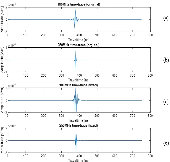
domain. Within this domain the fractures have varying dips, azimuths, radii and aperture-distributions. The borehole consisting of the transmitters and receivers is depicted with the red vertical line. The transmission and detection of the electromagnetic wave then happens according to the effective dipole method depicted in figure 6. ... 16 Figure 9: Time-series representations of both 100MHz and 250MHz of the synthetic GPR responses before

(original) and after (fixed). One can see that the time-windows of the two frequencies are different (see Fig.9a

& 9b) due to the lower-frequency dataset reaching further away from the borehole, resulting in the data not being as comparable as possible for the deep learning algortihm. After increasing the time-window and the sampling-rate both traces are comparable, which results in the deep learning algorithm having more ease in finding the desired transformations between them (see Fig.9c & 9d). ... 18 Figure 10: GPR image representations of both 100MHz and 250MHz of one realization of the synthetic GPR data.

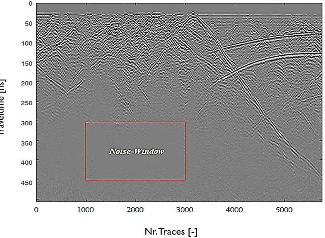
Since GPR images consists of a number of traces stacked together, these images represent a comparable dataset as well, which can be an input for the deep learning algorithm of image-segmentation. ... 20 Figure 11: The noise-window defined in a GPR image obtained from previously obtained data from BULG data in

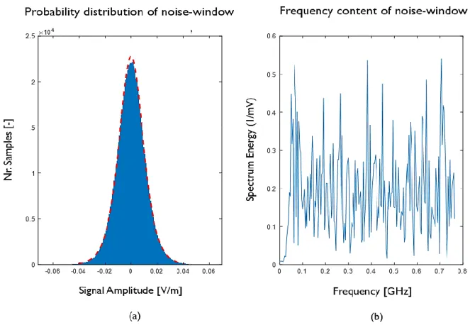
borehole CB1. The larger the travel-time, the further away from the borehole, meaning a lower S/N ratio and more noise. The noise-window then gives information on the noise present in BULG, so that this noise can be replicated and added to the synthetic data. ... 21 Figure 12: The logistic probability distribution (a) and the frequency content (b) of the noise window defined in

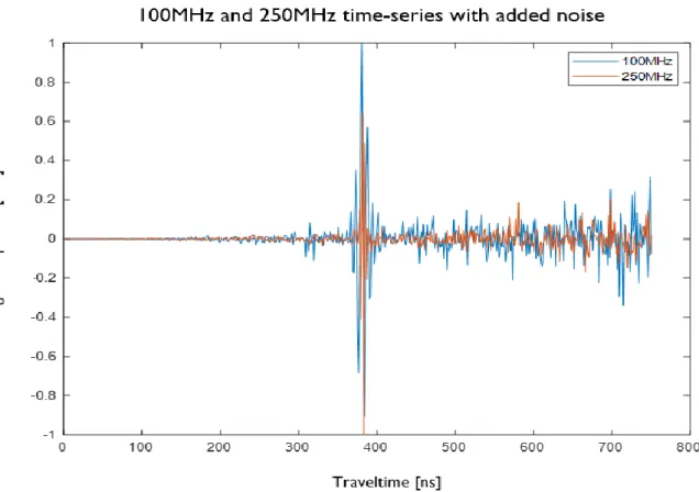
borehole CB1. The random noise in (b) can be re-created with the distribution in (a) and later added to the synthetic data to make it as realistic as possible compared to the field data in BULG. In (a) the blue zones represents the histograms of the values found in the noise window, whereas the red curve is the fitted logistic distribution. The parameters to create this curve are then used for the addition of the noise later on. ... 22 Figure 13: Normalized and comparable time-series representations of the realizations of the 100MHz and

250MHz dataset with the noise added. It is visible that even with the noise added to the synthetic trace, the GPR response of the fracture with heterogeneous aperture distributions is still visible. ... 24 Figure 14: GPR image of one of the realizations of the 100MHz and 250MHz dataset with noise added. These

images are a result of the stacking of the time-series representations such as in Figure 13. ... 24 Figure 15: The super-resolution architecture used during the forward pass. Here every box represents a different

machine learning layer leading to the desired output. ... 25 Figure 16: Reconstruction of the validation loss vs the number of epochs. The loss jumps around over several

orders of magnitude, therefore not gradually decreasing as the number of epochs increases. This means the

(10)

ix model does not learn to make the output closer to the targeted ground-truth; in this case the 250MHz time- series. ... 27 Figure 17: The output of a random time-series representation does not improve during the evaluation of the

obtained model. It can be seen that the energy does not localize, meaning the desired target output is not obtained after the indicated number of epochs. ... 27 Figure 18: The U-Net architecture, where each blue box corresponds to a multi-channel feature mapping. The

number of channels is denoted. on top of the box. The arrows denote the different operations. (Retrieved from Ronneberger et al. 2015) ... 28 Figure 19: GPR responses without added noise of three types of fractures present in the synthetic GPR data. These three types are the basis of the created three categories in order to obtain three image-segmentation models;

one for detecting mainly horizontal structures, one for mainly dipping structures and one for the combination of both. ... 29 Figure 20: Synthetic GPR input image containing a random fracture realization with added noise (a) and its binary

index map which serves as the ground truth that the algorithm needs to learn (b). In the binary index map the yellow zone represents a 100% probability, whereas the purple-blue zone represents a 0% probability. ... 30 Figure 21: Next to having GPR-images containing data as input, Model III also has images containing plain noise

(emulating the noise in BULG) as an input (a). The binary index mapping of this noise can be seen in (b).

When passing the noise through the U-Net, the model then knows how to identify a certain region as noise 31 Figure 22: Validation loss vs epochs. The loss decreases gradually as the number of epochs increases, which means

that the model learns to make the output closer to the targeted ground-truth. The end-loss should therefore be as small as possible. ... 32 Figure 23: The output of a random fracture-realization of Model I improves after each epoch, therefore getting a

smaller loss and a higher Dice-coefficient. The more the model improves, the closer the model-output is to the targeted ground-truth. The different colors in the model output each represent a probability, which can be seen in the color bar; here yellow represents a 100% probability, whereas purple-blue represents a 0%

probability respectively. ... 33 Figure 24: The ground-truths (first tow), noisy inputs (second row) and outputs (third row) of a random fracture-

realization for the thresholding approach and the image-segmentation of Model I using deep neural networks respectively. It is clearly visible that the image-segmentation approach (second column (b)) performs better in terms of visuals and metrics compared to the threshold method (first column (a)), therefore providing a good solution to automatically detect fractures in images of synthetic GPR-datasets. For the final output of Model II and Model III please refer to appendix B. ... 34 Figure 25: Different models of different categories for the input in (a). In (b) one can see the horizontal structures

that get detected by Model I, whereas one can see dipping structures getting detected in (c). In (d) one can see the combination of all structures getting detected as Model III is a combination of all possible structures. In (e) the threshold method is visible, which shows a relatively bigger amount of noise getting displayed. In the models several structures of different intensities are visible according to the color bar, which ranges from a probability of 0% to a probability of 100%. ... 35 Figure 26: Grid of BULG image according to the correct spatial scales. The grid has been numbered with A-F for

the rows and 1-23 for the columns. ... 37 Figure 27: The borehole parallel model (Model I) applied to borehole CB1, resulting in a probability map where

the fractures might be present. Several structures of different intensities are visible according to the color bar, which ranges from a probability of 0% to a probability of 100%. ... 38 Figure 28: The borehole perpendicular model (Model II) applied to borehole CB1, resulting in a probability map

where the fractures might be present. Several structures of different intensities are visible according to the color bar, which ranges from a probability of 0% to a probability of 100%. ... 39 Figure 29: The model that combines all structures (Model III) applied to borehole CB1, resulting in a probability

map where the fractures might be present. Several structures of different intensities are visible according to the color bar, which ranges from a probability of 0% to a probability of 100%. ... 40 Figure 30: Comparison of the models of patches B7-B8-C7-C8 of borehole CB1. ... 41 Figure 31: Comparison of the models of patch E4 of borehole CB1. ... 41 Figure 32: Threshold method applied to borehole CB1. When displaying all the amplitudes above a threshold of

10% of the maximum amplitude one can see several structures get detected, as well as noise. The values depicted are either a value of 0 or 1 as can be seen in the color bar. ... 42

(11)

x Figure 33: Example of a Spectrogram of spoken audio. Frequencies are shown on the vertical axis, whereas time is

shown on the horizontal axis. Certain patterns can be detected by a CNN within such a scalogram, resulting in the network learning the transformation between spectrograms of 100MHz and 250MHz (Retrieved

September 15^th 2020, from Wikipedia.com) ... 46

Figure 34: Borehole CB2 ... 49

Figure 35: Borehole CB3 ... 49

Figure 36: Borehole MB4 ... 50

Figure 37: Final result of Model II applied to a random synthetic fracture realization. As can be seen the output for the threshold method is rather poor in terms in visuals and metrics, therefore confirming the image- segmentation method performs better. ... 51

Figure 38: Final result of Model III applied to a random synthetic fracture realization. Compared to the two previous models, Model III performs better for both the image-segmentation model and the threshold approach. The fact that the threshold approach performs so well in comparison to the two other cases is most likely due to the intensities of the different fractures within the model varying. Since the noise added to all simulations is scaled by 10% of the maximum amplitude present in the data, it is likely to state that this specific fracture realization is one containing one of the highest amplitudes within the entire dataset. Altogether one can still see that the image-segmentation model performs better in terms of visuals and metrics. ... 52

Figure 39: Model I, borehole CB2 ... 53

Figure 40: Model II, borehole CB2 ... 53

Figure 41: Model III, borehole CB2 ... 54

Figure 42: Threshold method, borehole CB2... 54

Figure 43: Model I, borehole CB3 ... 55

Figure 44: Model II, borehole CB3 ... 55

Figure 45: Model III, borehole CB3 ... 56

Figure 46: Threshold method, borehole CB3... 56

Figure 47: Model I, borehole MB4 ... 57

Figure 48: Model II, borehole MB4 ... 57

Figure 49: Model III, borehole MB4 ... 58

Figure 50: Threshold method, borehole MB4 ... 58

(12)

xi

Acronyms and Abbreviations

• ADAM: Adaptive Moment Estimation

• BULG: Bedretto Underground Laboratory for Geo-Energies

• CNN: Convolutional Neural Network

• EGS: Engineered Geothermal System

• FFT: Fast Fourier Transform

• GPR: Ground Penetrating Radar

• MSE: Mean Squared Error

• PDF: Probability Distribution Function

• S/N-ratio: Signal to Noise ratio

• SDL: Soft Dice Loss

• SGD: Stochastic Gradient Descent

(13)

1

1. Introduction

With our climate changing more rapidly than ever and the increased aversion towards nuclear energy, the Swiss government has decided to increase the share of renewable energies for the Swiss Energy Strategy of 2050. This increase in renewable energies has sparked interest in the field of geothermal energy, which can be used for electricity and heat production by utilizing the heat produced and captured deep inside the subsurface. To capture this heat, cold water is injected into the subsurface at high pressure, after which it is pumped back to the surface with higher temperatures. In order to have the most efficient energy transition to properly obtain the goals set for 2050, it is necessary to gain insight on this geothermal approach and its setting.

A part of the currently produced geothermal energy worldwide is acquired in a so-called Engineered Geothermal System (EGS). An EGS is created when the permeability of the rocks in the geothermal environment is low, and by enhancing the permeability of these rocks, more efficient energy extraction can take place. A possible setting for an EGS and the exploitation of geothermal energy is in crystalline rock masses containing fractures and faults. This is mostly due to the fact that they are present in the depths where the EGS is usable. The fractures and faults are the primary conduits for fluid flow and heat transport, making a proper characterization of the fractures and their properties of great importance (e.g. Jefferson et al. 2006).

One way to investigate the fracture network is using Ground Penetrating Radar (GPR) (e.g.

Olsson et al. 1988). GPR offers a non-destructive and cost-effective way of imaging the subsurface using electromagnetic fields, and is able to detect fractures whose apertures are of several orders of magnitude smaller than the dominant wavelength of the GPR antenna (e.g. Shakas and Linde 2017). One has the possibility of recording GPR data in various ways in order to obtain information on the present fracture network, one of them being borehole GPR. The borehole GPR antennae image perpendicular to the borehole in order to map surrounding features in rock-formations and supply information on the desired fracture-properties such as the aperture.

Despite GPR being an excellent way to investigate fractures, one always has to compromise between data resolution and penetration depth of the electromagnetic wave (e.g. Jol 2008). As a rule of thumb one is able to state that the higher the frequency of the antenna, the higher the resolution becomes. From this one can conclude that the higher-frequency GPR acquisitions are able to better detect the fractures close to the borehole wall, but are not able to image as far as the lower-frequency antennae would be able to. This is due to the higher-frequency signals being attenuated.

In order to obtain better knowledge on the fracture network and its properties, one ideally has to be able to detect most of the fractures present in the borehole environment. One can therefore create a way to automatically detect these using the principle of image-segmentation. Additionally one can try to enhance the resolution of the lower-frequency data further away from the borehole to compensate for the shorter penetration depth of the higher-frequency data using the principle of super-resolution. Both these methods enhance the detectability of the fractures. However, GPR data remains difficult to interpret, which is why it is desired to find a way other than using human capabilities to perform these tasks.

(14)

2 Over the past few years deep neural networks have achieved great success in signal- and imaging- processing related fields such as, but not limited to, super-resolution and image enhancement (e.g. Kim et al. 2016). This is why it is of great interest to apply this type of deep neural networks to GPR measurements taken during field-acquisition. One then has the opportunity to enhance the resolution of the lower-frequency data further away from the borehole, as well as trying to detect the fractures in these areas in an automatic fashion.

For the super-resolution task, the deep neural network focuses on creating a mapping between the time-series representations of the lower- and higher- frequency GPR datasets in the areas where the two overlap. Subsequently, one can apply this mapping to regions further away from the borehole where only the lower-frequency data reaches. By applying this mapping the resolution is enhanced. For the image-segmentation task, the deep neural network focuses on creating a pixel-wise probability map of each object within the image of the data. It therefore has the goal of identifying the location and shapes of each object, or in this case fracture reflections, by classifying every pixel of the image within the desired labels. Both the desired mapping and model to automatically detect the fractures within the data can be created by applying several filters and (non-)linear transformations to the time-series representation of lower-frequency data and the image representation of the data respectively (e.g. Sadouk 2018).

In this thesis a detailed look is given at the detection and enhancement of fractures in areas close to and further away from the borehole in GPR data acquired in the Bedretto Underground Laboratory for Geo-Energies (BULG). The deep neural networks are trained with synthetic data that emulates the data from BULG as close as possible, after which the resulting models are applied to the real data from the field. The fact that the deep learning algorithms are trained with synthetic data is due to the neural networks needing a quantity of data for training, which exceeds the achievable quantity of data acquired in BULG. Furthermore, one creates synthetic data in a controlled environment, meaning the parameters to obtain the results are known. This results in one also knowing the location of the fracture reflection, giving one the possibility to later on label the data automatically during the image-segmentation approach. During this thesis all lower- and higher-frequency GPR datasets consist of 100MHz and 250MHz respectively. The image- segmentation approach only makes use of GPR images of 100MHz, whereas the super-resolution approach makes use of both 100MHz and 250MHz datasets.

The final goal of this thesis is to produce two models, one from image-segmentation and one from super-resolution, that enhance the detectability of the fractures in the fracture network of BULG after training them with synthetic data. These models have a better performance compared with human capabilities, therefore providing a better description of the fracture network in the geothermal environment and their changes within.

(15)

3

2. Background theory

This chapter discusses the background theory on GPR, as well as a short recap on electromagnetic theory. Afterwards, the background theory on convolutional neural networks and their training processes will be discussed. With this background knowledge one is able to properly analyze and create the datasets, as will be discussed in chapter 3 and chapter 4.

2.1. Ground Penetrating Radar (GPR)

GPR is a geophysical method which uses electromagnetic fields to probe dielectric materials to detect structures and changes within the material properties of these materials. One application of GPR is to image the subsurface using electromagnetic pulses that are transmitted into the ground and then scattered and/or reflected by changes in the electromagnetic impedance, which gives rise to certain events that appear similar to the emitted signal.

The electromagnetic wave which is transmitted by the transmitter antenna into the subsurface has a certain speed which is influenced by the electric permittivity ε [F/m], relative magnetic permeability μ [H/m], and electrical conductivity σ [S/m] (e.g. Slob et al. 2010).

Once the wave propagates further into the subsurface, the strength of the signal is reduced, mainly due to phenomena such as attenuation, scattering of energy, reflection losses, transmission losses, and geometrical spreading of the energy.

The GPR device which is used during the investigation consists of two antennae; the transmitter antenna that emits the electromagnetic waves and the receiver antenna that then detects the reflected signals from the subsurface structures.

In BULG several boreholes are present in which one can take GPR measurements that are carried out with a transmitter antenna that hangs underneath the receiver antenna with a fixed desired distance. A typical setup for single-borehole GPR acquisition can

be seen in Figure 1. The emitted electromagnetic wave from the transmitter antenna then encounters a fracture and gets reflected back to the receiver antenna, after which the electronics of the system record the data.

Figure 1: Single-borehole GPR measurement set-up.

The transmitter antenna sends out the electromagnetic wave (green), after which the receiver antenna detects the reflected wave (red) from the fracture.

(16)

4 The electromagnetic wave which is emitted from the antenna is composed of oscillating magnetic and electric fields, perpendicular to each other. (e.g. Slob et al. 2010). These oscillations are a result of the electromagnetic wave being a creation of a current flowing into two separate wires that form an electric dipole. (e.g. Bodnar 1993).

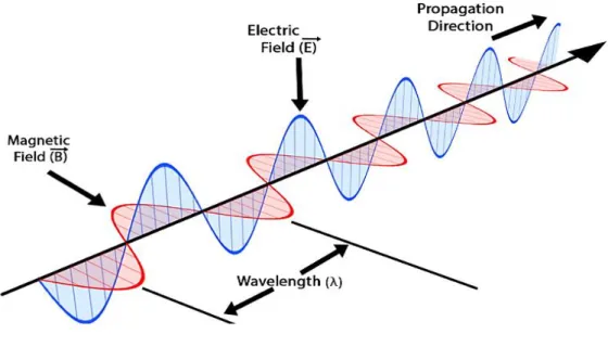
Electromagnetic waves propagate due to the succession of induced field, meaning an electric field generates a magnetic field, whose change then generates an electric field and so on. Since the electric field and the magnetic field are perpendicular with respect to each other, the direction of propagation of the electromagnetic wave can be given by the cross product between the two (see Fig.2)

Fundamental to the description of electromagnetic waves, including waves created from GPR, are the Maxwell Equations and the Material Equations resulting from them (e.g. Slob et al. 2010).

The latter for the magnetic field can be described as the magnetic flux density 𝐵⃗ [𝑇], which is a multiplication between the magnetic permeability 𝜇 and the magnetic field strength 𝐻 ⃗⃗⃗⃗ [A/m] (see Eq. 1). The material equation for the electric field can be represented as the electric flux density 𝐷⃗⃗ [C/m²], which is a multiplication of the (dielectric) permittivity 𝜀 and the electric field strength 𝐸⃗ [V/m] (see Eq. 2). In addition there is Ohm’s law, which describes electric current density 𝐽 [A/m²] as a multiplication between the conductivity 𝜎 and the electric field strength 𝐸⃗ (see Eq. 3).

It is worth noting that when the properties change in space, the multiplications become a convolution.

From these equations one can observe that the propagation of electromagnetic waves is determined by the material properties 𝜇, 𝜀 and 𝜎. The dielectric permittivity 𝜀 and the conductivity 𝜎 mainly determine the refection properties of the subsurface, and thus the contrast between subsurface layers where reflections take place. In the case of BULG the contrast would be between water-filled fractures and homogeneous granite.

Figure 2: Electromagnetic wave propagation (Retrieved August 2nd 2020, from toppr.com )

(17)

5 The permittivity of water-filled fractures is about 10 times higher than the permittivity of the granite, therefore resulting in a high contrast in the data (see Table 2).

𝐵⃗ = 𝜇 ∙ 𝐻⃗⃗ (1)

𝐷⃗⃗ = 𝜀 ∙ 𝐸⃗ (2)

𝐽 = 𝜎 ∙ 𝐸⃗ (3)

From the Maxwell Equations the electromagnetic Wave Equations, which describe the propagation of electromagnetic waves through a medium, are derived (see Eq. 4 and 5).

∇ ²𝐻⃗⃗ = 𝜇𝜎𝜕𝐻⃗⃗

𝜕𝑡 + 𝜇𝜀𝜕²𝐻⃗⃗

𝑑𝑡²

(4)

∇ ²𝐸⃗ = 𝜇𝜎𝜕𝐸⃗

𝜕𝑡 + 𝜇𝜀𝜕²𝐸⃗

𝑑𝑡²

(5)

𝑣 = 1

√𝜇𝜀 = 𝑓𝜆

√𝜀𝑟

(6)

For both the electric and the magnetic field strength 𝐸⃗ and 𝐻⃗⃗ , the Wave Equation applies in a charge-free space. Subsequently, it becomes evident that the propagation velocity v [cm/s] of the electromagnetic waves is equal to 1 divided by the square root of 𝜀 times 𝜇 (see Eq. 6). Together with the amplitudes of the radar waves, they represent the measurement parameters of GPR.

Common velocities for GPR acquisitions range from 6cm/ns to 15cm/ns, with an average value of 12 cm/ns in homogeneous granite such as in BULG.

The introduction discussed that the penetration depth of the electromagnetic wave gets shortened when increasing the frequency of the antenna. This phenomenon is related to the attenuation α [dB/m] of the electromagnetic energy, meaning that the attenuation defines the continuous loss of amplitude an electromagnetic wave experiences as it travels further into the respective medium.

The attenuation therefore dictates how deep one is able to look inside the formation (see Eq. 7).

Here one assumes the wave-regime approximation where the conductivity σ is smaller than the multiplication between the angular frequency ω [rad/s] and the dielectric permittivity ε: (εω≫σ)

𝛼 = 𝜎 2√𝜇

𝜀 (7)

The attenuation can be described in terms of skin depth, or penetration depth, δ [m] (see Eq. 8).

However, when assuming the respective medium is non-magnetic, one obtains a more general expression for the penetration depth (see Eq. 8.) Here 𝜀_𝑟 represents the relative permittivity [-].

𝛿 = 1 𝛼= 2

𝜎√𝜀

𝜇= 0.0053√𝜀𝑟

𝜎 (8)

(18)

6 Now that the background theory on GPR has been discussed, one can look at the background theory of convolutional neural networks in machine learning.

2.2. Convolutional Neural Networks in Machine Learning

Since one desires models that are able to enhance the detectability of the fractures using image- segmentation and super-resolution, one has to make use of deep learning. Deep learning is a specific class of machine learning which makes use of multiple layers within the architecture to extract higher level features from input data (e.g. LeCun et al. 2015). Traditional fully connected networks containing few layers within the architecture of the algorithm can give results which are, in complicated cases, not yet accurate enough (e.g. Yamashita et al. 2018). In order to obtain accurate results and create the mapping between these lower- and higher-frequency datasets as well as the automatic fracture-detector, deep learning needs to be used. Deep learning algorithms which make use of neural networks containing convolutional layers, have achieved extraordinary success for the past few years in the fields of image enhancement, object recognition, signal processing and super-resolution. For this reason it is chosen to utilize these so-called convolutional neural networks (CNN) in order to eventually obtain the desired models.

CNN’s take inputs and assign importance such as weights to certain objects or features within the input data, after which it is able to differentiate one from the other (e.g. Jiuxiang Gu et al. 2017).

These weights are the learnable parameters which function in obtaining the final output. From this it can be seen that CNN’s are designed to automatically and adaptively learn spatial and temporal dependencies, or hierarchies, of certain features from low- to high-level patterns.

Since several features need to be detected in order to obtain a result which captures everything needed for the super-resolution and image-segmentation, one needs to make use of several (convolutional) layers. Another benefit of the CNN is that it uses weight-sharing, meaning that not every node in the network needs to be connected to every single node in the next layer (e.g.

Takahashi et al. 2019). This approach cuts down the number of weight-parameters required to train the model and speeds up the computation time.

In order to create the right CNN-algorithms, optimization techniques and implement the correct methodologies in solving the prediction problems, one needs to have a proper understanding on the type of deep learning problem one is dealing with. The next sub-section discusses two techniques in (supervised) machine learning to achieve this.

2.2.1. Regression and Classification

In supervised machine learning one has a set of labelled data, meaning the values of the input variables and the output variables are known. Since the two desired final models of this thesis make predictions where the fractures are present and how the higher resolution time-series look like, one has to work with supervised machine learning. Here an algorithm is employed to learn a mapping function from the input variable to the output variable. In doing so one can finally obtain a result as accurately as possible, such that when one utilizes a new input the corresponding output can be predicted. Under supervised machine learning one makes a differentiation between two techniques; regression and classification (Bishop et al. 2006).

The main difference between regression and classification problems is that the output variable in regression is continuous, whereas the output for classification is discrete. In other words;

regression algorithms attempt to estimate the desired mapping function to numerical output variables compared to categorial output variables for classification algorithms.

(19)

7 Hence, one can state that the super-resolution problem needs a regression algorithm since it tries to predict how a time-series representation of a corresponding higher frequency GPR dataset looks. The image-segmentation then needs a classification algorithm since it automatically tries to detect the fractures in a given GPR image. A more detailed explanation on the specific type of architecture for each respective method will be given in chapter 4. Once the problem is identified, one is able to construct the right kind of deep learning neural network such as a CNN. The following sub-section focuses on typical operations and characteristics found in a CNN.

2.2.2. General overview of training a CNN

A CNN often consists of an input and an output layer, containing multiple hidden layers in between them. These hidden layers make use of convolutional operations that can be seen as cross-correlations (e.g. Jiuxiang Gu et al. 2017). The output of each of these layers is fed as an input to the next layer, which makes the extracted features able to hierarchically and progressively be turned more complex. In doing so, the algorithm can learn to detect complex patterns which is desired for the image-segmentation and super-resolution approaches.

The common workflow of CNN’s, and deep neural networks in general, starts with a random model initialization.

The reason one performs a random initialization is that one can eventually reach the pseudo-ideal model wherever one starts. Subsequently, one passes the data through the architecture where one checks its performance during a forward pass. Once this has been performed, one is able to check the difference of the output from the forward pass with the targeted output. This performance is evaluated with

a loss-function, which tells how well the network manages to reach a goal as close as possible to the desired value. Since one desires the loss to be as small as possible, optimization is performed by modifying the internal weights by the means of differentiation of the loss function.

When the derivative, which essentially is the rate of which the error changes relative to the weight changes, is decomposable, one is able to perform back-propagation of the errors. This ensures that the next forward pass performs better, resulting in a smaller error. Subsequently the weights of the neural network can then be updated, hence improving the model. For the updating of the weights the delta rule is used (see Eq. 9). This equation shows that the new and updated weight can be obtained by taking the old weight and subtracting the derivative multiplied by the learning rate from it. Here the learning rate is a constant value which forces the weight to get updated smoothly therefore improving the model. Ultimately one has to perform the entire process for several iterations in order to let the model converge. An overview of the forward and backward paths including the weight-updates can be seen in Figure 3.

Figure 3: Schematic overview of forward and backward paths during training of the CNN. The input gets passed through the model architecture, after which the output gets compared with the desired output using the loss function. The derivative of this loss is then used during optimization to update the weights that are used during the next forward pass.

(20)

8 New weight = old weight-(derivative of loss function*learning rate) (9) Figure 3 shows that during the forward pass the input data is put through a certain architecture.

In this architecture several operations and (non)-linear transformations are performed, after which the models gets optimized using the derivative of the loss function. The following subsections discuss the thought behind these typical and common operations performed in working with and creating a CNN applicable for the research in this thesis.

2.2.2.1. Convolutional layers

The main purpose of the convolutional operation is to extract features from the input. The more convolutions one performs, the more features one can extract and the better the network becomes at recognizing patterns such as fractures in a given image. The element of the convolution operation that carries out the convolution itself is called the kernel. This kernel can have a certain size, or dimension, depending on the input and desired output. It performs a matrix multiplication operation between itself and the portion of the input data over which the kernel is hovering (Bishop et al. 2006). This is the reason why a convolutional operation can also be seen as a cross-correlation. Convolutional operations are able to extract different types of features such as edges and curves (Bishop et al. 2006).The more high-level features get extracted, the more the input data gets down-sampled. However, if one desires the output to be of the same size as the input, one also needs to up-sample the data again to ensure a valid comparison in the loss- function. This up-sampling is performed using transposed convolutions. Transposed convolutions are often used in modern image-segmentation and super-resolution problems in machine learning (Ronneberger et al. 2015).

Since the convolution is a linear operation, due it being an element wise matrix multiplication and addition, one also needs to add non-linearity into the model. This is done using an activation layer, as described in the next subsection.

2.2.2.2. (Non-linear) activation layers

The non-linear activation function can be seen as a gateway between the input from the previous layer of the current neuron and the output going into the next layer. The purpose of this activation layer is to introduce non-linearity into the model (Bishop et al. 2006). The non-linear activation function is often represented by a so-called ReLU layer, which stands for a rectified linear unit layer. The ReLU is computationally efficient and has proved to perform well in most deep learning research due to its simplicity (e.g. Takahashi et al. 2019).

Another documented reason the ReLU works well is due to its derivative not suffering from the vanishing gradient problem. The vanishing gradient problem occurs when many derivatives close to zero get multiplied together due to backpropagation. Other activation functions such as Tanh and Sigmoid experience this problem (e.g. Takahashi et al. 2019).

After the convolutional and ReLU operation, one obtains an output that is also known as a rectified feature map. One can apply several more operations on this output, of which the most common ones are briefly mentioned in the following subsections.

(21)

9 2.2.2.3. (Max)-pooling layers

Spatial pooling reduces the dimensionality of the feature map, but is able to retain most of the important information. This results in more ease in training the network. In case of max-pooling operations the dimensionality is reduced by partitioning the feature map into several blocks and picking the maximum value from that block to pass it on. The pooling operation therefore has the goal to make the input smaller and more manageable, reduce the number of parameters to ensure faster computation, avoid overfitting and help to achieve an almost equivariant representation of our data (e.g. Hinton et al. 2012).

After reducing the dimensionality of the feature map one can apply several more operations in speeding up the training of the model. Two of those, which are later used in the architectures of our algorithms, are briefly mentioned in the following two subsections.

2.2.2.4. Batch-normalization layers

When there are several layers stacked on top of each other in the models architecture, each layer’s input is affected by the parameters of all the preceding layers (Ioffe and Szegedy, 2015).

This means that during training each layer has to continuously adapt to the new distribution obtained from the previous layer, which slows down the convergence. Batch-normalization layers overcome this issue by normalizing the layers input in batches and serve in the process of speeding up the performance and regularization. Regularization is used to avoid the overfitting of the data when it is passed through the CNN by reducing and simplifying the model, therefore preventing the model from overworking and capturing data that does not represent the true properties. (Ioffe and Szegedy, 2015). Since normalization is performed in batches, the gradient of the loss is also estimated over batches instead of the entire training set, therefore speeding up the computations.

2.2.2.5. Drop-out layers

Next to batch-normalization, another technique to avoid this overfitting is to randomly drop out nodes during training, therefore simplifying the model and improving training. One often makes use of a combination of drop-out layers with batch-normalization in order to ensure some regularization to fix the overfitting of the model and speed up the convergence. (Chen et al. 2019).

2.2.3. Optimization (back-propagation)

After passing the input data through several layers which detect the features in the datasets, the training of the model has started since it underwent a forward-pass (see Fig. 3). The algorithm learns by utilizing a loss function that evaluates how well the algorithm is in predicting the output.

The goal is to get a number from the loss-function that is as low as possible, meaning the predicted output is similar to the targeted output. The model can then be optimized using the derivative of the loss function during back-propagation. Back-propagation is performed to calculate the gradients of the loss with respect to all the weights in the network and uses gradient descent to update all the weights to minimize the loss in the next forward pass.

A common loss-function used in super-resolution problems is the Mean Square Error (MSE), whereas the image-segmentation problems often make use of the Soft Dice Loss (SDL).

The MSE is measured as the average of the squared differences between the prediction of the algorithm and the targeted output (see Eq. 10). Here n represents the number of data points, 𝑌_𝑖 the observed output from the algorithm, in this case the 100MHz trace transformed into a 250MHz trace, and Ŷ_𝑖 the target output-trace of 250MHz.

(22)

10 𝑀𝑆𝐸 = 1

𝑛∑(𝑌_𝑖− Ŷ_𝑖)²

𝑛

𝑖=1

(10)

𝑆𝐷𝐿 = 1 − 2 ∑ Ŷ_𝑛 _𝑖𝑌_𝑖

∑ Ŷ𝑛 _𝑖+ ∑ 𝑌_𝑛 _𝑖 (11)

Dice Coefficient

=

^{2 ∑ Ŷ}^𝑛 ^𝑖^𝑌^𝑖

∑ Ŷ_𝑛 _𝑖+ ∑ 𝑌_𝑛 _𝑖 (12)

The SDL function can be seen in Equation (11), where n represents the number of pixels, 𝑌_𝑖 the observed output from the algorithm, in this case the image of the GPR data transformed into a probability map, and Ŷ_𝑖 the target output which is the pixel-wise mask. The number which gets subtracted from the number 1 is the Dice-coefficient (see Eq. 12). This coefficient is defined as two times the overlapping area between the predicted model-output and the ground-truth divided by the total area of the predicted output and ground-truth. It can be used as a metric to evaluate the performance of the algorithm and ranges between 0 and 1, where 1 denotes a perfect and complete overlap. (Murguía and Villaseñor 2003). More on this metric is discussed in chapter 4.

In order to get a low number for both loss-functions, one has to optimize the algorithms using an optimizer, such as the Stochastic Gradient Decent (SGD) or Adaptive Moment Estimator (ADAM). They use gradient descent in order to update the weights of the network (see Fig.3).

The SGD makes use of iterations in a stochastic approximation of a gradient descent optimization-problem, rather than using its actual gradient to update the weights (e.g. Ruder, 2016). This is very convenient when one uses large datasets. During SGD the algorithm selects a number of samples in a random fashion, rather than utilizing the entire dataset, therefore speeding up the process as well.

The SGD optimization maintains a single learning rate that determines the step size at each iteration while moving towards the minimum of the loss function for all weighted updates. One can fix this by applying a decay of the learning rate after a number of iterations, but one can also work with ADAM. This is essentially is an adaptive learning rate optimization algorithm that has been designed specifically for training deep neural networks (Kingma and Ba, 2014). ADAM makes use of the squared gradients to scale the learning rate and utilizes the moving average of that gradient instead of the gradient itself. Both SGD and ADAM provide an update of the weights, therefore ensuring a better output in the next forward pass (see Fig.3).

Now that the background theory on CNN’s and their operations have been discussed, one is able to have a look at the datasets used in this thesis. The following chapter discusses the GPR datasets obtained in BULG, after which synthetic data is created to replicate this field data as close as possible with the purpose of serving as input of the CNN for training.

(23)

11

3. Datasets

3.1. Field data

Before one can create synthetic fractures and their GPR responses under a controlled environment, one first has to have a good understanding of what the fractures and their GPR responses would look like in BULG itself. The following sub-sections discuss the geological environment of BULG, as well as the acquisition of GPR data in more detail. Subsequently, one is able to create synthetic data replicating the field data measured in BULG in order to use it as an input for the CNN.

3.1.1. Geological overview

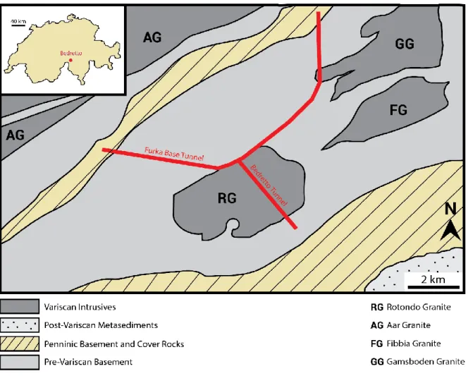
BULG is located in the Bedretto tunnel, which is situated in the Bedretto valley located in the Canton of Ticino in Switzerland. The Bedretto tunnel is located underneath the Pizzo Rotondo mountain in the Lepotine Alps and runs through the Gotthard massif. The Gotthard massif is predominantly comprised of the Pre-Variscan basement consisting of biotite-plagioclase gneisses, schists, amphibolites, serpentinites and eclogites (Lutzenkirchen et al. 2011). This basement was later intruded by several granite bodies after the main stage of the Variscan orogeny (Lutzenkirchen 2002).

Figure 4: Geological mapping of the Bedretto area, highlighting the location of the Bedretto tunnel and the geological formations such as Pre-Variscan gneiss to Variscan granite (Rotondo Granite)

(24)

12 It is known that these homogeneous granite bodies, also known as the Rotondo-Granite, confiscate the largest part of BULG, resulting in the GPR measurements being conducted in homogeneous granite (see Fig.4). Here, faults and fractures act as the primary conduits for heated fluids thus being the primary object of interest for this research.

3.1.2. Data acquisition in BULG

The fractures present in the homogeneous granite formations in BULG are investigated using the previously explained (borehole) GPR measurements. There are several boreholes present in BULG in which measurements have been conducted with 100MHz and 250MHz GPR-antennae (see Table 1).

Figure 5 shows an image of (post-processed) GPR data obtained from borehole CB1 in BULG.

Here one can observe several patterns which might be fractures. The horizontal axis represents the number of traces, whereas the vertical axis represents the travel-time in nanoseconds. One can observe that the bigger the travel-time becomes, the less data is visible and the noisier the data becomes, therefore getting a lower Signal-to-Noise (S/N)-ratio.

Figure 5: A GPR image of 100MHz GPR data from BULG measured in borehole CB1. Some structures and patterns are visible closer to the top of the image (closer to the borehole). However, the further towards the bottom of the image, further away from the borehole, the structures become unclear and covered in noise. For the GPR images of boreholes CB2, CB3 and MB4 please refer to appendix A.

(25)

13 Table 1: Properties of four boreholes present BULG; CB1, CB2, CB3 and MB4.

Borehole Length [m] Diameter [mm] Azimuth [° ] Dip (from horizontal towards dipping) [° ]

CB1 302 98 227.83 45

CB2 222 98 226.81 50

CB3 192 98 225.66 40

MB4 185 175 226.90 49

Section 2.1. discussed that the propagation of electromagnetic waves is determined by the material properties 𝜇, 𝜀 and 𝜎, meaning that the material properties of BULG need to be known in order to create synthetic fractures and their GPR responses as identical as possible. The relevant material properties, obtained from previously executed lab experiments and literature, are stated in Table 2. The following section discusses the creation of the synthetic data in more detail.

Table 2: Relevant material properties found in BULG

Material Properties Value

magnetic permeability 𝜇 12.57×10⁻⁷ [H/m]

relative electric permittivity 𝜀_𝑟 of granite 5.5 [-]

relative electric permittivity 𝜀_𝑟 of water 81 [-]

electric conductivity 𝜎 of granite 0.0001 [S/m]

electric conductivity 𝜎 of water 0.1 [S/m]

3.2. Synthetic data

For the creation of the synthetic data in order to emulate the realistic field data from BULG, the values from Table 2 were used. The following sub-sections address the steps taken in order to obtain synthetic data as accurately as possible.

3.2.1. The GPR responses of synthetic fractures

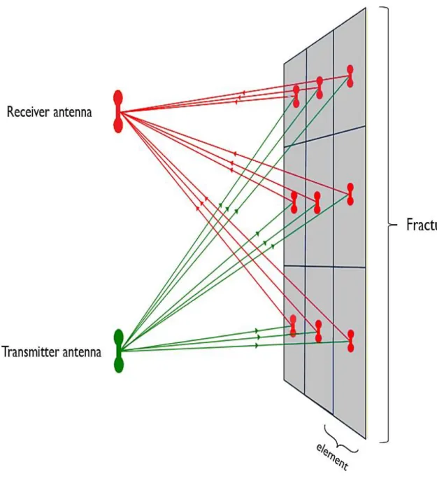
In order to create the synthetic GPR responses of a fracture which is used to feed the algorithm, the effective-dipole method is used. The effective-dipole method is based on an analogy to the microscopic analysis of the Maxwell’s Equations and discretizes a synthetically created fracture into a collection of dipole elements (see Fig.6). This can be done due to the fact that, from a microscopic viewpoint, the electromagnetic waves polarize irregular objects such as fractures filled with fluids (Shakas and Linde, 2015). When discretizing a fracture into elements one has certain advantages such as, but not limited to, taking into account the heterogeneity in fracture fillings and the saving of computation time. The reason one is able to propagate the electromagnetic wave relatively easy using the effective-dipole method lies in the fact that the medium in BULG is comprised of homogeneous granite. This results in it not being necessary to compute every point in space where Maxwell’s Equations need to be determined.

(26)

14 In order to obtain the synthetic source-wavelet which can be used to obtain the GPR responses, one utilizes the borehole wave of previously acquired GPR data from BULG. The borehole wave, or borehole reflection, gives relevant information on the characteristics of the antenna’s source- wavelet. It is, however, not exactly equivalent to the source-wavelet since it is affected by borehole conditions such as presence of water, water-rock interfaces, antenna separation and orientations.

Ergo, one needs to perform normalization with the goal to obtain a good approximation of the source, therefore effectively modeling most of the energy emitted from the source and capturing as much as possible of its frequency content.

Figure 6: Schematic illustration of the effective-dipole forward modeling framework. A fracture is discretized into elements, and each element receives energy (green) directly from the transmitter antenna and radiates (red) back to the receiver antenna (modified after Shakas and Linde, 2017).

(27)

15 It is chosen to perform the normalization using the peak of the energy spectrum of the frequency content in its respective domain for both the 100MHz and 250MHz source-wavelets (see Fig.7).

One then obtains the best-fitting analytical solution which can be used as the source-wavelet.

After obtaining the source wavelet, one is able to then propagate it towards a fracture using the effective dipole method. The obtained source wavelet propagates towards the fracture, after which the facture is polarized and discretized as a collection of dipole elements.

Additionally, one computes the summation of every dipole to each part of the receiver.

The creation of the synthetic fractures is done in an idealized and controlled modeling domain where all the parameters such as the electric properties of the rock matrix and the orientation and position of the fracture itself are known.

The following subsection discusses the creation of the these fractures in more detail.

3.2.2. The creation of the synthetic fractures

In this thesis a modeling domain of 20m x 20m x 10m has been defined, where vertically 20m worth of receiver and transmitter positions were positioned, each having a 10cm spacing (see Fig.8). This results in a total of 201 traces for every GPR response from the synthetic fractures.

The created fractures within the defined domain are created with the properties from Table 2 and have an area of 10m x 10m. Within the defined domain the fracture itself is defined as two rough surfaces with a space-varying separation, also known as the aperture, and with possible contact areas where the aperture is zero.

Certain input parameters have to be defined in order to generate the synthetic fractures which eventually give the GPR responses the algorithm is trained with (see Table 3). The last parameter in the table, namely the aperture, is of great interest since it can define whether a synthetically generated fracture-realization is either homogeneous or heterogeneous in terms of the aperture distribution. More on these two types of fractures and which one of them is more realistic will be briefly discussed in the following sub-sections.

Figure 7: The frequency spectra of the 100MHz and 250MHz borehole data are respectively shown (red). Normalization is performed using the maximum value of the amplitudes, after which one can obtain the best-fitting analytical solution which is used as a source wavelet (blue).This max-energy normalization technique captures the biggest peaks in the frequency content, therefore capturing most information present.

(28)

16 Table 3: Input parameters for the creation of the synthetic fractures

Parameter Value Remarks

Dip 0 - 90 [° ] 0 meaning borehole perpendicular, resulting in horizontal, perpendicular and dipping fractures

Radius 1 – 10 [m] Distance away from the borehole

Azimuth 0 – 25 [° ] Higher azimuths not really detectable Fracture area 10 x 10 [m] Same area for all fractures

Electric conductivity 0.1 [S/m] Electric conductivity of the fracture Relative permittivity 81 [-] Permittivity of the fracture-filling (water) Fracture roughness 0.01 – 0.1 [mm] Only for heterogeneous aperture distributions Mean aperture (1-2.6) × Fracture

roughness [mm]

Only for heterogeneous aperture distributions Correlation length 0.1 – 1 [m] Only for heterogeneous aperture distributions Hurst exponent 0.8 [-] Only for heterogeneous aperture distributions Fracture aperture 0.1 – 10 [mm] Aperture of fracture (either homogeneous or

heterogeneous distribution)

3.2.2.1. Fractures with homogeneous apertures

The first case considered is the case where the synthetic fractures have a homogeneous aperture, meaning the aperture does not vary within the fracture itself. For each synthetically generated fracture, the aperture has a randomly picked constant value in the range between 0.1mm and 10mm (see Table 3).

Nevertheless, apertures of fractures in nature tend to be highly heterogeneous, which leads to one often not using fractures that have apertures with homogeneous values. This is also due to homogeneous fractures with small apertures giving very weak reflections, which are not visible if one later adds noise (e.g. Shakas and Linde 2017).

One ideally wants to simulate fractures that give realistic GPR-reflections similar to the field data in BULG, which is the reason why one also has to create fractures that contain heterogeneous apertures.

Figure 8: A representation of one of the fracture-realizations (depicted in turquoise) within the defined modeling-domain. Within this domain the fractures have varying dips, azimuths, radii and aperture-distributions. The borehole consisting of the transmitters and receivers is depicted with the red vertical line.

The transmission and detection of the electromagnetic wave then happens according to the effective dipole method depicted in figure 6.

(29)

17 3.2.2.2. Fractures with heterogeneous apertures

The second case considered is the case where the synthetic fractures have a heterogeneous aperture distribution, meaning the aperture does vary within the fracture itself. This is the most realistic case since the aperture of fractures in the field is almost never going to be homogeneous.

Before one can create fractures with heterogeneous apertures, one first has to define the heterogeneity. This heterogeneity is characterized by the so-called covariance function that makes use of several extra input-parameters (see Table 3) (Adler & Thovert, 1999). Since the heterogeneous aperture variations exhibit statistically similar patterns over several scales, one can reproduce these fractures mathematically with self-affine functions that create self-affine surfaces.

With these functions one takes the Fast Fourier Transform (FFT) of a 2D Gaussian random field, after which one makes use of an autocorrelation function that has certain input parameters such as the variance, or roughness, σ^h, the cut-off length l^c and the Hurst exponent H (see Eq.

13). The application of the autocorrelation function then makes the respective field correlated.

𝐶_ℎ(𝑢) = 𝜎_ℎ²exp [− (𝑢 𝑙_𝑐)

2𝐻

] (13)

In order to create a fracture with a heterogeneous aperture-distribution, one has to look at the roughness of a fracture surface, which is spatially grouped together over the cut-off length.

Afterwards one can create a top and a bottom surface-area of the fracture using the covariance function with a Hurst exponent of between 0 and 1. Previously obtained experimental evidence suggests that the ratio between the roughness and the mean aperture lies in the region between 0 and 2.6, as well as the ratio between the mean aperture and the correlation length being between 0 and 7 (Adler and Thovert, 1999). From field- and lab-data it can be stated that a Hurst exponent of 0.8 can be used. Using the previously discussed method and parameters, one can create a heterogeneous model describing the local aperture, considering a Hurst exponent of 0.8 and a randomly generated correlation length and roughness (see Table 3).

Performing this results in a fracture with a heterogeneous aperture distribution, therefore emulating the real fractures in BULG. These fractures, as well as the homogeneous case, are then used in the previously discussed effective dipole method, which discretizes the created fractures into elements to compute their GPR response.

The responses of the GPR’s source-wavelet of the fractures are then a result one could feed a deep learning algorithm in the form of either time-series representations or GPR images.

However, before one can do this properly one first has the possibility to adjust the data, making it easier for the deep learning algorithm to perform its task by making the data of both frequencies as comparable as possible. The next section focuses on this in more detail.