Integrating Planning and Learning: The PRODIGY Architecture

Integrating Planning and Learning: The PRODIGY Architecture ¹

Manuela Veloso

Jaime Carbonell

Alicia P´erez

Daniel Borrajo

Eugene Fink

Jim Blythe

School of Computer Science Carnegie Mellon University

5000 Forbes Ave Pittsburgh PA 15213-3891 Phone number: (412) 268 2565

Running head: Planning and Learning: The PRODIGY Architecture.

In Journal of Experimental and Theoretical Artificial Intelligence, 7(1), 1995

1This research is sponsoredby the Wright Laboratory, Aeronautical Systems Center, Air Force Materiel Command, USAF, and the Advanced Research Projects Agency (ARPA) under grant number F33615-93-1-1330. The views and conclusions contained in this document are those of the authors and should not be interpreted as necessarily representing the official policies or endorsements, either expressed or implied, of Wright Laboratory or the U. S. Government. The third and fourth authors were supported by fellowships from the Ministerio de Educaci´on y Ciencia of Spain.

2Current address: Facultad de Inform´atica, Universidad Polit´ecnica de Madrid, Campus de Montegancedo s/n, Boadilla del Monte, 28660 Madrid (Spain).

Abstract

Planning is a complex reasoning task that is well suited for the study of improving performance and knowledge by learning, i.e. by accumulation and interpretation of planning experience.

is an architecture that integrates planning with multiple learning mechanisms. Learning occurs at the planner’s decision points and integration in

is achieved via mutually interpretable knowledge structures.

This article describes the

planner, briefly reports on several learning modules developed earlier

along the project, and presents in more detail two recently explored methods to learn to generate plans

of better quality. We introduce the techniques, illustrate them with comprehensive examples, and show

prelimary empirical results. The article also includes a retrospective discussion of the characteristics of the

overall

architecture and discusses their evolution within the goal of the project of building a large

and robust integrated planning and learning system.

1 Introduction

The

architecture was initially conceived by Jaime Carbonell and Steven Minton, as an Artificial Intelligence (AI) system to test and develop ideas on the role of machine learning in planning and problem solving. In general, learning in problem solving seemed meaningless without measurable performance improvements. Thus,

was created to be a testbed for the systematic investigation of the loop between learning and performance in planning systems. As a result,

consists of a core general- purpose planner and several learning modules that refine both the planning domain knowledge and the control knowledge to guide the search process effectively.

In the first design of

, several simplifying assumptions were made in the planning algorithm, as the focus was to study how to integrate learning and planning. Thus, the first planner in

,

PRODIGY

2.0, assumed linear subgoaling decomposition, i.e., no interleaving of subplans (Minton et al., 1989). The first learning technique developed was explanation-based learning of control knowledge to guide the search process. This first version of the architecture led Minton to complete an impressive thesis with an extensive empirical analysis of the effect of learning control knowledge in the planner’s performance (Minton, 1988a).

After Minton’s successful and pioneering results on incorporating learning into the planning framework, we pursued the investigation of alternative learning techniques in

to address domains and problems of increasing complexity. This led to the need to evolve the

’s planning algorithm from the simple linear and incomplete

2.0 to the current nonlinear and complete

4.0.

The current

architecture encompasses several learning methods that improve the performance of the core planner along several different dimensions.

The article is organized in six sections. Section 2 presents the planner,

4.0. Section 3 describes the learning opportunities that we have addressed in

and briefly reviews all of the learning methods of

. To illustrate concretely how learning is integrated with planning in

, Section 4 presents the techniques to learn to improve the quality of the plans produced by the planner. Section 5 discusses some of the characteristics of the

architecture, shows the evolution of the system in the pursuit of our goal of building a large and robust planning and learning system, and takes a retrospective look at the project. Finally Section 6 draws conclusions on the article.

2 The PRODIGY Planning Algorithm

A planning domain is specified to the

’s planner mainly as a set of operators. Each operator corresponds to a generalized atomic planning action, described in terms of its effects and the necessary conditions which enable the application of the operator. A planning problem in a domain is presented to

PRODIGY

as an initial configuration of the world and a goal statement to be achieved.

The current

4.0 system uses a complete nonlinear planner. It follows a means-ends analysis backward chaining search procedure reasoning about multiple goals and multiple alternative operators relevant to achieving the goals.

4.0’s nonlinear character stems from its dynamic goal selection which enables the planner to fully interleave plans, exploiting common subgoals and addressing issues of resource contention. Operators can be organized in different levels of abstractions that are used by

PRODIGY

4.0 to plan hierarchically.

In this section, we describe how

4.0 combines state-space search corresponding to a simulation

of plan execution of the plan and backward-chaining responsible for goal-directed reasoning. We present a

formal description of

4.0 planning algorithm. We describe and illustrate through a simple example,

the planning domain language used in

. We show how the planner represents incomplete plans

considered during the search for a solution. We presents the technique to change the internal planning

state to simulate the effects of plan execution, and introduce the backward-chaining algorithm. Finally, we discuss the use of control rules in

to guide the search for a solution.

2.1 Domain and Problem Definition

A planning domain is defined by a set of types of objects, i.e., classes, used in the domain, a library of operators and inference rules that act on these objects. Inference rules have the same syntax as operators, hence we do not distinguish them in this section.

’s language for describing operators is based on the

domain language (Fikes and Nilsson, 1971), extended to express disjunctive and negated preconditions, universal and existential quantification, and conditional effects (Carbonell et al., 1992).

Each operator is defined by its preconditions and effects. The description of preconditions and effects of an operator can contain typed variables. Variables can be constrained by functions. The preconditions of an operator are represented as a logical expression containing conjunctions, disjunctions, negations, universal and existential quantifiers. The effects of an operator consist of a set of regular effects, i.e., a list of predicates to be added or deleted from the state when the operator applies, and a set of conditional effects that are to be performed depending on particular state conditions.

When an operator is used in planning, its variables are replaced with specific objects of corresponding types. We say that the operator is instantiated. The precondition expression and the effects of an instantiated operator are then described in terms of literals, where the term literal refers to a predicate whose variables are instantiated with specific objects. In order to apply an instantiated operator, i.e., to execute it in the internal state of the planner, its preconditions must be satisfied in the state. Its effects specify the set of literals that must be added and deleted to the state.

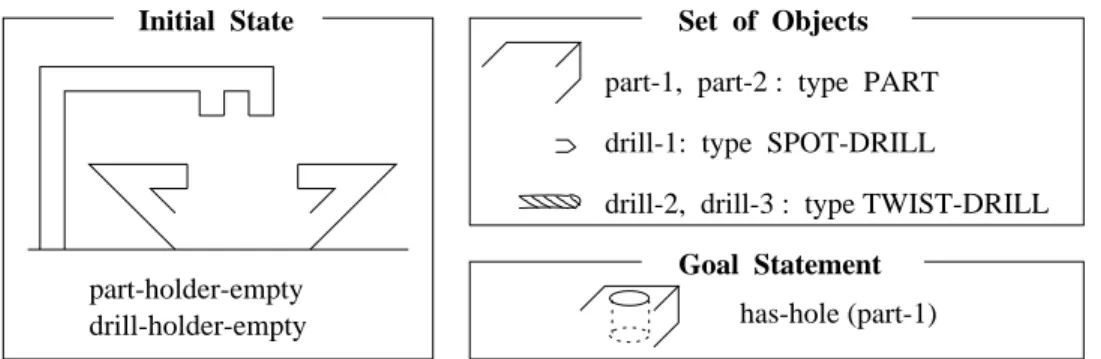
Figure 1 shows an example of a planning domain, a simplified version of a compex Process Planning domain introduced in (Gil, 1991). (In Section 4, we use examples from the complete version of this domain to describe techniques for learning control rules.) This simplified domain represents operations of a drill press. The drill press uses two types of drill bits: a spot drill and a twist drill. A spot drill is used to make a small spot on the surface of a part. This spot is needed to guide the movement of a twist drill, which is used for drilling a deeper hole.

There are two types of objects in this domain:

and

. The latter type is subdivided into two subtypes,

and

. The use of types combined with functions limits the scopes of possible values of variables in the description of operators.

A planning problem is defined by (1) a set of available objects of each type, (2) an initial state

, and (3) a goal statement

. The initial state is represented as a set of literals. The goal statement is a logical formula equivalent to a preconditions expression, i.e. it can contain typed variables, conjunctions, negations, disjunctions, and universal and existential quantifications. An example of a planning problem is shown in Figure 2. In this example, we have five objects: two metal parts, called

and

, the spot drill

, and two twist drills,

and

.

A solution to a planning problem is a sequence of operators that can be applied to the initial state, transforming it into a state that satisfies the goal. A sequence of operators is called a total-order plan. A plan is valid if the preconditions of every operator are satisfied before the execution of the operator. A valid plan that achieves the goal statement

is called correct.

For example, for the problem in Figure 2, the plan “

,

” is valid, since it can be executed from the initial state. However, this plan does not achieve the goal, and hence it is not correct. The problem may be solved by the following correct plan:

.0/*1*23.405,1#67.*40581*29,:;<.0/*1*2,=*5?>A@0@02&B>C1#6D=05?>8@0@02*90:;E=*5?>A@0@020F3.G81#67.*40581*29;+=*5?>A@0@0290:;

50H3IG,J*H02,=*5?>8@0@A23B>K1#6L=*5?>8@0@02?90:;E.0/*1*2,=*5?>A@,@023B>81#67=*50>A@0@,20M?:;+=*5?>A@0@023NG0@0H67.4A5,1*2?9;+=*5?>A@0@020M:

SPOT-DRILL TWIST-DRILL

<drill-bit>

<part>

DRILL PRESS

PART DRILL-BIT

TYPE HIERARCHY

Pre:

Add:

<part>: type PART

drill-spot (<part>, <drill-bit>)

<drill-bit>: type SPOT-DRILL

Del:

Pre:

Add:

tool-holder-empty tool-holder-empty

<drill-bit>: type DRILL-BIT

Pre:

Add:

part-holder-empty

Del: part-holder-empty

<part>: type PART

Pre:

Add:

Del:

part-holder-empty

<part>: type PART

Del:

Pre:

Add: tool-holder-empty

<drill-bit>: type DRILL-BIT

Pre:

Add:

<drill-bit>: type TWIST-DRILL

<part>: type PART

drill-hole(<part>, <drill-bit>)

(holding-tool <drill-bit>) (holding-part <part>) (has-spot <part>)

(has-spot <part>) (holding-tool <drill-bit>) (holding-part <part>) (has-hole <part>)

(holding-tool <drill-bit>)

(holding-tool <drill-bit>)

(holding-tool <drill-bit>)

(holding-part <drill-bit>)

(holding-part <drill-bit>)

(holding-part <drill-bit>) Figure 1: A simplified version of the Process Planning domain.

part-holder-empty drill-holder-empty

drill-1: type SPOT-DRILL part-1, part-2 : type PART

drill-2, drill-3 : type TWIST-DRILL

Goal Statement

has-hole (part-1)

Figure 2: A problem in the simplified Process Planning domain.

A partial-order plan is a partially ordered set of operators. A linearization of a partial-order plan is a total order of the operators consistent with the plan’s partial order. A partial-order plan is correct if all its linearizations are correct. For example, the first two operators in our solution sequence need not be ordered with respect to each other, thus giving rise to the partial-order plan in Figure 3.

put-part (part-1)

put-drill (drill-1) drill-spot (part-1, drill-1)

Figure 3: First operators in the example partial orden plan.

2.2 Representation of Plans

Given a problem, most planning algorithms start with the empty plan and modify it until a solution plan is

found. A plan may be modified by inserting a new operator, imposing a constraint on the order of operators

in the plan, or instantiating a variable in the description of an operator. The plans considered during the search for a solution are called incomplete plans. Each incomplete plan may be viewed as a node in the search space of the planning algorithm. Modifying a current incomplete plan corresponds to expanding a node. The branching factor of search is determined by the number of possible modifications of the current plan.

Different planning systems use different ways of representing incomplete plans. A plan may be presented as a totally ordered sequence of operators (as in Strips (Fikes and Nilsson, 1971)) or as a partially ordered set of operators (as in Tweak (Chapman, 1987),

(Tate, 1977), and

(McAllester and Rosenblitt, 1991)); the operators of the plan may be instantiated (e.g. in

(Veloso, 1989)) or contain variables with codesignations (e.g. in Tweak); the relations between operators and the goals they establish may be marked by causal links (e.g. in

and

).

In

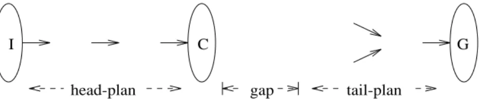
, an incomplete plan consists of two parts, the head-plan and the tail-plan (see Figure 4).

The tail-plan is built by a partial-order backward-chaining algorithm, which starts from the goal statement

and adds operators, one by one, to achieve preconditions of other operators that are untrue in the current state, i.e. pending goals.

I C G

head-plan gap tail-plan

Figure 4: Representation of an incomplete plan.

The head-plan is a valid total-order plan, that is, a sequence of operators that can be applied to the initial state

. All variables in the operators of the head-plan are instantiated, that is, replaced with specific constants. The head-plan is generated by the execution-simulating algorithm described in the next subsection. If the current incomplete plan is successfully modified to a correct solution of the problem, the current head-plan will become the beginning of this solution.

The state achieved by applying the head-plan to the initial state is called the current state. Notice that since the head-plan is a total-order plan that does not contain variables, the current state is uniquely defined.

The back-chaining algorithm responsible for the tail-plan views as its initial state. If the tail-plan cannot be validly executed from the current state ,then there is a “gap” between the head and tail. The purpose of planning is to bridge this gap.

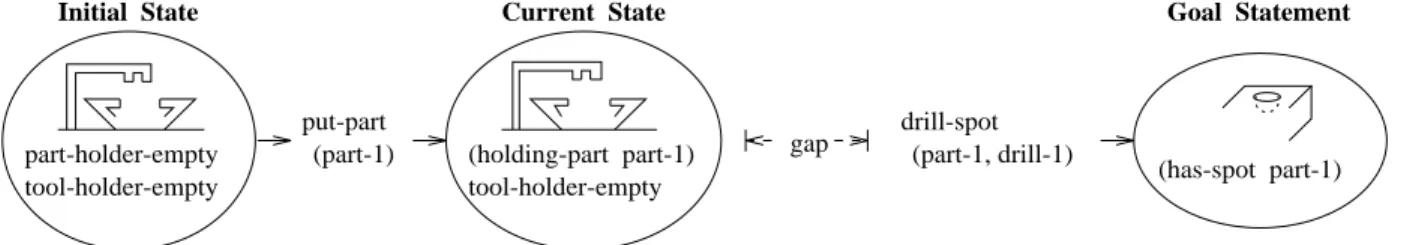
Figure 5 shows an example of an incomplete plan. This plan can be constructed by

while solving the problem of making a spot in

. The gap in this plan can be bridged by a single operator,

"(

?)

*+$A '

.

2.3 Simulating Plan Execution - State Space Search

Given an initial state

and a goal statement

,

starts with the empty plan and modifies it, step by step, until a correct solution plan is found. The empty plan is the root node in

’s search space. The head and tail of this plan are, naturally, empty, and the current state is the same as the initial state,

.

At each step,

can modify a current incomplete plan in one of two ways (see Figure 6). It can

add an operator to the tail-plan (operator t in Figure 6). Modifications of the tail are handled by a backward-

chaining planning algorithm, called Back-Chainer, which is presented in the next subsection.

can

also move some operator op from the tail to the head (operator x in Figure 6). The preconditions of op must

tool-holder-empty part-holder-empty

put-part (part-1)

tool-holder-empty

gap drill-spot (part-1, drill-1)

Initial State Current State Goal Statement

(holding-part part-1)

(has-spot part-1)

Figure 5: Example of an incomplete plan.

be satisfied in the current state . op becomes the last operator of the head, and the current state is updated to account for the effects of op. There may be several operators that can be applied to the state. There are usually also many possible goals to plan for, and operators and instantiations of operators that can achieve each particular goal. These choices are made while expanding the tail-plan.

I s C G

x

y z

t

Adding an operator to the tail-plan

I C G

x

y z

s

I s x C’ y z G

Applying an operator (moving it to the head)

Figure 6: Modifying the current plan.

Intuitively, one may imagine that the head-plan is being carried out in the real world, and

has already changed the world from its initial state

to the current state . If the tail-plan contains an operator whose preconditions are satisfied in ,

can apply it, thus changing the world to a new state, say

. Because of this analogy with the real-world changes, the operation of moving an operator from the tail to the end of the head is called the application of an operator. Notice that the term “application” refers to simulating an operator application. Even if the application of the current head-plan is disastrous, the world does not suffer:

simply backtracks and considers an alternative execution sequence.

Moving an operator from the tail to the head is one way of updating the head-plan.

can perform additional changes to the state adding redundant explicit information by inference rules.

PRODIGY

recognizes a plan as a solution of the problem if the head-plan achieves the goal statement

, i.e. the goal statement is satisfied in .

may terminate after finding a solution, or it may search for another plan.

Table 1 summarizes the execution-simulating algorithm. The places where

chooses among sev- eral alternative modifications of the current plan are marked as decision points. To guarantee completeness,

PRODIGY

must consider all alternatives at every decision point.

Notice that, by construction, the head-plan is always valid.

terminates when the goal statement

is satisfied in the current state , achieved by applying the head-plan. Therefore, upon termination, the

head-plan is always valid and achieves

, that is, it is a correct solution of the planning problem. We

conclude that

is a sound planner, and its soundness does not depend on Back-Chainer.

Prodigy

1. If the goal statement

is satisfied in the current state , then return Head-Plan.

2. Either

(A) Back-Chainer adds an operator to the Tail-Plan, or

(B) Operator-Application moves an operator from Tail-Plan to Head-Plan.

Decision point: Decide whether to apply an operator or to add an operator to the tail.

3. Recursively call Prodigy on the resulting plan.

Operator-Application

1. Pick an operator op in Tail-Plan which is an applicable operator, that is (A) there is no operator in Tail-Plan ordered before op, and

(B) the preconditions of op are satisfied in the current state . Decision point: Choose an applicable operator to apply.

2. Move op to the end of Head-Plan and update the current state . Table 1: Execution-simulating algorithm.

2.4 Backward-Chaining Algorithm

We now turn our attention to the backward-chaining technique used to construct

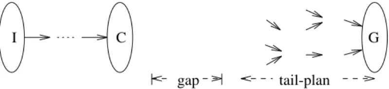
’s tail-plan. The tail-plan is organized as a tree (see Figure 7). The root of the tree is a ficticious operator, *finish*, that adds the goal statement

, the other nodes are operators, and the edges are ordering constraints. Each operator of the tail-plan is added to the tail-plan to achieve a pending goal. Every operator gets instantiated immediately after it is inserted into the tail

.

G

I C

gap tail-plan

Figure 7: Tree-structured tail-plan.

A precondition literal in a tree-like tail-plan is considered unachieved if (1) does not hold in the current state , and

(2) is not linked with any operator of the tail-plan.

When the backward-chaining algorithm is called to modify the tail, it chooses some unachieved literal , adds a new operator op that achieves , and establishes an ordering constraint between op1 and op2. op2 is also marked as the “relevant operator” to achieve l.

Before inserting the operator op into the tail-plan, Back-Chainer substitutes all free variables of op.

Since

’s domain language allows complex constraints on the preconditions of operators, finding the set of possible substitutions may be a difficult problem. This problem is handled by a constraint-based matching algorithm, described in (Wang, 1992).

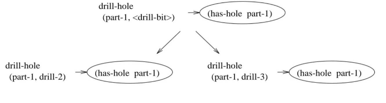
For example, suppose the planner adds the operator

to the tail-

plan in order to achieve the goal literal

, as the effects of the operator unify with the

goal (see Figure 8). First,

instantiates the variable

in the description of the operator with

the constant

from the goal literal. Then the system has to instantiate the remaining free variable,

( !*

. Since our problem contains two twist drills, and

, this variable has two possible instantiations. Different instantiations give rise to different branches of the search space.

drill-hole (part-1, drill-2)

(part-1, <drill-bit>) drill-hole

(part-1, drill-3) drill-hole

(has-hole part-1)

(has-hole part-1) (has-hole part-1)

Figure 8: Instantiating a newly added operator.

A summary of the backward-chaining algorithm is presented in Table 2. It may be shown that the use of this back-chaining algorithm with the execution-simulator described in the previous subsection guarantees the completeness of planning (Fink and Veloso, 1994). Notice that the decision point in Step 1 of the algorithm may be required for the efficiency of the depth-first planning, but not for completeness. If

PRODIGY

generates the entire tail before applying it, we do not need branching on Step 1. We may pick preconditions in any order, since it does not matter in which order we add nodes to our tail-plan.

Back-Chainer

1. Pick an unachieved goal or precondition literal . Decision point: Choose an unachieved literal.

2. Pick an operator op that achieves .

Decision point: Choose an operator that achieves this literal.

3. Add op to the plan and establish a link from op to . 4. Instantiate the free variables of op.

Decision point: Choose an instantiation for the variables of the operator.

Table 2: Backward-chaining algorithm.

2.5 Control Rules

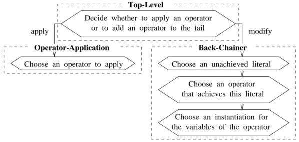
The algorithms presented in the previous section (Tables 1 and 2) determine the search space of the

planner. Different choices in decision points of the algorithms give rise to different ways of exploring the search space. Usually

uses depth-first search to explore its search space. The efficiency of the depth-first search crucially depends on the choices made at decision points. Figure 9 summarizes the decisions made by the system at every step of planning which are directly related to the choice points in Tables 1 and 2.

Strategies used in

for directing its choices in decision points are called control knowledge.

These strategies include the use of control rules (usually domain-dependent) (Minton, 1988a), complete

problem solving episodes to be used by analogy (Veloso and Carbonell, 1993), and domain-independent

heuristics (Blythe and Veloso, 1992; Stone et al., 1994). We focus on explaining control rules.

A control rule is a production (if-then rule) that tells the system which choices should be made (or avoided) depending on the current state , unachieved preconditions of the tail-plan operators, and other meta-level information based on previous choices or subgoaling links. Control rules can be hand-coded by the user or automatically learned by the system. Some techniques for learning control rules are presented in (Minton, 1988a), (Etzioni, 1990) and (P´erez and Etzioni, 1992). In this paper we will present two more rule-learning techniques (see Section 4. Figure 9 shows the decisions made by

, that are also the decisions that can be controlled by control rules. This figure can be very directly compared with Figure 6.

We see that a search node corresponds to a sequence of decisions which will be the learning opportunities.

Choose an operator to apply

Back-Chainer Operator-Application

Choose an operator that achieves this literal Decide whether to apply an operator

or to add an operator to the tail Top-Level

apply modify

Choose an instantiation for the variables of the operator Choose an unachieved literal

Figure 9: Branching decisions.

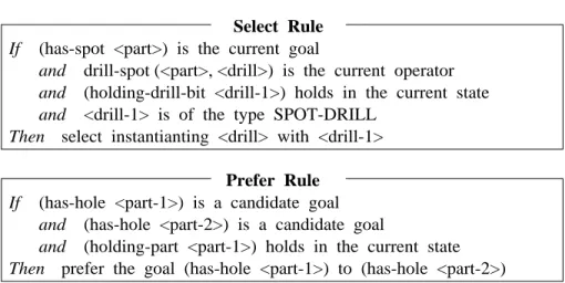
Two examples of control rules are shown in Table 3. The first rule says that if we have just inserted an op- erator

to achieve an unsatisfied goal literal

, and if the literal

is satisfied in the current state for some specific drill

, then we should instantiate the variable

with

, and we should not consider any other instantiations of this variable. This is equivalent to saying that all the drills are identical from this perspective. Thus, this rule selects one of the alternatives and prunes all other branches from the search space. Such a rule is called a select rule. Similarly, we may define a control rule that points out an alternative that should not be considered, thus pruning some specific branch of the search space. The rules of this type are called reject rules.

The second rule in Table 3 says that if we have two unsatisfied goal literals,

and

, and if

is already in the drill press, then the first goal must be considered before the second one. Thus, this rule suggests that some branch of the search space must be explored before some other branch. The rules that provide knowledge on the preferred order of considering different alternatives are called prefer rules.

All control rules used by

are divided into these three groups: select, reject, and prefer rules.

If there are several control rules applicable in the current decision point,

will use all of them.

Select and reject rules are used to prune parts of the search space, while prefer rules determine the order of exploring the remaining parts.

First,

applies all select rules whose if-part matches the current situation, and creates a set of

candidate branches of the search space that must be considered. A branch becomes a candidate if at least one

If and and and

(holding-drill-bit <drill-1>) holds in the current state Then select instantianting <drill> with <drill-1>

Select Rule

If and and Then

(has-hole <part-1>) is a candidate goal (has-hole <part-2>) is a candidate goal

(holding-part <part-1>) holds in the current state prefer the goal (has-hole <part-1>) to (has-hole <part-2>)

Prefer Rule (has-spot <part>) is the current goal

drill-spot (<part>, <drill>) is the current operator

<drill-1> is of the type SPOT-DRILL

Table 3: Examples of control rules.

select rule points to this branch. If there are no select rules applicable in the current decision point, then by default all branches are considered candidates. Next,

applies all reject rules that match the current situation and prunes every candidate pointed to by at least one reject rule. Notice that an improper use of select and reject rules may violate the completeness of planning, since these rules can prune a solution from the search space. They should therefore be used carefully.

After using select and reject rules to prune branches of the search space,

applies prefer control rules to determine the order of exploring the remaining candidate branches. When the system does not have applicable prefer rules, it may use general domain-independent heuristics for deciding on the order of exploring the candidate branches. These heuristics are also used if the applicable prefer rules contradict each other in ordering the candidate branches.

When

encounters a new planning domain, it initially relies on the control rules specified by the user (if any) and domain-independent heuristics to make branching decisions. Then, as

learns control rules and stores problem-solving episodes for analogical case-based reasoning, the domain- independent heuristics are gradually overriden by the learned control knowledge.

3 Learning in PRODIGY

The

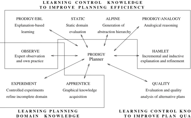
planning algorithm is combined with several learning modules, designed for reducing the planning time, improving the quality of the solution plans, and refining the domain knowledge. Figure 10 shows the learning modules developed in

, according to their learning goal.

We describe briefly some of these algorithms. In the following section, we present in more detail two of

’s learning modules to improve the quality of the plans produced by the planner.

3.1 Learning Control Knowledge to Improve Planning Efficiency

The following are

’s learning modules to acquire control knowledge to improve planning efficiency:

EBL: An explanation-based learning facility (Minton, 1988a) for acquiring control rules from a problem-

solving trace.

analyzes the search space of the planning algorithm and explains the reasons for

branching decisions made during the search for a solution. The resulting explanations are expressed

in the form of control rules.

Graphical knowledge APPRENTICE

acquisition EXPERIMENT

Controlled experiments refine incomplete domain

QUALITY Evaluation and quality analysis of alternative plans OBSERVE

Expert observation and own practice

Static domain evaluation

STATIC PRODIGY/ANALOGY

Analogical reasoning

Planner

D O M A I N K N O W L E D G E

L E A R N I N G P L A N N I N G L E A R N I N G C O N T R O L K N O W L E D G E T O I M P R O V E P L A N Q U A L I T Y Explanation-based

PRODIGY/EBL

learning

PRODIGY ALPINE Generation of abstraction hierarchy

Incremental and inductive HAMLET

explanation and refinement T O I M P R O V E P L A N N I N G E F F I C I E N C Y

L E A R N I N G C O N T R O L K N O W L E D G E

Figure 10: The learning modules in the

architecture. We identify three classes of learning goals:

learn control knowledge to improve the planner’s efficiency in reaching a solution to a problem; learn control knowledge to improve the quality of the solutions produced by the planner; and learn domain knowledge, i.e., learn or refine the set of operators specifying the domain.

STATIC: A method for learning control rules by analyzing

’s domain description prior to plan- ning. The

program produces control rules without analizing examples of planning problems.

Experiments show that

runs considerably faster than

, and the control rules found by

are usually superior to those generated by

. However, some rules cannot be found by

and require

’s dynamic capabilities to learn them.

’s design is based on a detailed predictive theory of

, described in (Etzioni, 1993).

DYNAMIC: A technique that combines

and

. Training problems pinpoint learning opportunities but do not determine

’s explanations.

uses the analysis algorithms introduced by

but relies on training problems to achieve the distribution-sensitivity of

(P´erez and Etzioni, 1992).

ALPINE: An abstraction learning and planning module (Knoblock, 1994).

divides the description of a planning domain into multiple levels of abstraction. The planning algorithm uses the abstract description of the domain to find an “outline” of a solution plan and then refines this outline by adding necessary details.

ANALOGY: A derivational analogy engine that solves a problem using knowledge about similar problems

solved before (Veloso and Carbonell, 1990; Veloso, 1992). The planner records the justification for

each branching decision during its search for a solution. Later, these justifications are used to guide

the search for solutions of other similar problems.

3.2 Learning Domain Knowledge

Acquiring planning knowledge from experts is a rather difficult knowledge engineering task. The following learning modules support the user with the specification of domain knowledge, both at acquisition and refinement times.

EXPERIMENT: A learning-by-experimentation module for refining the domain description if the proper- ties of the planning domain are not completely specified (Carbonell and Gil, 1990; Gil, 1992). This module is used when

notices the difference between the domain description and the behavior of the real domain. The experiment module is aimed at refining the knowledge about the properties of the real world rather than learning control knowledge.

OBSERVE: This work provides a novel method for accumulating domain planning knowledge by learning from the observation of expert planning agents and from one’s own practice. The observations of an agent consist of: 1) the sequence of actions being executed, 2) the state in which each action is executed, and 3) the state resulting from the execution of each action. Planning operators are learned from these observation sequences in an incremental fashion utilizing a conservative specific-to-general inductive generalization process. Operators are refined and new ones are created extending the work done in EXPERIMENT. In order to refine the new operators to make them correct and complete, the system uses the new operators to solve practice problems, analyzing and learning from the execution traces of the resulting solutions or execution failures (Wang, 1994).

APPRENTICE: A user interface that can participate in an apprentice-like dialogue, enabling the user to evaluate and guide the system’s planning and learning. The interface is graphic-based and tied directly to the planning process, so that the system not only acquires domain knowledge from the user, but also uses the user’s advices for guiding the search for a solution of the current problem (Joseph, 1989; Joseph, 1992).

All of the learning modules are loosely integrated: they all are used with the same planning algorithm on the same domains. The learned control knowledge is used by the planner.

We are investigating ways to integrate the learning modules understanding the tradeoffs of the conditions for which each individual technique is more appropriate. Learning modules will then share the generated knowledge with each other and a tighter integration will be achieved. As an initial effort in this direction,

was used in combination with the abstraction generator to learn control rules for each level of abstraction.

The integration of these two modules in

2.0 simplifies the learning process and results in generating more general control rules, since the proofs in an abstract space contain fewer details (Knoblock et al., 1991).

4 Learning to Improve Plan Quality

Most of the research on planning so far has concentrated on methods for constructing sound and complete planners that find a satisficing solution, and on how to find such a solution efficiently (Chapman, 1987;

McAllester and Rosenblitt, 1991; Peot and Smith, 1993). Accordingly most of our work on integrating

machine learning and planning, as described above, has focused on learning control knowledge to improve

the planning efficiency and learning to acquire or refine domain knowledge. Recently, we have developed

techniques to learn to improve the quality of the plans produced by the planner. Generating production-

quality plans is an essential element in transforming planners from research tools into real-world applications.

4.1 Plan Quality and Planning Efficiency

Planning goals rarely occur in isolation and the interactions between conjunctive goals have an effect in the quality of the plans that solve them. In (P´erez and Veloso, 1993) we argued for a distinction between explicit goal interactions and quality goal interactions. Explicit goal interactions are represented as part of the domain knowledge in terms of preconditions and effects of the operators. Given two goals

and

2

achieved respectively by operators

and

, if

deletes

then goals

and

interact because there is a strict ordering between

and

. On the other hand, quality goal interactions are not directly related to successes and failures. As a particular problem may have many different solutions, quality goal interactions may arise as the result of the particular problem solving search path explored. For example, in a machine-shop scheduling domain, when two identical machines are available to achieve two goals, these goals may interact, if the problem solver chooses to use just one machine to achieve both goals, as it will have to wait for the machine to be idle. If the problem solver uses the two machines instead of just one, then the goals do not interact in this particular solution. These interactions are related to plan quality as the use of resources dictates the interaction between the goals. Whether one alternative is better than the other depends on the particular quality measure used for the domain. The control knowledge to guide the planner to solve these interactions is harder to learn automatically, as the domain theory, i.e. the set of operators, does not encode these quality criteria.

It can be argued that the heuristics to guide the planner towards better solutions could be incorporated into the planner itself, as in the case of removing unnecessary steps at the end of planing, or using breadth- first search when plan length is used as the evaluation function. However in some domains plan length is not an accurate metric of plan quality, as different operators have different costs. More sophisticated search heuristics should then be needed. The goal of learning plan quality is to automatically acquire heuristics that guide the planner at generation time to produce plans of good quality.

There are several ways to measure plan quality as discussed in (P´erez and Carbonell, 1993). Our work on learning quality-enhancing control knowledge focuses on quality metrics that are related to plan execution cost expressed as an linear evaluation function additive on the cost of the individual operators.

In this section we present two strategies for attacking this learning problem, implemented respectively in two learning modules,

and

.

QUALITY

assumes that different final plans can be evaluated by an evaluation function to identify which of several alternative plans is the one of better quality.

provides a plan checker to allow a user to interactively find valid variations of a plan produced. The system then analyzes the differences between the sequence of decisions that the planner encountered and the ones that could have been selected to generate a plan of better quality. The learner interprets these differences and identifies the conditions under which the individual planning choices will lead to the desired final plan.

compiles knowledge to control the decision making process in new planning situations to generate plans of better quality.

HAMLET³

acquires control knowledge to guide

to efficiently produce cost-effective plans.

HAMLET

learns from exhaustive explorations of the search space in simple problems, loosely explains the conditions of quality success and refines its learned knowledge with experience.

4.2 QUALITY : Learning by Explaining Quality Differences

Knowledge about plan quality is domain dependent but not encoded in the domain definition, i.e., in the set of operators and inference rules, and might vary over time. To capture such knowledge,

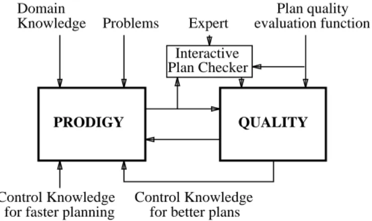
assumes that the planner’s domain theory is extended with an function that evaluates the quality of final produced plans. Learning consists in a translation task of the plan evaluation function into control knowledge usable by the planner at plan generation time. Figure 11 shows the architecture of

implemented within

PRODIGY

4.0.

Domain

Knowledge Problems Expert

Plan quality evaluation function

Control Knowledge for faster planning

Control Knowledge for better plans

PRODIGY QUALITY

Plan Checker Interactive

Figure 11: Architecture of the learning module

, to learn control knowledge to improve the quality of plans.

The learning algorithm is given a domain theory (operators and inference rules) and a domain-dependent function that evaluates the quality of the plans produced. It is also given problems to solve in that domain.

QUALITY

analyzes the problem-solving episodes by comparing the search trace for the planner solution given the current control knowledge, and another search trace corresponding to a better solution (better according to the evaluation function). The latter search trace is obtained by asking a human expert for a better solution and then producing a search trace that leads to that solution, or by letting the problem solver search further until a better solution is found. The algorithm explains why one solution is better than the other and outputs search control knowledge that directs future problem solving towards better quality plans.

Two points are worth mentioning:

Learning is driven by the existence of a better solution and a failure of the current control knowledge to produce it.

There is a change of representation from the knowledge about quality encoded in the domain- dependent plan evaluation function into knowledge operational at planning time, as the plan and search tree are only partially available when a decision has to be made. The translated knowledge is expressed as search-control knowledge in terms of the problem solving state and meta-state, or tail plan, such as which operators and bindings have been chosen to achieve the goals or which are the candidate goals to expand.

We do not claim that this control knowledge will necessarily guide the planner to find optimal solutions, but that the quality of the plans will incrementally improve with experience, as the planner sees new interesting problems in the domain.

4.2.1

: The Algorithm

Table 4 shows the basic procedure to learn quality-enhancing control knowledge, in the case that a human

expert provides a better plan. Steps 2, 3 and 4 correspond to the interactive plan checking module, that

asks the expert for a better solution

and checks for its correctness. Step 6 constructs a problem solving

trace from the expert solution and obtains decision points where control knowledge is needed, which in turn

become learning opportunities. Step 8 corresponds to the actual learning phase. It compares the plan trees

obtained from the problem solving traces in Step 7, explains why one solution was better than the other,

and builds new control knowledge. These steps are described now in detail.

1. Run

with the current set of control rules and obtain a solution . 2. Show

to the expert.

Expert provides new solution

possibly using

as a guide.

3. Test

. If it solves the problem, continue. Else go back to step 2.

4. Apply the plan quality evaluation function to

. If it is better than

, continue. Else go back to step 2.

5. Compute the partial order for

identifying the goal dependencies between plan steps.

6. Construct a problem solving trace corresponding to a solution

that satisfies .

This determines the set of decision points in the problem solving trace where control knowledge is missing.

7. Build the plan trees

and

, corresponding respectively to the search trees for

and

. 8. Compare

and

explaining why

is better than

, and build control rules.

Table 4: Top level procedure to learn quality-enhancing control knowledge.

Interactive plan checker

interacts with an expert to determine variations to the plan currently generated that may produce a plan of better quality. We have built an interactive plan checker to obtain a better plan from the domain expert and test whether that plan is correct and actually better. The purpose of the interactive plan checker is to capture the expert knowledge about how to generate better plans in order to learn quality-enhancing control knowledge. The interaction with the expert is at the level of plan steps, i.e. instantiated operators, and not of problem-solving time decisions, relieving the expert of understanding

PRODIGY

’s search procedure.

The plan checker offers the expert the plan obtained with the current knowledge as a guide to build a better plan. It is interactive as it asks for and checks one plan step at a time. The expert may pick an operator from the old plan, which is presented in menu form, or propose a totally new operator. There is an option also to see the current state. The plan checker verifies the correctness of the input operator name and of the variable bindings according to the type specifications and may suggest a default value if some is missing or wrong. If the operator is not applicable in the current state, the checker notifies the expert which precondition failed to be true. When the new plan is completed, if the goal is not satisfied in the final state, or the plan is worse than the previous plan according to the plan quality evaluation function, the plan checker informs and prompts the expert for another plan, as the focus is on learning control knowledge that actually improves solution quality.

As we mentioned, the interaction with the user is at the level of operators, which represent actions in the world. In domains with inference rules, they usually do not correspond semantically to actions in the world and are used only to compute the deductive closure of the current state. Therefore the plan checker does not require that the user specifies them as part of the plan, but it fires the rules needed in a similar way to the problem solver. A truth maintenance system keeps track of the rules that are fired, and when an operator is applied and the state changes, the effects of the inference rules whose preconditions are no longer true are undone.

Constructing a problem solving trace from the plan Once the expert has provided a good plan, the problem solver is called in order to generate a problem solving trace that corresponds to that plan. However we do not require that the solution be precisely the same. Because our plan quality evaluation functions are additive on the cost of operators, any linearization of the partial order corresponding to the expert solution has the same cost, and we are content with obtaining a trace for any of them. (Veloso, 1989) describes the algorithm that generates a partial order from a total order.

To force the problem solver to generate a given solution, we use

’s interrupt mechanism (Car-

bonell et al., 1992), which can run user-provided code at regular intervals during problem solving. At each decision node it checks whether the current alternative may be part of the desired solution and backtracks otherwise. For example, at a bindings node it checks whether the instantiated operator is part of the ex- pert’s plan, and if not it tries a different set of bindings. The result of this process is a search trace that produces the expert’s solution, and a set of decision points where the current control knowledge (or lack of it) was overridden to guide

towards the expert’s solution. Those are learning opportunities for our algorithm.

Building plan trees At this point, two problem solving traces are available, one using the current control knowledge, and other corresponding to the better plan.

builds a plan tree from each of them. The nodes of a plan tree are the goals, operators, and bindings, or instantiated operators, considered by

during problem solving in the successful search path that lead to that solution. In this tree, a goal is linked to the operator considered to achieve the goal, the operator is linked in turn to its particular instantiation, i.e.

bindings, chosen and the bindings are linked to the subgoals corresponding to the instantiated operator’s preconditions. Leaf nodes correspond to subgoals that were true when

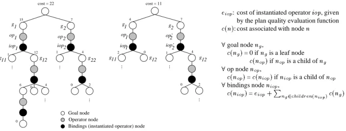
tried to achieve them. The reason for them being true is stored in the goal node: either they were true in the initial state, or were achieved by some operator that was chosen for other subgoal. Figure 12 shows the plan trees corresponding to two plans for the same problem.

Next the plan quality evaluation function is used to assign costs to the nodes of the plan tree, starting with the leaves and propagating them back up to the root. The leaf nodes have cost 0. An operator node has the cost given by the evaluation function, plus the sum of the costs of achieving its preconditions, i.e the costs of its children subgoals. Operator and bindings nodes have the same cost. A goal node has the cost of the operator used to achieve it, i.e. of its child. Note that if a goal had to be reachieved, it has more than one child operator. Then the cost of achieving the goal is the sum of the costs of the children operators. The root cost will be the cost of the plan. The plans for the plan trees in Figure 12 have different costs, with the tree on the left corresponding to the plan of worse quality. Note that the solutions differ in the operator and bindings chosen to achieve

. Those decisions are the ones for which the guidance provided by control knowledge is needed.

15 7

1 12

6

0

0 4

1 4

0 2

g1 op1 iop1

g11 g12

g2 op2 iop2

4 7

2 0 1 4

0 2

g1 op1 iop1

g11 g12

g2 op’2 iop’2

g12

cost = 22 cost = 11

g22

Goal node Operator node

Bindings (instantiated operator) node

: cost of instantiated operator , given by the plan quality evaluation function

: cost associated with node

goal node ,

= 0 if is a leaf node

if is a child of

op node ,

= if is a child of

bindings node ,

= ^"!#%$ &('*),+

-.0/1,2"3

Figure 12: Plan trees corresponding to two solutions of different quality for the same problem. The

cumulative cost of each subtree is propagated up to its ancestrors. A number next to a node indicates the

cost of the subtree rooted at that node.

Learning control rules Using the two plan trees, the algorithm explains why one solution is better than the other. The cost of the two plan trees is compared recursively, starting with the root, looking for cost differences. In the trees of Figure 12 the cost of achieving

is the same for both trees, but the cost of achieving

is different. Therefore

’s subtrees are explored in turn. The cost of the children operators is the same, as they are the same operators. However one of their subgoals,

, was less expensive to achieve in the better solution. In fact it had cost zero because it was shared with the subtree corresponding to

. The algorithm considers that this explains the different costs of the plans. Note that it ignores subgoals that had higher cost in the cheaper solution, such as

, therefore introducing incompleteness in the explanation construction.

This explanation, namely that

is shared, is made operational, i.e. expressed using knowledge avail- able to the planner at decision time. Step 6 in the algorithm (Table 4) indicated the learning opportunities, or wrong decisions made by the planner where new control knowledge was required.

with bindings corresponding to

should be preferred over

. This corresponds to an operator and bindings decision.

The explanation is propagated up the subtrees until it reaches the node corresponding to the decision point, gathering the conditions under which

is a shared subgoal. At that node

was a pending goal (a subgoal of

), and for

to be a shared subgoal, precisely

should be chosen with the appropriate set of bindings in

. With these facts the control rules are built. The learning opportunity defines the right-hand side of each rule, i.e. which operator or bindings to prefer, and some of the preconditions such as what the current goal is. The rest of the preconditions come from the explanation. The algorithm is also able to learn goal preferences.

4.2.2 Example: Plan Quality in the Process Planning Domain

To illustrate the algorithm just described, we introduce an example in the domain of process planning for production manufacturing. In this domain plan quality is crucial in order to minimize both resource consumption and execution time. The goal of process planning is to produce plans for machining parts given their specifications. Such planning requires taking into account both technological and economical considerations (Descotte and Latombe, 1985; Doyle, 1969), for instance: it may be advantageous to execute several cuts on the same machine with the same fixing to reduce the time spent setting up the work on the machines; or, if a hole

opens into another hole

, then one is recommended machining

before

in order to avoid the risk of damaging the drill. Most of these considerations are not pure constraints but only preferences when compromises are necessary. They often represent both the experience and the know-how of engineers, so they may differ from one company to the other.

Section 2 gave a (very) simplified example of the actions involved in drilling a hole. Here we use a much more realistic implementation of the domain in

(Gil, 1991; Gil and P´erez, 1994). This implementation concentrates on the machining, joining, and finishing steps of production manufacturing.

In order to perform an operation on a part, certain set-up actions are required as the part has to be secured to the machine table with a holding device in certain orientation, and in many cases the part has to be clean and without burrs from preceding operations. The appropriate tool has to be selected and installed in the machine as well. Table 5 shows the initial state and goal for a problem in this domain. The goal is to produce a part with a given height, namely , and with a spot hole on one of its sides, namely

. The system also knows about a domain-dependent function that evaluates the quality of the plans and is additive on the plan operators. If the right operations and tools to machine one or more parts are selected so portions of the set-ups may be shared, one may usually reduce the total plan cost. The plan quality metric used in this example captures the different cost of setting up parts and tools on the machines required to machine the part.

Assume that, with the current control knowledge, the planner obtains the solution in Table 6 (a)

')(*,+-./01./2%34)(*)-516789*%

4:(*,850687);&%<=43(*)>?0@78:;&%&AAA%%

B C(D"E+F7&%%3=G43C(D,8506873H%

I(JC(D,IKK3KLAM;N*,OPAQH*?%%%

Table 5: Example problem, showing the goal and a subset of the initial state.

that uses the drill press to make the spot hole. For example, the operation

indicates that

will be drilled in

on the drill press

using as a tool

, while the part is being held with its side 1 up, and sides 2 and 5 facing the holding device,

. This is not the only solution to the

(mnKJ(K

(mIBopJKqoK

p:(*

(mpInK"(*

I3KnoK"(*3K)H*

?I(qK"(Kro?K

(*,IKKJH*

(m"&BpI?Kr(&K

JKqoK(*

oIBopqKnoK

(mIBop2BpIKsoK

omn(*)mIK

p:(*

(mpIt&BpIKs(*

I)2BpIKsoK"(*:K;

p&t&BpI?Kr(*,(&KnoK

K); "IBI9H

p3u<Hv

(m,&BpIK(K

(mIBop"&BpIKsoK

p3(*

(mpI?t&BpIKs(*

I,&BpIKsoK(*:K);

I("&BpIK

(Kro?K"(*)IK)K);

o&BpIK(K

(m,&BpIKq(&K

p&t&BpIKs(*)(&K

oKJK; "IBI9H

p:u K*

(a) (b)

Table 6: (a) Plan obtained by

guided by the current control knowledge. (b) A better plan, according to the evaluation function, possibly input by a human expert.

problem. In this domain milling machines, but not drill presses, can be used both to reduce the size

of a part, and to drill holes and spot holes on it. Therefore there exists a better plan, according to

the evaluation function, that uses the milling machine to drill the spot hole, and shares the same set-up

(machine, holding device, and orientation) for the drill and mill operations, so that the part does not

have to be released and held again. These differences correspond at problem-solving time to an operator

decision (prefer

over

) and

an instantiation decision (bindings for

). Table 6 (b)

shows the improved plan. This plan may be input by a human expert using the interactive plan checker. The

search traces corresponding to plans (a) and (b) are transformed in plan trees, similar to the ones shown in

Figure 12. If the hole is drilled in the milling-machine using the proper holding device and orientation, the

subgoal

is shared by the face-mill and

drill operations. To explain that

with those particular bindings is shared, the algorithm traverses

the tree up from that goal node finding that

should be

chosen with the appropriate set of bindings, which includes using a machine of type milling machine and

a particular holding device and orientation. Note that the machine type determines not only the bindings