The Welfare Effects of Slum Improvement Programs

The Welfare Effects of Slum Improvement Programs

The Case of Mumbai

Akie Takeuchi (University of Maryland)

Maureen Cropper (World Bank)

Antonio Bento (University of Maryland)

World Bank Policy Research Working Paper 3852, February 2006

The Policy Research Working Paper Series disseminates the findings of work in progress to encourage the exchange of ideas about development issues. An objective of the series is to get the findings out quickly, even if the presentations are less than fully polished. The papers carry the names of the authors and should be cited accordingly. The findings, interpretations, and conclusions expressed in this paper are entirely those of the authors. They do not necessarily represent the view of the World Bank, its Executive Directors, or the countries they represent. Policy Research Working Papers are available online at http://econ.worldbank.org.

We thank Judy Baker, Rakhi Basu, and Somik Lall (World Bank) for their contribution in data collection and the World Bank TUDTR for funding the study.

WPS3852

Public Disclosure AuthorizedPublic Disclosure AuthorizedPublic Disclosure AuthorizedPublic Disclosure Authorized

The Welfare Effects of Slum Improvement Programs: The Case of Mumbai

I. Introduction

Slums, which are characterized by substandard housing and inadequate water and sanitation facilities, are among the most pressing urban environmental problems in developing countries. Policies to improve the welfare of slum dwellers include upgrading slum housing in situ—for example, by providing piped water and sewage connections—and relocating slum dwellers to better quality, low cost housing.

The goal of this paper is to evaluate the welfare effects of such programs using data for Mumbai (Bombay), India. A key issue in slum upgrading is whether current residents are made better off by improving housing in situ, or by relocating. The answer to this question depends on the tradeoffs people are willing to make between commuting costs, housing costs and the attributes of the housing that they consume. If, for example, a relocation program distances a worker from his job and, if finding a new job is difficult, in situ improvements in housing may dominate relocation programs. The utility of relocation programs also depends on neighborhood composition: if households depend on neighbors of the same caste or ethnic group for information about employment or for social services, relocation to neighborhoods of different ethnicity may be welfare- reducing.

Evaluating the welfare effects of slum upgrading and resettlement programs

requires estimating models of residential location choice, in which households trade off

commuting costs against the cost and attributes of the housing they consume, including

neighborhood attributes. We accomplish this using data for 5,000 households in Mumbai,

a city in which 40% of the population lives in slums. A key feature of Mumbai that distinguishes it from other Third World cities is that many slums are centrally located, i.e., located near employment centers, rather than being relegated to the periphery of the city.

Slum relocation projects may therefore involve moving people to more remote locations.

We ask what corresponding improvements in housing and/or income would be necessary to offset the location change.

To answer these questions we estimate a model of residential location choice for households in Mumbai. The choice of residential location is modeled as a discrete choice problem in which each household’s choice set consists of the chosen house plus a random sample of 99 houses from the subset of the 5,000 houses in our sample that the household can afford. Houses are described by a vector of housing characteristics and by the

characteristics of the neighborhood within a 1 km radius of the house. Two important neighborhood characteristics are ethnic composition (the percent of one’s neighbors of the same religion and same mother tongue) and employment accessibility. In one specification we treat the employment location of the primary household earner as fixed and characterize houses by their distance from the current work location. In an alternate specification we replace distance to the current workplace by an employment

accessibility index, to capture opportunities for changing jobs.

We use the model of residential location to examine the welfare effects of specific

programs—in situ improvements in housing attributes and the provision of basic public

services, and a slum relocation program. Historically, both types of programs have been

implemented in Mumbai (Mukhija 2001; Mukhija 2002). In 1985 the World Bank

launched the Bombay Urban Development Project to provide tenure security and

encourage in situ upgrading by slum dwellers. In the same year the Prime Minister’s Grant Project (PMGP), introduced by the state of Maharashtra, proposed to construct new housing units on the sites of existing slums in Dharavi. Currently the Valmiki Ambedkar Awas Tojana Program (VAMBAY) provides loans to the poor to build or upgrade

houses.

The economics literature on the benefits of slum improvements has, for the most part, consisted of hedonic studies that estimate the market value of various improvements, including tenure security and infrastructure services (Crane et al. 1997; Jimenez 1983, 1984). Kaufman and Quigley (1987) advanced this literature by estimating the

parameters of household utility functions rather than limiting the analysis to the hedonic price function. We extend this literature in three ways: first, we introduce employment access as a factor influencing the choice of residential location; secondly, we incorporate endogenous neighborhood amenities—in particular, the language and religion of one’s neighbors—in residential location choice; thirdly, we account for unobserved

heterogeneity in housing and neighborhood attributes, in the spirit of Bayer et al. (2004b).

The paper is organized as follows. Section 2 describes the data used in our empirical work and presents the stylized facts about where people live and work in Mumbai. Section 3 describes the model of residential location choice. Section 4 presents estimation results and section 5 the welfare effects of slum upgrading policies. Section 6 concludes.

1 http://mhada.bom.nic.in/html/web_VAMBAY.htm

II. Job and Housing Locations in Mumbai

The target population of our study is households in the Greater Mumbai Region (GMR), which constitutes the core of the Mumbai metropolitan area. The GMR, with a population of 11.9 million people in 2001, is one of the most densely populated cities in the world. Located on the Arabian Sea, the GMR extends 42 km north to south and has a maximum width of 17 km. The Municipal Corporation of Greater Mumbai has divided the city into 6 zones (see Figure 1), each with distinctive characteristics. The southern tip of the city (zone 1) is the traditional city center. Zone 3 is a newly developed commercial and employment center, and zones 4, 5 and 6, each served by a different railway line, constitute the suburban area. In the remainder of this section we describe the distribution of population and jobs in the GMR, as well as the characteristics of the housing stock, based on a random sample of 5,000 households in Mumbai who were surveyed in the winter of 2003-2004 (Baker et al. 2005).

Table 1 presents our sample households, broken down by income category.

Households earning 5,000 Rs. per month or less constitute the bottom quartile (26.5%) of our sample, households earning 5,000-7,500 Rs. per month the next quartile (27.7%), households earning 7,500-10,000 Rs. per month 22% of our sample, and households in the next two income categories 18% and 6% of our sample, respectively.

Almost 40% of our sample households live in slums, with the percent living in slums increasing as income falls. This number is consistent with the extent of slums in other cities (United Nations Global Report on Human Settlements 2003). According to the United Nations, 924 million people, or 31.6% of the world’s urban population, lived

2 In PPP terms, 5,000 Rs. corresponds to $562 USD.

in slums in 2001. Slums in Mumbai were formed by residents squatting on open land as the city developed.

Slum residents do not possess a transferable title to their property;

however, “notified” squatter settlements have been registered by the city, and slum dwellers in these settlements are unlikely to be evicted.

Chawls, which house approximately 35% of sample households, are usually low-rise apartments with community toilets that, on average, have better amenities than slums. The remaining 25% of households live either in cooperative housing, which includes modern, high-rise apartments, in bungalows, or in employer-provided housing.

A. Distribution of Population and Housing

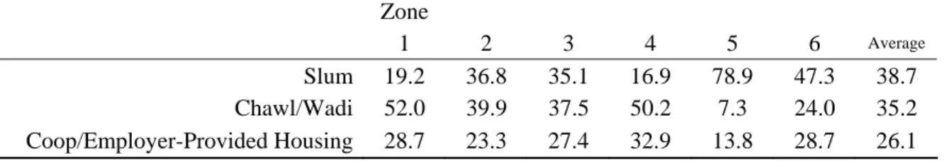
The spatial distribution of sample households by housing type is shown in Figures 2 and 3, where each dot represents 5 households, and is summarized in Table 2. Slums are not evenly spread throughout the city: they constitute a higher-than-average fraction of the housing stock in zones 5 and 6 (79% and 47%, respectively), but less than 20% of the housing stock in zones 1 and 4. Nonetheless, slum dwellers in Mumbai are

considerably more integrated among non-slum dwellers than in other cities: 40% of slum- dwellers live in central Mumbai (zones 1-3).

In contrast, there are virtually no slums in central locations in Delhi or many cities in Latin America (United Nations Global Report on Human Settlements 2003). In these cities, slums are typically located at the periphery:

as a consequence, slum dwellers may spend several hours commuting to work.

3 For example, Dharavi, the world’s largest slum, was originally a fishing village located on swamp land.

Slums began forming there in the late 19^th century when land was reclaimed for tanneries. Once on the periphery of Mumbai, Dharavi is now centrally located (in zone 2).

41.8 % of our sample households live in “non-notified” slums and 1.6 % in resettlement areas. The average tenure of households in notified squatter settlements suggests that squatters are unlikely to be evicted: 81%

of households have been living in current location for more than 10 years while corresponding figure for the formal housing sector is 74%.

5 This is also true of the poor v. the non-poor. See Baker et al. (2005) Figure 2 and Tables 2 and 3.

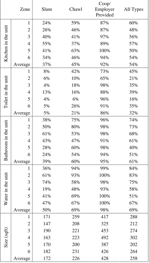
Table 3 shows characteristics of the housing stock by housing type and zone. It attests to the fact that slum dwellings are, on average, smaller than either chawls or cooperative housing, and less likely to have piped water connections or a kitchen inside the dwelling. It is, however, clear that the quality of slum housing varies considerably by zone: whereas 61% of slum households have piped water in zone 2, only 19% of slum households have piped water in zone 4.

B. Distribution of Jobs and Commuting Patterns

Table 4, based on data for 6,371 workers in our sample households, shows where people living in each zone work.

Fifty-seven percent of workers in our sample

households work in zones 1-3, 31% in the suburbs (zones 4-6), and 6% at home. The rest either do not work in a fixed location or work outside of the GMR. A striking feature of Table 4 is the high percent of workers who live in the same zone in which they work.

This is highest in zones 1-3, but is substantial even in the suburbs. Replicating Table 4 for different income and occupational groups reveals that the diagonal elements in the table (the percent of people working and living in the same zone) are higher for workers in low-income than in high-income households, and are higher for unskilled and skilled laborers than for professionals (Baker et al. 2005, Tables 38 and D-1).

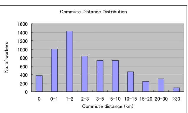
Figure 4, which shows the distribution of one-way commute distances for workers in our sample is consistent with Table 4: the median journey to work is less than 3

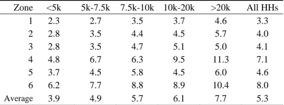
kilometers, although the distribution of commute distances has a long tail. Table 5, which shows mean commute distance by zone and income, suggests that persons with longer commutes are more likely to live in the suburbs, especially in zones 4 and 6. With

6 Table 4 is based on the usual commutes of the two most important earners in each household. Forty percent of sample households have more than one earner.

few exceptions, mean commute to work increases with income, regardless of zone of residence.

The information presented here suggests that, on average, people in Mumbai live close to where they work: This is especially true for the poor, and also for laborers. This suggests that households may place a high premium on short commutes. If, in the short run, workers’ job locations are fixed, slum upgrading programs that require households to move may reduce welfare if they move workers farther from their jobs. The impact of such programs on welfare will, however, also depend on the value attached to housing and neighborhood amenities.

III. Analytical Framework

The models of residential location choice we have estimated are descendants of discrete location choice models (e.g., McFadden 1978), but incorporate the recent

literature on the treatment of unobserved heterogeneity in discrete location choice models (Bayer et al. 2004b). This section describes in detail the structure of these models and how they will be used to evaluate slum improvement programs.

A. Modeling Location Choice

We assume that the utility that household i receives from house h depends on a vector X

of house characteristics, a vector Z

of aggregate household characteristics of the neighborhood the house belongs to (e.g., ethnic composition) and on an index of employment accessibility for the principal earner in the household, E

. Utility also depends on expenditure on all other goods, i.e., on income y

minus the user cost of housing, p

. Formally,

ih h h i h p

i h E

Z h h X

i

X Z E y p

U = β + β + β + β ln( − ) + ξ + ε (1)

where

β

= α

+α

Z

r=X, Z,E, p. (2)

In (1) ξ

is a house specific constant that captures unobserved house and neighborhood characteristics that are perceived identically by all households; ε

captures unobserved housing characteristics as perceived by household i. Equation (2) allows each element j of the β coefficient vectors to depend on the inner product of a vector of household characteristics, Z

, and a vector of coefficients α

.

Estimation of the parameters of (1) and (2) will allow us to infer the rate of

substitution between accessibility to work and housing cost, and accessibility to work and neighborhood and housing characteristics. To evaluate the welfare effect of moving household i from its chosen location to a new one, we compute the amount, CV, that must be added to the Hicksian bundle to keep the systematic part of the household’s utility constant when it is moved.

C. Estimation of the Model

In estimating the model of residential location choice each household’s choice set consists of the chosen house plus a random sample of 99 houses from the subset of the 4,023 houses in our sample that the household can afford.

Because the housing attributes in our dataset are highly correlated, we use principal components of the attributes in estimating the parameters of equation (1).

Estimation of the parameters of (1) follows the two-step approach outlined in Bayer et al. (2004b). Let δ

represent the portion of (1) that varies only by house, i.e.,

7 CV is negative for a net improvement in housing and neighborhood characteristics.

8 The original set of approximately 5,000 households is reduced because information about housing characteristics is missing for some houses, and because we eliminate employed-provided housing from the choice set.

α

X

+ ξ

, and θ the vector of parameters on variables in (1) that vary by both

household and house (ln(y

-p

), and the interaction of housing and neighborhood attributes with household characteristics).

ih

E

9

We find the vector θ that maximizes the likelihood function for a given value of {δ

} and calculate the estimated demand for each house h as

∑

=

i ih

h

P

D .

In the second step, we search for the set of {δ

} that satisfy the maximization condition in equation (3), given our first-stage estimate of θ,

0 1

) 1 ( /

ln ∂ = − + = − =

∂ ∑ ∑

≠ i

ih h

i ih hh

h

P P P

L δ

∀ h . (3)

Berry (1994) and Berry, Levinsohn, and Pakes (1995) show that for any θ the unique {δ

} that satisfy above conditions can be obtained by solving the contraction mapping

)

1

^{= −} ln( ∑

+

i ih t

h t

h

δ P

δ (4)

The {δ

} obtained in the second stage are used to re-estimate θ in step one. The procedure is iterated until our estimators converge. δ

is then regressed on X

to determine the coefficient vector α

.

IV. Estimation Results

A. Specification of the Utility Function

We assume that a household’s utility from its residential location [eq. (1)]

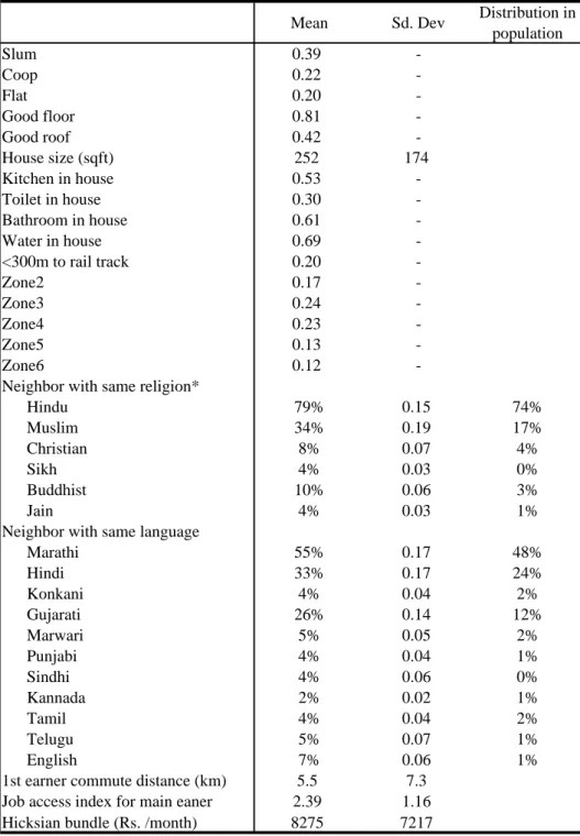
depends on housing and neighborhood characteristics. The first ten variables in Table 6 describe the house itself: whether the dwelling is a slum or a cooperative (chawl is the

9 The neighborhood characteristics used in our empirical work include religion and native language. We assume that α0Z = 0.

omitted category), whether it is a multi-story dwelling (flat), dummy variables to indicate the quality of the floor and roof, and the interior space in square feet. This is followed by a series of dummy variables indicating whether the house has a kitchen, a toilet, or a bathroom (i.e., a room for washing), and whether there is a piped water connection in the house. Due to the high correlation among these housing characteristics we replace them in empirical work by their first two principal components, which have eigenvalues

greater than one.

We characterize the location of the house in terms of its distance from the nearest railroad track (whether it is < 300m from a track) and by the zone in which it is located.

Neighborhood characteristics Z

include religion and mother tongue.

Specifically, we assume that utility is a function of the percent of households in the neighborhood that (a) are of the same religion as the household in question and (b) who speak the same mother tongue.

These variables should capture network externalities and other forms of social capital provided by neighbors of the same ethnic background.

Table 6 indicates the degree of ethnic sorting in Mumbai: For example, while Muslim households comprise only 17% of the city’s population, the average Muslin household in our sample lives in a neighborhood that is 35% Muslim. Although people from the state of Gujarat constitute only 12% of the population of Mumbai, the average household from Gujarat in our sample lives in a neighborhood that is 26% Gujarati. The extent of ethnic sorting is greater, in relative terms, for minority groups—e.g., for Sikhs, Christians,

10 The first two principal components explain approximately 60% of the variance in housing attributes.

11 The results in Tables 7 and 9 change little if zone dummies are replaced by section dummies. (There are 88 sections in Mumbai.) We report results using zone dummies for ease of interpretation.

12 Neighborhood characteristics are computed using sample households within 1 km of each house. A neighborhood contains, on average, 67 sample households, although the number varies depending on the population density of the area.

Buddhists, Tamils and Telugus—than for households in the majority (i.e., Hindus or households that speak Marathi or Hindi). For this reason we allow the coefficient on ethnic composition to vary with the percent of one’s neighbors from the same

background.

Employment access (E

) for the principal wage earner in the household is computed as follows. In Model 1, access is measured by the distance from house h to the worker’s current job location.

The weight attached to distance from the current job location should capture the disutility of relocating in the short run, before the worker can change jobs. In Model 2, we replace distance to the current job from house h by the average distance from house h to the 100 nearest jobs in the worker’s occupation, based on our survey data. We distinguish five occupations in computing the employment accessibility index: unskilled workers, skilled workers, sales and clerical workers, small business owners, and managers/professionals. This variable should capture the disutility of being moved away from desirable employment locations, even if the worker can change jobs.

Utility also depends on the log of monthly household income minus the cost of housing (i.e., the log of the Hicksian bundle). The Hicksian bundle is calculated as follows. All sample households were asked what “a dwelling like theirs” would rent for and what it would sell for.

We use the stated monthly market rent as the cost of the

13 The distance from house h to a worker’s job is estimated as the distance between house h (whose location is geo-reference in the survey) and the approximate work location. The work location is approximated by the centroid of the intersection of the section and pin code in which the job is located.

14 We have used the answers to these questions to compute for each household the interest rate that would equate the purchase price of the house to the discounted present value of rental payments. The mean interest rate is 5.6% and the median 4.8%. Additional evidence that stated market rents are reliable is provided by using them to estimate an hedonic price function for housing in Mumbai. The housing and neighborhood characteristics in Table 6, together with distance to the CBD, explain 64% of the variation in monthly rents in our sample. (See Table A1.)

dwelling. In calculating the income of households who currently own their home, we add to household income from earnings and other sources the monthly rent associated with the dwelling they own. For renters, household income is stated income from earnings and other sources.

The mean value of the Hicksian bundle, evaluated at the current residence, is 8,275 Rs. The median Hicksian bundle approximately 6,250 Rs. per month.

B. Results

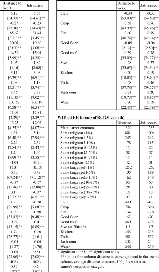
Table 7 presents the results of estimating our models. The first column of the table presents estimates of the parameter vectors θ and α

. The parameter vector θ, which contains the coefficients of all variables that vary by household (i.e., the Hicksian bundle through measures of language and religion) is estimated in the first stage of the estimation procedure together with the set of house-specific constants {δ

}. In the second stage, the {δ

} are regressed on the principal components of housing

characteristics, as well as the zone dummies and whether the house is within 300 m of a railroad track. The second column of the table presents the coefficients of the individual housing attributes, as well as the marginal value of each amenity, i.e., the marginal rate of substitution between the amenity and the Hicksian bundle, evaluated at the median

household income for our sample (6,250 Rs. per month).

In both specifications all housing attributes are statistically significant at the 5%

level. Other things equal, being in a chawl (the omitted housing category), is worth about 400 Rs. per month more than being in a slum, whereas being in a coop is worth about 700 Rs. more than being in a chawl. Being in a high-rise building (flat) is worth about 730 Rs.

per month. The mean value of a piped water connection is about 240 Rs. per month, and

15 Seventy-four percent of sample households claim to own their own home, whereas 26% indicate that they rent. Surprisingly, 83% of households living in notified squatter settlements claim to own their own homes, although it is unlikely that they possess a transferable title.

mean willingness to pay for a private toilet about 580 Rs. per month. Overall, the value attached to housing attributes seems reasonable, with the exception of “good floor.”

Workers in Mumbai place a premium on living close to where they work. Model 1 suggests that a household with income of 6,250 Rs. per month would give up about 330 Rs. to decrease the main earner’s one-way commute by 1 km.

In Model 2, the value of a one km decrease in the average distance to the 100 nearest jobs in one’s occupation is 283 Rs.

Neighborhood attributes matter. The value of being with households who speak the same mother tongue and have the same religion depends on whether one is in the minority or the majority. In a neighborhood where only 5-10% of one’s neighbors speak the same mother tongue, the value of a one percentage point increase in mother tongue is large (162 Rs.). [All values refer to model 1.] In a neighborhood where 50-75% of one’s neighbors speak the same mother tongue, the value of a one percentage point increase is only 15 Rs. Similar results hold for living with members of the same religion: a one percentage point increase in the percent of households of the same religion is worth 178 Rs. evaluated at a baseline of 5-10% but is worth only 13 Rs. in a neighborhood where 50-75% of households are already of the same religion.

These values are large, and may reflect various forms of network externalities.

Munshi and Rosenzweig (2004) emphasize the importance of networks, formed along caste lines, in determining the jobs available to workers in Mumbai. These networks are especially important for laborers and unskilled workers. Similarly, in the United States, Bayer, Ross and Topa (2004) find significant evidence of informal hiring networks, based

16 When the distance of the second main earner’s commute is included in the model, the value of a one km decrease in the second earner’s commute is about 300 Rs. per month.

on the fact that individuals residing in the same block group are more likely to work together than those in nearby but not identical blocks.

In addition to providing employment networks, neighborhoods also serve as social capital to mitigate the effects of poverty. For example, social networks make possible the creation of spontaneous mechanisms of informal insurance and can improve the efficiency of public service delivery and/or of public social protection systems (Collier 1998).

We should, however, be cautious in interpreting these effects. In reality it is virtually impossible to disentangle the different reasons why similar individuals live in the same neighborhood.

Part of this sorting is indeed due to preferences. However, neighborhood composition could also be a result of imperfections in housing markets that segregate individuals to specific neighborhoods.

Other amenities that affect residential location are proximity to a railroad track as well as the zone dummies. Living next to a railroad track can be dangerous, in addition to providing visual disamenities: Approximately 6 people are killed each day crossing railroad tracks in Mumbai. The impact of zone dummies varies with the measure of employment access.

V. Evaluating Slum Improvement Programs

The set of policies that have been employed to improve the welfare of slum dwellers is diverse (Field and Kremer 2005, Mukhija 2001). Some projects have focused on providing secure tenure, on the grounds that this will provide an incentive for slum

17 Ethnic sorting does not appear to reflect the fact that people of the same religion or mother tongue have common educations and incomes. When we attempt to use income and education to explain variation in the exposure of households in minority groups to members of their group, F statistics are rarely significant.

dwellers to invest in housing (Jimenez 1983, 1984; Malpezzi and Mayo 1987). Other projects, such as those implemented under the World Bank’s Sites-and-Services program (Kaufmann and Quigley 1987; Buckley and Kalarickel 2004) have combined secure tenure with provision of basic infrastructure services (piped water and electricity) and loans to allow slum dwellers to themselves build/upgrade their housing.

More recently, greater emphasis has been placed on providing incentives for community management and maintenance, including constructing or rehabilitating community centers, and on improving access to health care and education.

In this paper we focus on improving the physical aspect of slums by providing infrastructure services and improving housing quality. In Mumbai, virtually all slum dwellers have access to electricity; however, only half have piped water. Slum housing consists of small, dilapidated shacks with poor roofs. Programs to improve the physical quality of housing could involve in situ improvements or could involve housing

reconstruction, either at the site of the original slum or in a location where bare land is available.

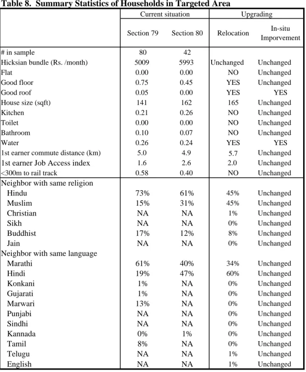
We evaluate stylized versions of both types of programs—in situ upgrading and relocation of slum households to better housing. We focus on slum households located in zone 5, specifically households in sections 79 and 80 who are located within one mile of the Harbor Railway. The characteristics of our sample households living in these slums appear in Table 8. These households are, on average, much poorer than our sample as whole, although 85% claim to own their own home. Average house size is small—141

18 In the World Bank sites-and-services project in El Salvador evaluated by Kaufman and Quigley (1987), slum dwellers were given financing to purchase lots on which infrastructure services were provided, as well as materials to construct new homes. Imperfections in credit markets and in the provision of infrastructure services are major reasons for initiating slum improvement projects.

sq. ft. in section 79 and 162 sq. ft. in section 80. Almost no houses have good roofs and only one quarter have piped water connections. The primary earner in households in both sections commutes, on average, 5 km to work (one-way), although the variance in

commute distance is large. In terms of language and religion, the majority of households in section 79 are Marathi-speaking Hindus. In section 80, the majority of households speak Hindi; sixty percent are Hindus and one-third are Muslims.

The in situ program provides good roofs and piped water connections for

households that do not have them. The relocation program moves households from their current locations to new housing in Mankurd, a neighborhood in zone 5 where some households displaced by transportation improvement programs have been relocated.

(The original locations of households and the relocation site are shown in Figure 5.) We assume that households are moved into good quality, low-rise buildings with piped water but with community toilets. We assume in the short run that workers in resettled

households continue to work in their old job locations. The religious makeup of the new neighborhood is approximately half Hindu and half Muslim. Sixty percent of households speak Hindi and one-third speak Marathi.

To compute the welfare effects of each program, we calculate for each household the amount of money the household must be given, in exchange for the vector of program attributes, to keep the systematic portion of the household’s utility constant.

Compensating variation (CV) is implicitly defined as:

19 The second Mumbai Urban Transportation Program (MUTPII) will involve resettling 20,000 households located on railway rights-of-way.

)

ln(

0 0

0

Z E y p

X

X

+ β + β + β −

β = β

X

+ β

Z

+ β

E

+ β

ln( y

− p

+ CV )

where

’s denote housing and neighborhood attributes originally consumed and

’s denote attributes consumed with the program. Welfare effects from the relocation program are computed assuming that households pay the same amount for their housing with and without the program. CV should therefore be interpreted as the monetary value of the benefits of the program over and above current housing costs. Welfare effects from the relocation program are computed holding current job location fixed, to capture the short-run effects of the program and replacing current job location by the employment access index, to capture opportunities for workers to change jobs.

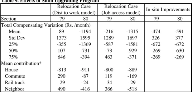
Table 9 reports the mean welfare effects of the in situ upgrading program and the relocation program under alternate assumptions about workplace location. The 25

, 50

and 75

percentile of CV values for the households in Table 8 are also presented in the table. The in situ upgrading program is worth, on average, approximately 500 Rs. per month, or about 10% of household income. The range of CV values for the programs reflects the range of incomes of the affected households. The mean benefit of the relocation program differs substantially between households who originally lived in section 79 and those who lived in section 80 and depends crucially on employment and neighborhood effects: Households originally residing in section 80 are, on average, better off under the relocation program than under in situ upgrading; the reverse holds for households from section 79.

20 This definition implies that CV is negative for a welfare improvement.

To better understand the impacts of relocating, Table 9 presents the mean effects of different components of the slum upgrading program. For example, the mean benefit of the housing improvement associated with the program is 813 Rs. per month for

households from section 79 (Distance to work model). Holding workplace location fixed, the mean disbenefit of being moved farther from the workplace is 290 Rs. per month, and the mean disbenefit of changing neighborhood composition 490 Rs. per month.

Although the relocation program yields approximately equal housing benefits to both groups, and moves households away from railroad tracks, workers from section 79 are being moved much farther from their jobs than workers who originally lived in section 80.

(The latter, on average, actually benefit by being moved closer to their jobs.) The other major difference in welfare between the two groups comes from neighborhood effects.

Households who originally lived in section 79, who are primarily Marathi-speaking Hindus, are being moved into a neighborhood with a greater proportion of Muslim and Hindi-speaking households. They lose, on average, from the change in neighborhood composition. For households from section 79, the disbenefits of changes in commute distance and neighborhood composition actually wipe out the housing benefits of the slum improvement program, a result consistent with Kapoor et al. (2004).

The impact of the relocation program however depends on the assumptions made about workplace location. When workplace location is held fixed, the households from section 79, who are on average being moved farther away from their jobs, are worse off than if they are able to change jobs: average welfare losses due to a longer commute go down when distance to work is replaced by the employment accessibility index (job

21 The sum of the mean compensating variations for each component of the program will not add to the mean CV for the program as a whole because the Hicksian bundle enters the utility function non-linearly.

access model). In the particular example illustrated in Table 9, however, the welfare impact of allowing workers to change jobs is not large in quantitative terms. This is because the site of improved housing is not far away from section 79.

Figures 6 and 7 illustrate more clearly the impact of changes in neighborhood composition and employment access on the benefits of slum improvement programs.

The figures plot the median CV associated with our sample improvement program, for all beneficiaries in Table 8, as the location of the improved housing is moved to different places in the city. In Figure 7 we assume that the primary worker in the household maintains his current place of employment when the household relocates; in Figure 6 we measure employment opportunities by the primary worker’s employment index. In both figures, blue areas indicate locations that are welfare-reducing; orange and yellow areas indicate moves that are, on average welfare-enhancing. (In both figures, neighborhood composition changes ipso facto with location.)

When each worker’s job location is held fixed (Figure 7), the set of locations for the program that yield positive benefits (negative mean CV) is small indeed. The set of locations yielding positive benefits is much larger in Figure 6, in which household utility depends on the employment access index. If potential participants in slum relocation programs look only at these programs from a short-run perspective (assuming that they cannot or will not change jobs), participation is likely to be much lower than if a longer- run perspective is taken.

VI. Conclusions

In the early Twentieth Century, slum improvement programs in many countries

were equivalent to slum clearance—hardly a solution to the problem of lack of adequate

housing in developing country cities. Beginning in the 1970’s the strategy shifted to one of improving and consolidating existing housing—often by providing slum dwellers tenure security, combined with the materials needed to upgrade their housing or—in areas where land was plentiful—to build new housing. Emphasis on in situ

improvements has continued to the present. These improvements may take the form of providing infrastructure services and other forms of physical capital, but also include efforts to foster community management, and access to health care and education. At the same time, some have called for replacing slums with multiple story housing either at the site of the original slum or in an alternate location.

In order to design successful slum improvement programs it is important to determine whether program benefits exceed program costs. It is also important, from the perspective of cost recovery, to determine household willingness to pay for specific program options. The early literature (Mayo and Gross 1987) focused on estimating the percent of income households were willing to spend on housing. This was followed by a literature that attempted to measure, using hedonic price functions, the market value of various improvements, including tenure security and infrastructure services (Crane et al.

1997; Jimenez 1984). It is, however, difficult using the hedonic approach to value attributes that vary by household, such as distance to work, or the percent of neighbors similar to oneself. We believe that both sets of attributes are important in valuing slum improvement programs and have attempted to extend the literature by illustrating the value placed on these amenities by households in Mumbai.

We believe that the model estimated in this paper can be of use in calculating the

relative welfare gains from alternative slum improvement programs. It is also useful in

predicting which households would be likely to participate in various programs, given

costs of participation. In assessing the limited success of sites-and-services programs,

Mayo and Gross (1987) cite the failure of many programs to choose the right package of

services to promote cost-recovery. Location is an important component of the design of a

slum improvement program. One contribution of this paper is to quantify, for the case of

Mumbai, the quantitative importance of location versus other program characteristics.

References

Baker, Judy, Rakhi Basu, Maureen Cropper, Somik Lall and Akie Takeuchi. 2005.

“Urban Poverty and Transport: The Case of Mumbai.” World Bank Working Paper, March 2005.

Bayer, Patrick, Robert McMillan and Kim S. Rueben. 2004a. “What Drives Racial Segregation? New Evidence using Census Microdata,” Journal of Urban Economics 56:

514-535.

Bayer, Patrick, Robert McMillan and Kim Rueben. 2004b. “An Equilibrium Model of Sorting in an Urban Housing Market.” NBER Working Paper Series No. 10865.

Cambridge, MA.

Bayer, Patrick, Stephen Ross and Giorgio Topa. 2004. “Place of Work and Place of Residence: Informal Hiring Networks and Labor Markets Outcomes.” Mimeograph. Yale University.

Berry, Stephen. 1994. “Estimating Discrete-Choice Models of Product Differentiation,”

RAND Journal of Economics 25: 242-262.

Berry, Stephen, James Levinsohn and Ariel Pakes. 1995. “Automobile Prices in Market Equilibrium,” Econometrica 63: 841-890.

Buckley, Robert and Jerry Kalarickal. 2004. “Shelter Strategies for Urban Poor:

Idiosyncratic and Successful, but Hardly Mysterious.” World Bank Policy Research Working Paper 3427.

Collier, Paul. 1998. “Social Capital and Poverty.” Social Capital Initiative Working Paper No. 4. World Bank.

Crane, Randall, Armita Daniere and Stacy Harwood. 1997. “The Contribution of Environmental Amenities to Low-Income Housing: A Comparative Study of Bangkok and Jakarta.” Urban Studies 34(9): 1495-1512.

Field, Erica and Michael Kremer. 2005. “Impact Evaluation for Slum Upgrading Interventions.” Mimeograph. Harvard University.

Global Report on Human Settlements. 2003. The Challenge of Slums. United Nations Human Settlements Program. Earthcan Publications Ltd., London, UK

Jimenez, Emmanuel. 1983. “The Magnitude and Determinants of Home Improvement in

Self-Help Housing: Manila’s Tondo Project.” Land Economics 59(1): 70-83.

Jimenez, Emmanuel. 1984. “Tenure Security and Urban Squatting.” The Review of Economics and Statistics 66(4): 556-567.

Kapoor, Mudit, Somik Lall, Mattias Lundberg and Zmarak Shalizi. 2004. “Location and Welfare in Cities: Impacts of Policy Interventions on the Urban Poor.” The World Bank.

Policy Research Working Paper 3318.

Kaufmann, Daniel, and John M. Quigley. 1987. “The Consumption Benefits of Investment in Infrastructure: The Evaluation of Sites-and-Services Programs in Underdeveloped Countries.” Journal of Development Economics 25(2): 263-284.

Kumar, A. 1991. “Delivery and Management of Basic Services to the Urban Poor: the Role of the Urban Basic Services, Delhi.” Community Development Journal 26(1): 50-60.

McFadden, Daniel. 1978. “Modeling the Choice of Residential Location,” in A.

Karlqvist, L. Lundquist, F. Snickars and J. Weibull (eds.), Spatial Interaction Theory and Planning Models, Amsterdam, North Holland.

Malpezzi, Stephen and Stephen Mayo. 1987. “User Cost and Housing Tenure in Developing Countries.” Journal of Development Economics 25: 197-220.

Mayo, Stephen K. and David J. Gross. 1987. “Sites and Services—and Subsidies: The Economics of Low-Cost Housing in Developing Countries.” World Bank Economic Review 1:301-335.

Mukhija, Vinit. 2001. “Upgrading Housing Settlements in Developing Countries: The Impact of Existing Physical Conditions.” Cities 18(4): 213-222.

Mukhija, Vinit. 2002.”An Analytical Framework for Urban Upgrading: Property Rights, Property Values and Physical Attributes.” Habitat International 26: 553-570.

Munshi, Kaivan and Mark Rosenzweig, 2004. Traditional Institutions Meet the Modern

World: Caste, Gender and Schooling Choice in a Globalizing Economy. Mimeo. Brown

University.

Table 1. Selected Household Characteristics in Mumbai, by Income Group Income Group (in rupees per month)

Characteristic < 5 k 5–7.5k 7.5–10k 10–20 k >20 k

Household size (mean) 4 4.4 4.6 4.6 4.4 4.4

Age of Head (mean) 38.2 39.4 41.1 42.9 45 40.4

Female Head (%) 8.8 3 3.9 3.2 1.3 4.5

Education (%)

Primary or less 20.6 10.8 7.2 2.0 0.3 10.4

College or above 4.0 7.9 17.0 39.2 66.5 18.0

Occupation (%)

Unskilled 33.9 21.0 11.1 3.5 1.3 17.9

Housing Category (%)

Squatter settlement 52.2 45.3 34.3 16.1 6.2 37.2

Chawls 37.5 37.5 41.5 27.6 9.9 34.9

Cooperative Housing 5.2 9.6 17.1 47.6 78 21

Other 5.1 7.7 7.2 8.8 5.9 7.1

Housing Tenure (%)

Less than 5 years 18.6 14.5 13.2 20.1 17.4 16.4

6-9 years 8.2 7.5 7.1 8.5 10.8 8

More than 10 years 34.5 35.3 34.7 31.3 46.6 35

Since birth 38.7 42.7 45 40.1 25.3 40.6

Within-household access to:

Piped Water 48 64 75 92 99 69

Toilet 12 18 31 64 89 32

Kitchen 29 43 61 87 98 54

Table 2. Percent of Households in Different Types of Housing by Zone

1 2 3 4 5 6 ^Average

Slum 19.2 36.8 35.1 16.9 78.9 47.3 38.7 Chawl/Wadi 52.0 39.9 37.5 50.2 7.3 24.0 35.2 Coop/Employer-Provided Housing 28.7 23.3 27.4 32.9 13.8 28.7 26.1

Table 3. Housing Characteristics by Housing Type and Zone

Coop/

Employer Provided

All Types

1 24% 59% 87% 60%

2 26% 46% 87% 48%

3 40% 41% 97% 56%

4 55% 37% 89% 57%

5 41% 63% 100% 50%

6 34% 46% 94% 54%

Kitchen in the unit

Average 37% 45% 92% 54%

1 8% 42% 73% 45%

2 6% 10% 65% 21%

3 4% 18% 98% 35%

4 13% 16% 88% 39%

5 4% 6% 96% 16%

6 5% 26% 91% 35%

Toilet in the unit

Average 5% 21% 86% 32%

1 38% 75% 96% 74%

2 50% 80% 98% 73%

3 61% 53% 98% 68%

4 43% 47% 91% 61%

5 28% 60% 98% 40%

6 24% 54% 94% 51%

Bathroom in the unit

Average 39% 60% 95% 61%

1 36% 94% 99% 84%

2 61% 93% 100% 83%

3 74% 58% 98% 75%

4 19% 48% 93% 58%

5 41% 69% 100% 51%

6 47% 67% 100% 67%

Water in the unit

Average 50% 69% 98% 69%

1 171 259 417 288 2 147 208 325 212 3 190 221 453 274 4 163 223 492 302 5 170 200 387 202 6 182 231 426 264

Size (sqft)

Average 172 226 428 258

Table 4. Percentage Distribution of Workers Across Job Locations, by Zone of Residence

Work location

Home At home Zone 1 Zone 2 Zone 3 Zone 4 Zone 5 Zone 6 Outside

of GMR Not fixed Zone 1 8.5 76.0 5.4 4.1 0.9 1.1 2.9 1.2 0.1 Zone 2 6.2 20.3 60.4 6.1 1.6 1.5 1.0 2.8 0.0 Zone 3 5.0 6.7 5.0 73.1 4.2 2.0 0.7 0.3 3.0 Zone 4 8.8 10.2 4.3 21.2 47.8 0.5 0.8 3.1 3.2 Zone 5 2.1 9.0 7.8 6.7 0.9 54.6 6.7 4.7 7.7 Zone 6 4.4 13.3 8.1 7.7 15.1 3.6 37.6 5.4 4.9 Average 5.8 19.5 15.1 22.3 13.4 9.3 8.5 2.9 3.2

Table 5. Mean Commute Distance by Zone and Income (km)

1 2.3 2.7 3.5 3.7 4.6 3.3

2 2.8 3.5 4.4 4.5 5.7 4.0

3 2.8 3.5 4.7 5.1 5.0 4.1

4 4.8 6.7 6.3 9.5 11.3 7.1

5 3.7 4.5 5.8 4.5 6.0 4.6

6 6.2 7.7 8.8 8.9 10.4 8.0

Average 3.9 4.9 5.7 6.1 7.7 5.3

Table 6. Summary Statistics of Variables in Location Choice Model Mean Sd. Dev Distribution in

population

Slum 0.39 -

Coop 0.22 -

Flat 0.20 -

Good floor 0.81 -

Good roof 0.42 -

House size (sqft) 252 174

Kitchen in house 0.53 -

Toilet in house 0.30 -

Bathroom in house 0.61 -

Water in house 0.69 -

<300m to rail track 0.20 -

Zone2 0.17 -

Zone3 0.24 -

Zone4 0.23 -

Zone5 0.13 -

Zone6 0.12 -

Neighbor with same religion*

Hindu 79% 0.15 74%

Muslim 34% 0.19 17%

Christian 8% 0.07 4%

Sikh 4% 0.03 0%

Buddhist 10% 0.06 3%

Jain 4% 0.03 1%

Neighbor with same language

Marathi 55% 0.17 48%

Hindi 33% 0.17 24%

Konkani 4% 0.04 2%

Gujarati 26% 0.14 12%

Marwari 5% 0.05 2%

Punjabi 4% 0.04 1%

Sindhi 4% 0.06 0%

Kannada 2% 0.02 1%

Tamil 4% 0.04 2%

Telugu 5% 0.07 1%

English 7% 0.06 1%

1st earner commute distance (km) 5.5 7.3 Job access index for main eaner 2.39 1.16

Hicksian bundle (Rs. /month) 8275 7217

*First column: For Hindu households in the sample, the average % of Hindus in the neighborhood

Table 7. Estimation Results for Model of Location Choice

Implied coefficients on original variables:

Distance to

work Job access Distance to

work Job access

ln(Hicksian bundle) 5.12 5.06 Slum -0.34 -0.33

[54.33]** [54.61]** [53.00]** [54.68]**

Main earner commute*** -0.27 -0.23 Coop 0.58 0.56

[72.30]** [14.43]** [43.99]** [45.46]**

Same religion(<1%) 65.62 81.41 Flat 0.60 0.59

[2.71]** [3.45]** [40.74]** [42.14]**

Same religion(1-5%) 20.07 19.60 Good floor -0.05 -0.06

[3.03]** [3.08]** [2.12]** [2.50]**

Same religion(5-10%) 14.59 15.01 Good roof 0.39 0.38

[3.99]** [4.24]** [53.09]** [54.77]**

Same religion(10-25%) 1.05 1.82 Size 0.28 0.27

[1.16] [2.08]* [53.65]** [54.94]**

Same religion(25-50%) 3.11 3.03 Kitchen 0.20 0.19

[6.79]** [6.91]** [18.83]** [19.04]**

Same religion(50-75%) 1.03 1.13 Toilet 0.48 0.46

[3.31]** [3.74]** [57.78]** [59.57]**

Same religion(>75%) 3.46 2.53 Bathroom 0.21 0.20

[11.10]** [9.02]** [19.73]** [19.97]**

Same language(<1%) 102.62 102.19 Water 0.20 0.19

[6.38]** [6.54]** [22.47]** [22.79]**

Same language(1-5%) 11.07 15.31

[2.29]* [3.29]** WTP (at HH Income of Rs.6250 /month)

Same language(5-10%) 13.25 12.02 Distance Job access

[4.35]** [4.07]** Main earner commute -329 -283

Same language(10-25%) 4.31 5.14 Same religion(<1%) 801 1006

[6.40]** [7.94]** Same religion(1-5%) 245 242

Same language(25-50%) 2.29 2.39 Same religion(5-10%) 178 185

[7.84]** [8.43]** Same religion(10-25%) 13 22

Same language(50-75%) 1.24 1.06 Same religion(25-50%) 38 37

[3.99]** [3.55]** Same religion(50-75%) 13 14

Same language(>75%) -1.08 -0.11 Same religion(>75%) 42 31

[1.31] [0.13] Same language(<1%) 1252 1262

1st PC for house characteristics 0.50 0.49 Same language(1-5%) 135 189

[69.24]** [71.12]** Same language(5-10%) 162 148

2nd PC for house characteristics -0.17 -0.17 Same language(10-25%) 53 63

[11.46]** [12.09]** Same language(25-50%) 28 30

zone==2 0.19 -0.37 Same language(50-75%) 15 13

[3.22]** [6.51]** Same language(>75%) -13 -1

zone==3 1.23 -0.30 Slum -411 -405

[21.99]** [5.68]** Coop 704 696

zone==4 1.90 -0.50 Flat 734 726

[33.82]** [9.48]** Good floor -62 -70

zone==5 0.97 -0.41 Good roof 480 473

[15.15]** [6.85]** Size (at 200sqft) 1.7 1.7

zone==6 1.74 -0.10 Kitchen 243 235

[26.77]** [1.61] Toilet 581 572

Within 0.3km from rail track -0.05 -0.06 Bathroom 252 244

[1.37] [1.70] Water 246 239

Constant -1.09 0.31 * significant at 5%; ** significant at 1%

[23.06]** [7.02]**

Observations 4023 4023

Pseudo R-squared (1st stage) 0.39 0.24

LL -13787 -16225

Chisq 17724 9970

R-squared (2nd stage) 0.65 0.59

*** In the first column distance to current job and in the second column, average distance to nearest 100 jobs within main earner's occupation category

Table 8. Summary Statistics of Households in Targeted Area

Section 79 Section 80 Relocation In-situ Imporvement

# in sample 80 42

Hicksian bundle (Rs. /month) 5009 5993 Unchanged Unchanged

Flat 0.00 0.00 NO Unchanged

Good floor 0.75 0.45 YES Unchanged

Good roof 0.05 0.00 YES YES

House size (sqft) 141 162 165 Unchanged

Kitchen 0.21 0.26 NO Unchanged

Toilet 0.00 0.00 NO Unchanged

Bathroom 0.10 0.07 NO Unchanged

Water 0.26 0.24 YES YES

1st earner commute distance (km) 5.0 4.9 5.7 Unchanged

1st earner Job Access index 1.6 2.6 2.0 Unchanged

<300m to rail track 0.58 0.40 NO Unchanged

Neighbor with same religion

Hindu 73% 61% 45% Unchanged

Muslim 15% 31% 45% Unchanged

Christian NA NA 1% Unchanged

Sikh NA NA 0% Unchanged

Buddhist 17% 12% 8% Unchanged

Jain NA NA 0% Unchanged

Neighbor with same language

Marathi 61% 40% 34% Unchanged

Hindi 19% 47% 60% Unchanged

Konkani 1% NA 0% Unchanged

Gujarati 1% NA 0% Unchanged

Marwari 13% NA 0% Unchanged

Punjabi NA NA 0% Unchanged

Sindhi NA NA 0% Unchanged

Kannada 0% 1% 0% Unchanged

Tamil 8% NA 0% Unchanged

Telugu NA NA 1% Unchanged

English NA NA 1% Unchanged

Current situation Upgrading

Table 9. Effects of Slum Upgrading Program

Section 79 80 79 80 79 80

Total Compensating Variation (Rs. /month)

Mean 89 -1194 -216 -1315 -474 -591

Std Dev 1373 1595 1289 1697 326 377 25% -355 -1369 -587 -1581 -672 -672

50% 107 -731 -73 -929 -269 -630

75% 646 -394 463 -371 -269 -269

Mean contribution*

House -813 -911 -800 -889

Commute 290 -87 119 -169

Rail track -29 -24 -34 -29 Neighbor 490 -416 366 -518

* The mean contribution doesn't add up to the mean total CV, since these values are calculated as maginal valuation of the an attribute times the change in an attribute in question.

Relocation Case (Dist to work model)

Relocation Case

(Job access model) In-situ Improvements

Figure 4. Sample Distribution fo One-way Commute Distance

Commute Distance Distribution

0 200 400 600 800 1000 1200 1400 1600

0 0-1 1-2 2-3 3-5 5-10 10-15 15-20 20-30 >30 Commute distance (km)

No. of workers

Table A1 Hedonic Rent Function Estimates Dependent var=ln(rent) 1 2

Slum -0.09 -0.09

[4.34]*** [4.36]***

Coop 0.29 0.28

[7.88]*** [7.78]***

flat 0.34 0.34

[9.28]*** [9.33]***

Good floor 0.06 0.06

[2.55]** [2.63]***

Good wall 0.35 0.36

[8.39]*** [8.44]***

Good roof 0.08 0.08

[3.56]*** [3.33]***

Size 0.40 0.40

[20.10]*** [20.18]***

Kitchen 0.06 0.07

[2.91]*** [3.29]***

Toilet 0.10 0.10

[3.80]*** [3.47]***

Bathroom 0.07 0.07

[3.19]*** [3.16]***

Water 0.05 0.04

[2.56]** [2.11]**

Near rail track -0.02 -0.03 [1.22] [1.45]

zone==2 -0.07 -0.08

[1.60] [1.78]*

zone==3 -0.13 -0.13

[2.02]** [2.07]**

zone==4 -0.22 -0.22

[2.79]*** [2.80]***

zone==5 -0.20 -0.20

[3.26]*** [3.22]***

zone==6 -0.25 -0.25

[3.42]*** [3.41]***

Neighbor's income 0.00004 0.00004 [11.12]*** [10.88]***

Ln(distnace to CBD) -0.09 -0.09 [2.83]*** [2.66]***

Near rail station 0.00 [0.10]

Near bus stop 0.14

[4.86]***

Vehicle accessible road 0.04 [1.80]*

Constant 4.56 4.38

[38.46]*** [35.53]***

Observations 4132 4132 Adjusted R-squared 0.639 0.641 Absolute value of t statistics in brackets

* significant at 10%; ** significant at 5%; *** significant at 1%