Measuring variations in health inequalities: Semiparametric modeling of the concentration index

(1)

Measuring variations in health

inequalities: Semiparametric modeling of the concentration index

Inauguraldissertation zur

Erlangung des Doktorgrades der

Wirtschafts- und Sozialwissenschaftlichen Fakultät der

Universität zu Köln 2012

vorgelegt von

Diplom-Volkswirt Martin Siegel aus

Gießen

(2)

Tag der Promotion: 14. Dezember 2012

(3)

List of Figures

2.1 Descriptive figures (2005 sample) . . . . 17

2.2 Age-specific income and Gini indices (2005 sample) . . . . 19

2.3 Varying inequality index (2005 sample) . . . . 20

2.4 Descriptive figures (2009 sample) . . . . 22

2.5 Age-specific income and Gini indices (2009 sample) . . . . 23

2.6 Varying inequality index (2009 sample) . . . . 24

2.7 50 percent subsample (2005 sample) . . . . 25

2.8 25 percent subsample (2005 sample) . . . . 26

2.9 10 percent subsample (2005 sample) . . . . 27

2.10 5 percent subsample (2005 sample) . . . . 28

2.11 Nonresponse to health module (2005 sample) . . . . 29

2.12 Nonresponse to health module (2009 sample) . . . . 30

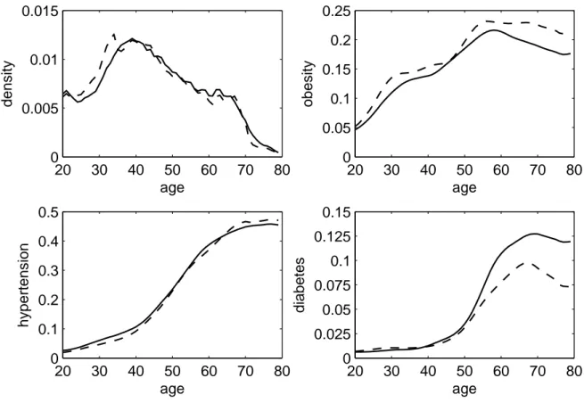
3.1 Kernel density and age-specific prevalences (pooled sample 2002, 2006) . . . 39

3.2 Age-specific income and Gini indices (pooled sample 2002, 2006) . . . . 41

3.3 Age-specific inequality of obesity (pooled sample 2002, 2006) . . . . 42

3.4 Age-specific inequality of hypertension (pooled sample 2002, 2006) . . . . . 43

3.5 Age-specific inequality of diabetes (pooled sample 2002, 2006) . . . . 44

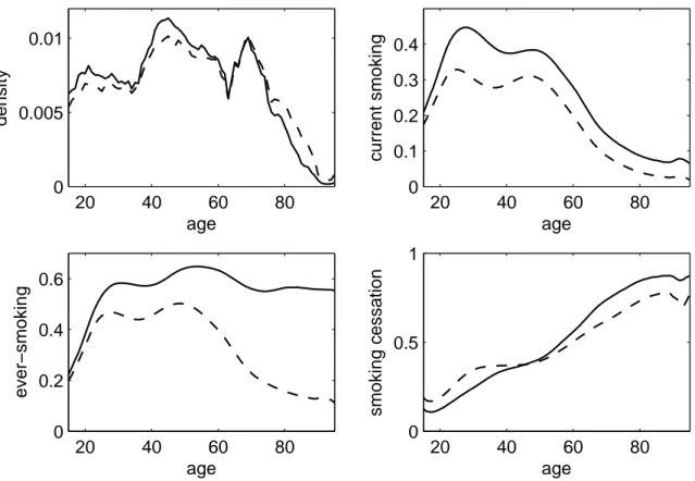
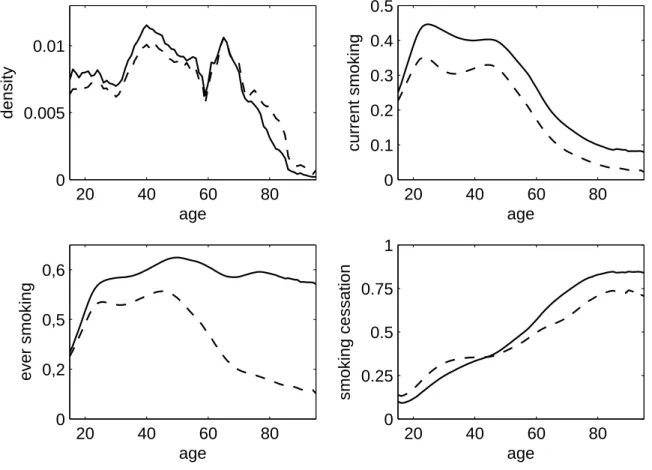
4.1 Descriptive figures (2009 sample) . . . . 56

4.2 Age-specific inequality of current smoking (2009 sample) . . . . 58

4.3 Age-specific inequality of ever-smoking (2009 sample) . . . . 59

4.4 Age-specific inequality of smoking cessation (2009 sample) . . . . 61

4.5 Descriptive figures (2005 sample) . . . . 63

4.6 Age-specific inequality of current smoking (2005 sample) . . . . 64

4.7 Age-specific inequality of ever-smoking (2005 sample) . . . . 65

4.8 Age-specific inequality of smoking cessation (2005 sample) . . . . 66

4.9 Nonresponse to smoking module (2009 sample) . . . . 68

4.10 Nonresponse to smoking module (2005 sample) . . . . 69

5.1 Age-specific and standardized prevalences (pooled sample 2002, 2006) . . . . 84

5.2 Age-specific inequality of obesity, index from theory (pooled sample 2002, 2006) . . . . 91

5.3 Age-specific inequality of obesity, deprivation index from factor analysis (pooled sample 2002, 2006) . . . . 92

5.4 Age-specific inequality of hypertension, deprivation index from theory (pooled

sample 2002, 2006) . . . . 93

(6)

5.5 Age-specific inequality of hypertension, deprivation index from factor analy- sis (pooled sample 2002, 2006) . . . . 94 5.6 Age-specific inequality of diabetes, deprivation index from theory (pooled

sample 2002, 2006) . . . . 96 5.7 Age-specific inequality of diabetes, deprivation index from factor analysis

(pooled sample 2002, 2006) . . . . 97 5.8 Deprivation-specific descriptive figure, deprivation index from theory (pooled

sample 2002, 2006) . . . . 98 5.9 Deprivation-specific descriptive figure, deprivation index from factor analysis

(pooled sample 2002, 2006) . . . . 99 5.10 Deprivation-specific income and Gini indices, deprivation index from theory

(pooled sample 2002, 2006) . . . 101 5.11 Deprivation-specific income and Gini indices, deprivation index from factor

analysis (pooled sample 2002, 2006) . . . 102 5.12 Deprivation-specific inequality of obesity, deprivation index from theory (pooled

sample 2002, 2006) . . . 103 5.13 Deprivation-specific inequality of obesity, deprivation index from factor anal-

ysis (pooled sample 2002, 2006) . . . 104 5.14 Deprivation-specific inequality of hypertension, deprivation index from theory

(pooled sample 2002, 2006) . . . 105 5.15 Deprivation-specific inequality of hypertension, deprivation index from factor

analysis (pooled sample 2002, 2006) . . . 106 5.16 Deprivation-specific inequality of diabetes, deprivation index from theory (pooled

sample 2002, 2006) . . . 107 5.17 Deprivation-specific inequality of diabetes, deprivation index from factor anal-

ysis (pooled sample 2002, 2006) . . . 108

(7)

List of Tables

3.1 Descriptive statistics (pooled sample 2002, 2006) . . . . 40

4.1 Descriptive smoking statistics (2009 sample) . . . . 55

4.2 Descriptive smoking statistics (2005 sample) . . . . 62

5.1 Domains of the German Index of Multiple Deprivation . . . . 77

5.2 Correlation matrix of overall deprivation ranks (pooled sample 2002, 2006) . 86 5.3 Rank sensitivity: household income and Index of Multiple Deprivation de- rived from the literature (pooled sample 2002, 2006) . . . . 88

5.4 Rank sensitivity, Indices of Multiple Deprivation with theory and factor anal-

ysis based weighting (pooled sample 2002, 2006) . . . . 90

(8)

(9)

Chapter 1 Introduction

“In any discussion of social equity and justice, illness and health must figure as a major concern. [...] First, health is among the most important conditions of human life and a critically significant constituent of human capabilities which we have reason to value. Any conception of social justice that accepts the need for a fair distribution as well as efficient formation of human capabilities cannot ignore the role of health in human life and the opportunities that persons, respectively, have to achieve good health - free from escapable illness, avoidable afflictions

and premature mortality.” Amartya Sen

¹

The relevance of equity in health for a fair and equitable development of human resources and societies, respectively, has been well explained by Sen (2002). Individual incomes, social arrangements, genetic propensities, working conditions and the epidemiological environments are among the factors which may contribute to health achievements or failures. In his article, Sen (2002) points out that discussions on equity in health should by no means be restricted to the question how health care is distributed. Although Sen stresses that health inequity is not equivalent to health inequality and that concentrating on the latter is not sufficient to assess

1Amartya Sen: Why Health Equity? Keynote Address to the Third Conference of the International Health Economics Association; York, 23 July 2001 (published in Health Economics as Sen, 2002)

(10)

the former, he still agrees that inequalities in health are a matter of interest of its own. “It (health inequality) does have interest of its own, and it certainly is a very important part of our understanding of health equity, which is a broader notion” (Sen, 2002, p. 662). Needless to say that equity should be considered as a concept which is probably neither objective nor directly measurable, but rather a social and political consensus to be found. The present thesis tries to contribute to this process by extending the empirical basis. More precisely, it is focused on the introduction and application of a new econometric approach to measure variations in health inequalities.

The concentration index is an adaptive tool for the measurement of income-related inequal- ities which offers some advantages over techniques such as, say, comparisons of prevalences in income quintiles or other population subgroups. In order to explain the causes of health sector inequalities, Wagstaff et al. (2003) propose the decomposition of the concentration in- dex to measure the contribution of demographic and socioeconomic characteristics to total health inequality. Using the marginal effects of these variables on the health outcome, they compute the respective elasticities and rewrite the concentration index of the health variable as the sum of the concentration indices of the explanatory variables weighted by their respective elasticities. From this decomposition approach, one may infer how health inequality would change if, say, no demographic effects were present.

²

Jones and López Nicolás (2006) further separate the contribution of response heterogeneity from the unexplained (residual) part in the decomposition formula derived by Wagstaff et al. (2003). They point out that response het- erogeneity in the elasticities may change the composition of health gradients considerably.

³

During a research project on health and health care utilization inequalities in Germany (Lün- gen et al., 2009), however, a major shortcoming of both decomposition approaches became evident: They do not allow comparisons of inequalities across age groups. When trying to gain a better understanding of the origins of health inequalities in Germany, the question in

2Note that this method has extensively been applied in Lüngen et al. (2009).

3More precisely, Jones and López Nicolás (2006) analyze heterogeneity in terms of age and sex.

(11)

which age groups inequalities could actually be observed came up repeatedly. At the time the research described in Lüngen et al. (2009) was finished, there seemed to be no suitable method to measure age-specific income-related health inequalities.

This lack of suitable methods to describe variations in health inequalities is the point of departure for the present thesis. Chapter 2 presents a new econometric approach to measure variations in inequalities with respect to some other continuous or discrete explanatory vari- able. The proposed model combines the well-established concentration index with the smooth coefficient model introduced by Li et al. (2002) to a semiparametric inequality index. The chapter introduces the model and presents a feasible estimator which is applied to data on self- assessed health from the 2005 and 2009 surveys of the German microcensus. It is found that the extent of health inequalities varies considerably between age groups. While no inequal- ities to the detriment of the poor are observed among children and the elderly, considerable health disadvantages are found among the economically deprived particularly in later mid-life.

The method is compared with the results obtained when estimating concentration indices for five year interval age groups. The estimator’s behavior in smaller samples is assessed through drawing subsamples from the data. The results suggest that the index works well for normal and large sized samples with more than thirty to forty thousand observations.

One may argue that the health variable in chapter 2 is rather general and subjective. Chapter 3 uses data on specific diseases drawn from the TNS Health Care Access Panel. Using the methods introduced in chapter 2, age-specific variations of income inequalities and income- related health inequalities in obesity, hypertension and diabetes are addressed. The results show that the social gradients concerning the prevalence of the diseases under consideration vary considerably with age in the female sample. Interestingly, only marginal variations are found in the male sample. Similar to chapter 2, the strongest inequalities to the detriment of the economically deprived are found in later mid-life.

While chapters 2 and 3 illustrate health outcomes, chapter 4 addresses smoking as an addic-

(12)

tive behavior being a major threat to one’s health. Sen (2002) stresses the distinction between a free decision not to care for one’s health and failure to achieve good health because of inade- quate social arrangements and lacking resources. He points out that “indeed even smoking and other addictive behaviour can also be seen in terms of a generated ‘unfreedom’ to conquer the habit” Sen (2002, p. 660). The method from chapter 2 is applied to data from the 2005 and 2009 surveys of the German microcensus. Chapter 4 addresses the prevalence of current and ever-smoking as well as smoking cessation. The result suggest that men are, on average, more likely to be current smokers and ever-smokers than women. Current and ever-smoking are both concentrated in worse-off households in younger birth cohorts. Smoking cessation is concentrated among the better-off in all age groups. The results from the 2005 and 2009 samples are quite similar. This may be seen as a hint that the microcensus data on smoking are fairly reliable.

⁴

Although age-specific variations in health inequalities have been in the main focus in chap- ters 2, 3 and 4, the varying inequality index is by no means restricted to age. The factor by which inequalities are allowed to vary may be replaced by any meaningful variable. As an ex- ample, the Index of Multiple Deprivation used by Maier et al. (2011) is employed in chapter 5 as both, the socioeconomic status variable and in place of age. The present thesis goes beyond a pure application of the German Index of Multiple Deprivation and uses the within-domain rankings to propose an empirically driven weighting scheme based on factor analysis. Com- paring the theory driven and the empirically driven approaches, it is found that the weighting scheme derived from factor analysis puts considerably more emphasis on income and unem- ployment rates than the index derived from the literature. Both deprivation indices are highly correlated and produce similar rankings, though. As in chapter 3, data on obesity, hyperten- sion, diabetes, income, age and sex are drawn from the TNS Health Care Access Panel. The

4Note that no household should have participated in both surveys as they are only included in four subsequent waves and are removed then. Hence, the last households included in 2005 were removed in 2008 and the samples are non-overlapping. The comment that the microcensus data are fairly reliable is motivated by the fact that the two non-overlapping samples produce almost equivalent results.

(13)

results for age-specific community deprivation-related health inequalities are similar to those found for age-specific income-related inequalities. The results for the deprivation-specific variations of income-related health inequalities, however, yield no significant variations. It is found in chapter 5 that the results obtained when using the theory driven and the empirically driven deprivation indices look rather similar. When measured for communes with similar deprivation status, income-related health inequalities are less marked than the overall-sample income-related inequalities. They do, however, not vary with the community deprivation rank.

In summary, this thesis presents evidence that income-related inequalities to the detriment of the economically deprived households exist in Germany. While this holds for health status in almost all age groups, smoking only concentrates among the worse-off households in younger cohorts. Considering the results for ever-smoking as a cohort effect, the results suggest that smoking indeed changed from a pro-rich towards a pro-poor habit over the twentieth century.

While individual income and community deprivation are similarly associated to individual

health, income-related health inequalities do not vary with community deprivation.

(14)

(15)

Chapter 2 Semiparametric modeling of age-specific variations in income-related health

inequalities ¹

2.1 Introduction

The existence of socioeconomic gradients in the distribution of health to the detriment of the deprived is firmly established among health economists (Balia and Jones, 2008; Erreygers, 2009; Humphries and van Doorslaer, 2000; van Doorslaer et al., 1997; van Doorslaer and Koolman, 2004; van Doorslaer et al., 2004; Jones and López Nicolás, 2006; Wagstaff et al., 1991; Wagstaff and van Doorslaer, 2000; Wagstaff et al., 2003). Little is known, however, about the mechanisms through which different socioeconomic factors affect health status and its distribution over the life course (van Kippersluis et al., 2009, 2010). Adding the life course perspective supports, for instance, the notion that labor force participation contributes sub- stantially to the socioeconomic gradient in health in the U.S. (Case and Deaton, 2005), Great

1This chapter is based on a manuscript co-authored by Karl Mosler.

(16)

Britain (Banks et al., 2007) and the Netherlands (van Kippersluis et al., 2010).

The literature has long been divided into two competing hypotheses explaining why dispar- ities in health may differ over the life course: the disadvantage accumulation hypothesis and the age as leveler hypothesis (Dupre, 2007). Both hypotheses agree that low socioeconomic status and lacking resources are associated with less healthy lifestyles, higher health risks, a faster decline of health status and higher mortality rates. The disadvantage accumulation hypothesis argues that social gradients in health develop in early life and become stronger as socioeconomic and health disadvantages accumulate over the entire life course (Kim and Durden, 2007; van Kippersluis et al., 2010; Lynch, 2003; Mirowsky and Ross, 2005; Prus, 2004; Ross and Wu, 1996; Willson et al., 2007). The age as leveler hypothesis adds the as- sumption that the decline of health is an unavoidable part of aging. Followers of the age as leveler hypothesis argue that health inequalities evolving from socioeconomic disadvantages increase up to some point in midlife but are then outperformed by the decline in health status due to aging and to some extent attenuated by a relief through retirement (Case and Deaton, 2005; Deaton and Paxson, 1998; Elo and Preston, 1996; Kim and Miech, 2009; van Kipper- sluis et al., 2010; Kunst and Mackenbach, 1994). The two hypotheses have long been treated as competing. However, van Kippersluis et al. (2010) argue that evidence found for the age as leveler hypothesis is also consistent with the disadvantage accumulation hypothesis. Some au- thors stress that leveling may be an artificial result due to mortality selection, though Beckett (2000) points out that this needs not necessarily be true for self-reported health.

A common approach to measure health inequalities is the concentration index. Although

it requires some ranking, say, by income, its computation does not require predefined socio-

economic groups. Using data from eleven European countries, van Kippersluis et al. (2009)

define age cohorts and compute batteries of concentration indices for each country. Since the

bounds of the concentration index depend on minimum, maximum and mean of the respec-

tive variable, they correct their indices following Erreygers (2009) to assure comparability

(17)

2.2 Methods

between age groups and countries. Their graphical comparisons support the accumulation hypothesis for most countries, however, their results favor the age as leveler hypothesis for France, Germany and the U.K.

This chapter introduces a varying inequality index for dichotomous health variables which does not require a priori sample stratification. As in van Kippersluis et al. (2009), the objective of this chapter is to describe the differences in income-related health inequalities across age cohorts. One may consider estimating a nonparametric smoother through age-specific con- centration indices as an alternative, however, this approach would reduce the reliability of the results considerably. The number of observations in predefined age groups of, say, five year intervals may be rather small resulting in high uncertainty particularly among the oldest age groups. Further, the estimates for ages close to the upper (lower) cohort limits would only be subject to the younger (older) individuals within the same cohort and hence likely be biased.

Smoothing over such results in a second step would then add its own uncertainty and lead to fairly imprecise results. Based on the varying coefficient model (Hastie and Tibshirani, 1993;

Li et al., 2002), a semiparametric extension of the convenient regression approach (Kakwani et al., 1997) is proposed here. Using kernel smoothing techniques and a locally chosen band- width allows to estimate the functional relationship between the concentration index and age.

The varying index is adjusted using Wagstaff’s (2005) correction formula for binary variables with local estimates of the mean.

2.2 Methods

2.2.1 The concentration index

In their paper, Wagstaff et al. (1991) introduce the concept of concentration curves and in-

dices to the field of health inequality analyses. The concentration index C stems from the

concentration curve where the cumulative share of some health variable y is plotted against

(18)

the cumulative share of the population ranked by socioeconomic position (Wagstaff et al., 1991). It measures twice the area between the concentration curve and the line of equality.

C is bound in the ( − 1; 1) interval and becomes positive (negative), if the variable of interest concentrates among the rich (poor). C is zero if no income-related inequality is observed.

Using the covariance approach in Lerman and Yitzhaki (1989), Kakwani et al. (1997) present the regression formula for the concentration index

2 σ

²_r

µ y = β

0

+ β

1

r + ε, (2.1)

where µ is the mean of the health variable and r is the fractional rank with variance σ

²_r

. Equa- tion (2.1) can be estimated using linear regression models to obtain the concentration index as C = β

1

.

2.2.2 Varying coefficient models

In the framework of varying coefficient models, Li et al. (2002) propose a semiparametric smooth coefficient model based on locally weighted least squares regression. With X denot- ing the regressor matrix and y the dependent variable, the elements of the coefficient vector (β

0

, ..., β

Q

) are modeled as smooth functions of another regressor z which varies in some Z ⊂ R :

y = β

0

(z) +

∑

Q q=1

β

q

(z)x

q

+ ε. (2.2)

This model can be estimated using nonparametric smoothing techniques (see Li et al., 2002;

Hastie and Tibshirani, 1993) from

β(z) = E(X

^′

X | z)

₋1

E (X

^′

y | z), (2.3)

(19)

2.2 Methods

where X = (1 x

1

. . . x

_Q

). Li et al. (2002) have shown that, for increasing numbers of observa- tions n, the estimator ˆ β(z) obtained from (2.3) asymptotically follows a normal distribution, i.e. √

nh

z

β(z) ˆ − β(z)

∼ N(0, Ω(z)); see section 2.2.5 for the estimation of the covariance matrix.

2.2.3 A semiparametric inequality index

Combining the weighted regression approach from equation (2.1) with the varying coefficient model (2.2), the proposal for a semiparametric convenient regression formula is

2 σ

²_r

(z)

µ(z) y = β

0

(z) + β

1

(z) r(z) + ε, (2.4) such that C(z) = β

1

(z), z ∈ Z. Note that the concentration index is a bivariate extension of the Gini index; if y is the social status variable, equation (2.4) works as a semiparametric Gini index. The local mean µ(z) can be estimated nonparametrically. The weighted fractional rank r(z) has to be written as a function of z. Intuitively, when estimating a varying concentration index, one will be interested in the observable inequality given z. Hence, taking into account all subjects in the sample for computing r regardless of their individual values of z would be misleading. Technically, the condition that the sum of the sample weights has to equal 1 and the mean and variance of the weighted fractional rank have to be 0.5 and

¹

/

¹²

, respectively, must hold (Lerman and Yitzhaki, 1989). This can only be fulfilled if the weighted fractional rank is computed using only those individuals included in the local regression and incorporat- ing the kernel weights k

hz

(u

i

):

r

_i

(z) =

∑

i j=1

w

_j

(z)k

hz

(u

j

) − w

_i

(z)k

hz

(u

i

)

2 . (2.5)

The vector of sample weights w(z) must be rescaled such that ∑

ⁿ_i=1

w

i

(z) k

_h_z

(u

i

) = 1 for each

z ∈ Z. Note that the mean and variance of r(z) are then (asymptotically) sample independent

(20)

and do not vary with z.

For binary variables, the bounds of the concentration index depend inversely on the vari- able’s mean, | C | ≤ 1 − µ (see Wagstaff, 2005, 2011; Erreygers, 2009). For an intuitive explana- tion, first assume a constant equal to 1. With no difference between individuals, concentration among rich or poor is impossible; the concentration index equals zero. Now consider, say, 10 percent ones and 90 percent zeros. Ordering the variable by itself, one would obtain a Gini in- dex of 0.9; the largest possible concentration. Analogously, the maximum possible inequality for a binary variable with 90 percent ones and 10 percent zeros would equal 0.1 (see Wagstaff, 2011, for a graphical illustration). Comparisons of concentration indices of binary variables with rather different means may thus be misleading.

There is an ongoing discussion on possible correction methods for concentration indices of limited variables (Erreygers, 2009; Wagstaff, 2005, 2011) with a dissent between the authors on how a corrected index should react to changes of the mean. Considering the above example, Erreygers (2009) would argue that an increase from 10 to 20 percent implies a decrease in inequality as now the second richest (poorest) decile is also affected. The argument in Wagstaff (2005, 2011) is that, as still only the richest (poorest) are affected, the new situation still corresponds with the maximum possible inequality. A reaction of the index to pure prevalence changes would not be desirable here as the motivation of this chapter is to compare inequalities across age groups and sexes. The proposal is to adapt the formula in Wagstaff (2005, 2011) as a pointwise correction of the semiparametric concentration index using the local mean µ(z) of y:

W (z) = C(z)

1 − µ(z) . (2.6)

(21)

2.2 Methods

2.2.4 Estimation

Applying a consistent Nadaraya-Watson estimator, sample weights are taken into account and C(z) = ˆ β ˆ

1

(z), z ∈ Z, is obtained by computing

β(z) = ˆ

"

∑

n i=1

k

_h_z

(u

i

)w

i

(z) X

_i^′

X

_i

#

₋1

"

∑

n i=1

k

_h_z

(u

i

)w

i

(z) X

_i^′

y ˜

_i

#

. (2.7)

Note that ˜ y

_i

=

²^σ²^r^(z)

/

^µ(z)

y

_i

and X

_i

= (1 r

_i

(z)) depend on z as the local mean and the local fractional rank from equation (2.5) are involved (for simplicity, X

_i

is written in place of X

_i

(z) here). The kernel weights are k

_h_z

(u

i

) = K

_h_z

(u

i

) h

∑

ⁿ_j=1

K

_h_z

u

j

i

₋1

with u

i

= z

i

− z. The quartic kernel K(u

i

) = (

¹⁵

/

16

) 1 − u

²_i

2

I

|u_i|<1

with K

₂²

= ´

_∞

−∞

K

²

(u) du =

⁵

/

7

is used, where I

^A

is an indicator function of restriction A. The bandwidth h

_z

is included such that K

_h_z

( · ) = (h

z

)

⁻¹

K (

^·

/

^hz

). The quartic kernel assigns higher weights to observations closer to z (smaller u

_i

), lower weights for observations further away from z (larger u

_i

) and zero weights if an observation is outside the bandwidth.

²

Although the estimator is asymptotically unbiased (Li et al., 2002), any nonparametric regression in finite samples suffers to some extent from a tradeoff between bias and variability: decreasing the bandwidth parameter decreases the bias but at the cost of increasing uncertainty; and vice versa (see also Bilger, 2008, for a discussion). This problem is addressed here by choosing the bandwidth inversely to the local data density as h

_z

= 1.06 ˆ σ

z

n

⁻^0.2

f ˆ

_z⁻^0.3

, where ˆ f

_z

is the estimated kernel density at a particular value of z and ˆ σ

z

is the standard deviation of z obtained from the sample. Fan and Gijbels (1992) have shown that adaptive local smoothers generally yield good results and, in addition, avoid the well-known boundary effect.

To obtain confidence intervals for the semiparametric concentration index, its standard er- ror needs to be estimated. Kakwani et al. (1997), Wildman (2003) and O’Donnell et al.

(2008) argue that it is not sufficient to estimate the standard error of β

1

(z) from equation

2For K_h_z(ui), restriction A is|u_i|<h_zmaking the indicator function 1 if|u_i|<h_zand 0 otherwise.

(22)

(2.1) because of the sample variability of µ(z). One may estimate β

₀

(z) and β

₁

(z) from y = β

^∗₀

(z) + β

^∗₁

(z)r(z) + ε

^∗

and consider the concentration index as a nonlinear combination of the two coefficients with β

^∗₀

(z) + 0.5β

^∗₁

(z) in place of µ(z). The variance can be approx- imated using the δ method (Rao, 1965) on C(z) ≈ 2σ

²_r

(z)

β

^∗₀

(z) + 0.5β

^∗₁

(z)

₋1

β

^∗₁

(z) for the semiparametric concentration index.

³

The variance of the varying Wagstaff index W (z) can be estimated analogously.

⁴

Further, it has been argued that the covariance matrix from a sim- ple OLS regression is not wholly accurate because the error term ε

^∗

may be autocorrelated and heteroscedastic (Kakwani et al., 1997). This chapter follows Wildman (2003) who proposes using the order of the rank variable in place of time to compute pointwise heteroscedasticity and autocorrelation consistent Newey-West covariance matrices (see section 2.2.5 for details).

2.2.5 Variance estimation

According to Li et al. (2002), the covariance matrix Ω(z) in the semiparametric varying coef- ficient model is

Ω(z) =

f

z

E X

^′

X | z

₋1

Φ(z)

f

z

E X

^′

X | z

₋1

(2.8)

3This yields

σ²_C(z)≈4σ⁴_r(z)β²₀(z)σ11(z) +β²₁(z)σ22(z)−2β1(z)β0(z)σ12(z) (β0(z) +0.5β1(z))⁴

for the varianceσ²_C(z)of C(z), where theσi j(z)are the i jth elements of the covariance matrixΩ(z)ofβ(z).

4Equation (2.6) for W(z)can be written as

W(z) = C(z)

1−µ(z)≡ 2σ²_r(z)

(β0(z) +0.5β1(z))(1−β0(z)−0.5β1(z))β1(z).

One may then estimate the varianceσ²_W(z)of W(z)as

σ_W²(z) ≈ 1

36 β0(z) +¹₂β1(z)4

1−β0(z)−¹₂β1(z)4

×

β²₀(z)σ22(z)

(1−β0(z))²−1

2β0(z)β²₁(z)

+β²₁(z)σ11(z) 1−4(1−β1(z))β0(z)−2β1(z) +4β²₀(z) +β²₁(z)

+σ12(z)β0(z)β1(z) −2+6β0(z)−4β²₀(z) +β²₁(z) +2β1(z)−2β0(z)β1(z) +1

16β³₁(z) (8β1(z)σ12(z) +β1(z)σ22(z)−8σ12(z)) +1

2σ22(z)β0(z)β²₁(z)

.

(23)

2.3 Data and variables with Φ(z) = f

_z

E X

^′

X σ

²_ε

(z) | X, z K

₂²

and σ

²_ε

(z) = E (ε

²_i

| X , z). To estimate a heteroscedas- ticity and autocorrelation consistent covariance matrix ˆ Ω

hac

(z), Φ(z) must be adapted accord- ingly. Following the proposal by White (1980), Φ(z) is computed as

Φ ˆ

hac

(z) = f

_z

Ψ

0

(z) +

∑

m j=1

ω

j,m

Ψ

j

(z)

! K

₂²

. (2.9)

with

Ψ

j

(z) =

∑

n i=j+1

k

_h_z

(u

i

)w

i

(z) ε

i

ε

i−j

x

i

x

^′_i₋_j

+ x

i−j

x

^′_i

(2.10) and Ψ

0

= ∑

ⁿ_i=1

k

_h_z

(u

i

)w

i

(z)ε

²_i

x

^′_i

x

_i

. Bartlett weights ω

j,m

= 1 −

^j

/

^(m+1)

are applied to assure a positive semi-definite covariance matrix (Newey and West, 1987), E (X

^′

X | z) and the kernel density are computed as above.

2.3 Data and variables

Data for the empirical application were drawn from the 2005 survey of the German microcen- sus provided by the Research Data Centers of the Federal Statistical Office and the Statistical Offices of the Federal States (Forschungsdatenzentren der Statistischen Ämter des Bundes und der Länder). The microcensus is Europe’s largest annual country-wide survey with one percent of the German households (approximately 820, 000 individuals) being interviewed.

Households are included in four consecutive surveys and 25 percent of the households are

replaced each year. In 2005, the vast majority of interviews was conducted by trained staff as

face to face interviews. Answers were recorded directly into the data collection software. The

rate of self-fillers was approximately twelve percent. The microcensus comprises an annu-

ally surveyed socioeconomic module for which response is mandatory. A health related part

for which responding was voluntary was included in 2005. Due to sample size and manda-

tory response, the German microcensus can be seen as one of the most representative samples

(24)

available (see FSO, 2006 or Reeske et al., 2009).

The scientific use file (SUF) available for non-profit research organizations is used for the empirical illustration. The SUF comprises a randomly drawn subsample of approximately 70 percent (n = 477, 239) of the German microcensus. Inverse probability weights accounting for the regional, age and sex specific composition of the sample are provided by the Federal Sta- tistical Office (see Lechert and Schimpl-Neimanns, 2007, for a technical report). Removing 92, 458 individuals from the sample owing to missing information leaves n = 384, 781 obser- vations (198, 877 female and 185, 904 male) for the empirical analysis. The inverse probability weights were adjusted accordingly.

The health outcome variable is a subjective measure of health, i.e. whether an individual experienced illness including chronic diseases during the preceding four weeks. Although positive responses may include (common) acute diseases such as colds or light flues, one may assume that these affect all socioeconomic groups. The health outcome is measured via the question “have you been ill (including chronic diseases) or injured by an accident during the last four weeks” with possible answers “yes, ill”, “yes, injured”, “no” or “no statement”. The analysis is restricted to having been ill and a binary variable with outcome 1 for “yes, ill” is generated. The options “no” and “yes, injured” were both treated as “not ill” and hence coded as 0. Assuming that only those who actually felt affected would consider themselves as ill, this measure of health has the advantage that it only includes diseases if they were relevant to the respective individual.

Household income is used to assess an individual’s relative socioeconomic position (note

that this is not restricted to a particular source of income in the data). One may consider this

as unsuitable for some countries particularly after retirement. However, Germany is an ex-

emption because its welfare policies can be seen as rather status preserving (Brockmann et al.,

2009). Approximately 90 percent of the German population are covered by the public pension

system where benefits after retirement depend on compulsory contributions subtracted from

(25)

2.4 Results

0 20 40 60 80

0 0.001 0.002 0.003 0.004

age

density

0 20 40 60 80

0 0.05 0.1 0.15 0.2 0.25

age

prevalence

Figure 2.1: Descriptive figures (2005 sample)

Empirical density of age (left) and smoothed age-specific prevalence of sickness within the preceding four weeks (right) for males (solid lines) and females (dashed lines).

the gross income (for a description of the German public pension system, see Boersch-Supan and Wilke, 2004). Therefore, considerable changes of the relative socioeconomic position within one’s age group after retirement seem unlikely and household income can be seen as a suitable indicator for the socioeconomic position over the entire life course. The modified OECD equivalence scale is used to compute net equivalent household income. Equivalence weights are assigned as follows: 1 for the first adult, 0.5 for each additional person aged 14 or older and 0.3 for children younger than 14 (see e.g. van Doorslaer et al., 2004; van Kippersluis et al., 2009).

2.4 Results

2.4.1 Results from the 2005 sample

The left graph in figure 2.1 describes the kernel density estimate ˆ f

_z

of the nonparametric

smoothing regressor z (age). The graphs for the male and female samples imply that the largest

bandwidth parameter was used for subjects older than 80 for both sexes. The distribution of

(26)

age groups corresponds with the population pyramid for Germany. Without adjusting for mortality, birth cohorts younger than 40 (i.e. born after 1965) are smaller than those born earlier. One may see this as evidence for an aging society (see e.g. von Weizsäcker, 1996).

The right graph in figure 2.1 presents the smoothed age-specific prevalence of illness within the preceding four weeks. The graphs suggest that children younger than 10 have a higher prevalence than individuals aged between 10 and 40 years. From 45 years onward, prevalence increases almost linearly and stagnates for the elderly older than 80. While the prevalence is somewhat lower for female children, the graph suggests that it is slightly higher among female adolescents and adults until around 45 and for elder women over 80.

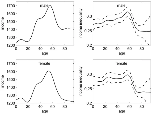
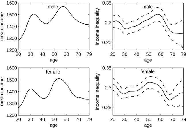
The upper and lower left graphs in figure 2.2 present the age-specific means of the net equivalent household incomes for males and females, respectively. Considering that income is assigned equally to each household member, the graphs suggest that households with chil- dren have, on average, the lowest net equivalent household income. While the age-specific mean income does not differ between sexes for children, adult men have, on average, higher incomes. The sex difference appears to be highest for the oldest (over 75). Between the age of 20 and 60, one may say that the older an individual the higher is the expected net equivalent household income. The bump around age 40 for in both graphs stems from the higher average number of dependent children which increases the equivalence weights in the corresponding households. The expected mean income peaks around 57, decreases with retirement (i.e. for subjects aged between 57 and 70) and varies around 1, 400 Euro for males and 1, 200 Euro for females older than 70.

The homogeneous (age-independent) Gini index is 0.282 with a standard error of 0.0033

for the female and 0.2915 with a standard error of 0.0036 for the male sample. The right hand

graphs in figure 2.2 present the corresponding age-specific Gini indices. The age-specific

index varies around 0.27 for children and adolescents in both samples. For males over 20, the

graph suggests an increasing income inequality which peaks at age 57 with a Gini of 0.32. In

(27)

2.4 Results

0 20 40 60 80

1200 1300 1400 1500 1600 1700

age

income

male

0 20 40 60 80

1200 1300 1400 1500 1600 1700

age

income

female

0 20 40 60 80

0.2 0.25 0.3

age

income inequality

male

0 20 40 60 80

0.2 0.25 0.3

age

income inequality

female

Figure 2.2: Age-specific income and Gini indices (2005 sample)

Age-specific mean (left) and Gini indices (right) with 95 percent confidence intervals (dashed lines) of net equivalent household income for males (top) and females (bottom).

the female sample, income inequality is somewhat higher among adults (Gini of 0.28) than among children. It increases between 50 and 60 and peaks at age 58 with a Gini of 0.3. With the retirement age, the index drops back to approximately 0.25 for both sexes.

Computing the homogeneous concentration indices for the four weeks prevalence of illness

yields − 0.0606 with a standard error of 0.0026 for the female and − 0.0653 with a standard

error of 0.0028 for the male sample. The homogeneous Wagstaff indices are − 0.0696 with a

standard error of 0.0074 for the female and − 0.0738 with a standard error of 0.0079 for the

male sample. The negative and highly significant concentration and Wagstaff indices suggest

(28)

0 10 20 30 40 50 60 70 80 90

−0.2

−0.1 0 0.1

age

inequality

male

0 10 20 30 40 50 60 70 80 90

−0.2

−0.1 0 0.1

age

inequality

female

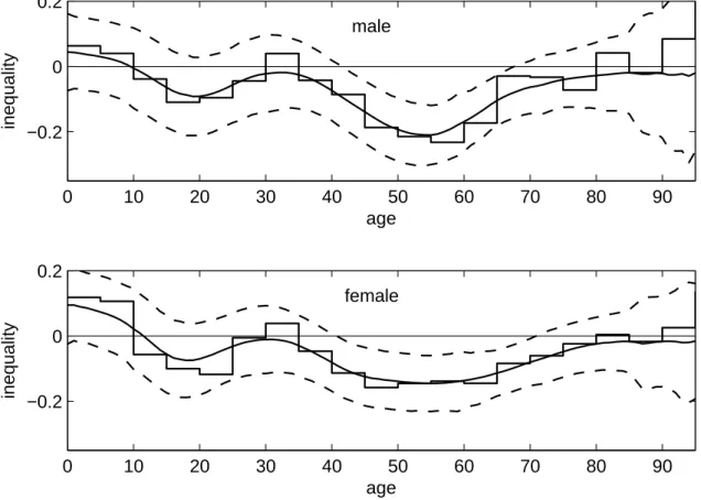
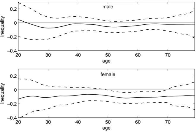
Figure 2.3: Varying inequality index (2005 sample)

Age-specific inequality indices (solid lines) with 95 percent confidence intervals (dashed lines) for males (top) and females (bottom); the step function represents concentration indices com- puted for five year age groups.

a considerable concentration of illness among the poor.

The varying Wagstaff indices in figure 2.3 vary around the homogeneous estimates. The

graph for the male sample suggests a statistically insignificant concentration of illness among

the better-off for children younger than 14. Illness is significantly concentrated among males

in lower income households in the age groups between 19 and 26 as well as between 33 and

77. There is no significant concentration among elder males over 77. The graph for the female

sample suggests a significant concentration of illness among higher income households for

children younger than 5. As in the male sample, the index for females shifts from a concen-

(29)

2.4 Results

tration among the better-off towards a concentration among the worse-off in late childhood.

Significant concentration among females in lower income households is found for those be- tween 17 and 25 as well as between 39 and 74. No significant concentration is found for the elderly over 74. Considerable sex-specific differences in the curve shapes are only found for the 20 to 40 years old. While there is some flattening for the male sample, inequality is lower among females in this age group than around the 20 as well as the 40 to 70 years old.

Comparing the results of the varying and the homogeneous Wagstaff indices, it is observed that the homogeneous index significantly underestimates the concentration of illness among the lower income households for females between 44 and 65 and males between 44 and 67.

Conversely, the homogeneous indices would suggest a significant concentration of illness among children in lower income households while the age-specific indices yield opposite or insignificant results. The results from the index computed for five year age groups are some- what similar to those from the varying index where data are dense. However, the five year interval index exhibits several leaps and a considerably higher variability. Comparison of the two graphs demonstrates the above mentioned bias close to the group limits.

2.4.2 Results from the 2009 sample

⁵

The patterns of the kernel density estimates and the age-specific prevalences in figure 2.4 are similar to those in figure 2.1. It should be mentioned that the level of the kernel density estimate differs somewhat and that the estimated prevalence rates are higher across all age groups in the 2009 sample than in the 2005 sample for both sexes. The variations between age groups, however, are similar in both figures.

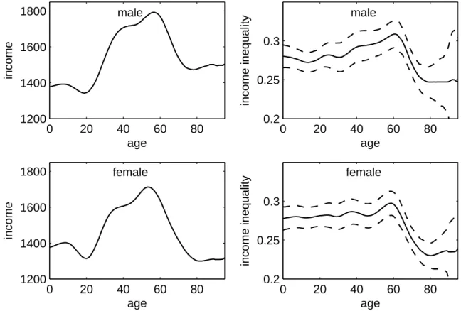
Comparing the results for income in figure 2.5 with those in figure 2.2, it is found that the age-specific mean net equivalent household income is higher in the 2009 sample than in the 2005 sample in all age groups and for both sexes. One may agree that this increase in incomes

5The 2009 microcensus is introduced in section 4.2.

(30)

0 20 40 60 80 0

0.005 age

density

0 20 40 60 80

0 0.1 0.2 0.3

age

prevalence

Figure 2.4: Descriptive figures (2009 sample)

Empirical density of age (left) and smoothed age-specific prevalence of sickness within the preceding four weeks (right) for males (solid lines) and females (dashed lines).

likely reflects inflation rates and increases in wages. The age-specific estimates of income inequalities in figure 2.5 do not differ noteworthy from those in figure 2.2. In summary, the results for income and income inequality are fairly similar in the 2005 and 2009 samples.

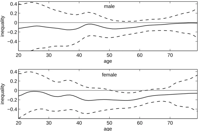
As in the figures concerning density, prevalence, income and income inequality, the observed age-specific income-related health inequality in figure 2.6 is fairly similar to that in figure 2.3.

One may agree that no considerable differences between both samples are evident here.

2.4.3 A note on smaller samples

As the varying inequality index introduced in this chapter has not been applied before, one may be interested in its smaller sample behavior. The following figures present estimates for the age-specific inequalities computed for random subsamples drawn from the underlying sample.

The results are compared with the concentration indices computed for five year intervals as suggested by van Kippersluis et al. (2009).

Figure 2.7 presents the estimates from a 50 percent subsample (92, 780 males and 99, 611

female). The results are similar to those in figure 2.3 and demonstrate that randomly halving

the sample does not change the results considerably. The results for the 25 percent (46, 493

(31)

2.4 Results

0 20 40 60 80

1200 1400 1600 1800

age

income

male

0 20 40 60 80

1200 1400 1600 1800

age

income

female

0 20 40 60 80

0.2 0.25 0.3

age

income inequality

male

0 20 40 60 80

0.2 0.25 0.3

age

income inequality

female

Figure 2.5: Age-specific income and Gini indices (2009 sample)

Age-specific mean (left) and Gini indices (right) with 95 percent confidence intervals (dashed lines) of net equivalent household income for males (top) and females (bottom).

males and 49, 702 females) subsample in figures 2.8 also do not differ considerably from the

full sample results in figure 2.3. When further reducing the sample size, the curves become

flatter and variations across age groups seem less pronounced. This can be observed in the

10 percent subsample (18, 523 males and 19, 955 females) in figure 2.9 and the 5 percent

subsample (9, 252 males and 9, 987 females) in figure 2.10. This flattening may to some extent

be caused by a selection bias despite the random sampling from the full sample, however, the

decreasing n may also have increased the degree of smoothing. It is further observed that the

confidence intervals widen with decreasing sample size n.

(32)

0 10 20 30 40 50 60 70 80 90

−0.2

−0.1 0 0.1

age

inequality

male

0 10 20 30 40 50 60 70 80 90

−0.2

−0.1 0 0.1

age

inequality

female

Figure 2.6: Varying inequality index (2009 sample)

Age-specific inequality (solid lines) with 95 percent confidence intervals (dashed lines) for males (top) and females (bottom).

2.4.4 A note on nonresponses

As responding to the health module was voluntary, one may be interested in the distribution of

nonresponses. Figures 2.11 and 2.12 demonstrate the age-specific income-related gradient of

nonresponses to the health module in the 2005 and the 2009 samples, respectively. It is found

that the patterns of inequalities in nonresponses are fairly similar in both samples. However,

the concentration of nonresponse among the worse-off is somewhat more pronounced and

considerably more significant in the 2009 sample. Under the assumption that the econom-

ically deprived are more affected by illness than the better-off, the observed concentration

of nonresponses among the worse-off may lead to some underestimation of the age-specific

income-related concentration of illness among them.

(33)

2.5 Discussion

0 10 20 30 40 50 60 70 80 90

−0.2

−0.1 0 0.1

age

inequality

male

0 10 20 30 40 50 60 70 80 90

−0.2

−0.1 0 0.1

age

inequality

female

Figure 2.7: 50 percent subsample (2005 sample)

Age-specific inequality indices (smooth solid line) with 95 percent confidence intervals (dashed line) and five year interval Wagstaff indices (step function); 50 percent subsample with 92, 780 males (top) and 99, 611 female (bottom) of the 2005 microcensus.

2.5 Discussion

In this chapter, the notion of concentration indices (Erreygers, 2009; Kakwani et al., 1997; van

Kippersluis et al., 2009; Wagstaff et al., 1991; Wagstaff, 2005) is combined with semipara-

metric regression techniques (Hastie and Tibshirani, 1993; Li et al., 2002) to a semiparametric

inequality index with some convenient properties. Using the varying bandwidth inverse to

local density, the index adapts itself to the data without a priori stratification into age or in-

come groups. This method allows an age-specific computation of the inequality index with

a sufficiently large number of observations guaranteed even where observations are scarce.

(34)

0 10 20 30 40 50 60 70 80 90

−0.2 0 0.2

age

inequality

male

0 10 20 30 40 50 60 70 80 90

−0.2 0 0.2

age

inequality

female

Figure 2.8: 25 percent subsample (2005 sample)

Age-specific inequality indices (smooth solid lines) with 95 percent confidence intervals (dashed lines) and five year interval Wagstaff indices (step functions); 25 percent subsample with 46, 493 males (top) and 49, 702 female (bottom) of the 2005 microcensus.

The quotient obtained through the local correction based on Wagstaff’s (2005) formula allows comparisons of the extent of inequality throughout the support of the smoothing regressor.

Considering the results for smaller subsamples, the overall impression is that the index per- forms well for samples larger than 40,000 to 50,000 observations. Where samples become considerably smaller (i.e. < 20, 000), however, it seems that the varying inequality index should be applied with caution.

Using German microcensus data, the power of the semiparametric approach to describe

age-specific income and income-related inequalities is demonstrated. Prus (2004) argues that

(35)

2.5 Discussion

0 10 20 30 40 50 60 70 80 90

−0.4

−0.2 0 0.2

age

inequality

male

0 10 20 30 40 50 60 70 80 90

−0.4

−0.2 0 0.2

age

inequality

female

Figure 2.9: 10 percent subsample (2005 sample)

Age-specific inequality indices (smooth solid lines) with 95 percent confidence intervals (dashed lines) five year interval Wagstaff indices (step functions); 10 percent subsample with 18, 523 males (top) and 9, 955 female (bottom) of the 2005 microcensus.

one would require panel data to test the accumulation hypothesis. Similar to e.g. van Kipper-

sluis et al. (2009), the aim of this chapter was to illustrate the variation of income and health

inequalities across age groups in Germany. As a main result, it is found that direction and

extent of the income-related inequality varies considerably with age. While children exhibit

pro rich inequality, strong inequalities to the detriment of the poor are observed for people

aged between 30 and 70. In line with van Kippersluis et al. (2009), the strongest inequality

is observed around the common age for retirement (note that the statutory age for retirement

in Germany is 65, however, most people retire between 58 and 64; see Wingerter, 2010). Ac-

(36)

0 10 20 30 40 50 60 70 80 90

−0.4

−0.2 0 0.2

age

inequality

male

0 10 20 30 40 50 60 70 80 90

−0.4

−0.2 0 0.2

age

inequality

female

Figure 2.10: 5 percent subsample (2005 sample)

Age-specific inequality indices (smooth solid lines) with 95 percent confidence intervals (dashed lines) and five year interval Wagstaff indices (step functions); 5 percent subsample with 9, 252 males (top) and 9, 987 females (bottom) of the 2005 microcensus.

cording to Dupre (2007), the leveling found among the retired may be an artificial effect owing to mortality selection as both decline of health and increase of mortality rates are faster among the worse-off. However, Beckett (2000) has shown that this needs not necessarily be true for self-reported health.

It seems unlikely that the observed leveling is solely an artificial effect evoked by mortality selection. Mortality rates in 2005 did not exceed 2 percent before the age of 68 (74) and 5 percent before the age of 77 (81) in the male (female) sample (see Human Mortality Database, 2012).

⁶

The results for those older than 80 should be treated with caution, though, as mortal-

6Mortality rates were similar in 2009.

(37)

2.5 Discussion

0 10 20 30 40 50 60 70 80 90

−0.2

−0.1 0 0.1

age

inequality

male

0 10 20 30 40 50 60 70 80 90

−0.2

−0.1 0 0.1

age

inequality

female

Figure 2.11: Nonresponse to health module (2005 sample)

Age-specific inequality indices (solid lines) with 95 percent confidence intervals (dashed lines) for nonresponse in the male (top) and female (bottom) samples to the voluntary health module included in the microcensus 2005.

ity may play a considerable role in these age groups. As the age-specific income inequality persists to some extent in older age, one may further consider it as unlikely that the decline in income-related health inequalities could simply be due to an equalization of the net equivalent household income after retirement.

⁷

7Note that technically, only income ranks, but not differences between incomes, matter. One may still consider it as possible that income equalizations may lead to a flattening of the income-related gradient if one considers income as relevant to health.

(38)

0 10 20 30 40 50 60 70 80 90

−0.2

−0.1 0 0.1

age

inequality

male

0 10 20 30 40 50 60 70 80 90

−0.2

−0.1 0 0.1

age

inequality

female

Figure 2.12: Nonresponse to health module (2009 sample)

Age-specific inequality indices (solid lines) with 95 percent confidence intervals (dashed lines) for nonresponse in the male (top) and female (bottom) samples to the voluntary health module included in the microcensus 2005.

2.6 Conclusions

One may conclude that the observed variations in age-specific health inequalities can be seen

as support the age as leveler hypothesis. The health gradient becomes pro-poor among adoles-

cents and is strongest in the late working life. As the reduction in health inequalities coincides

with a substantial increase in the age-specific prevalence, one may agree that a large part of

the observed leveling can be attributed to an age-related decline of health. No income-related

health inequality is observed in the female sample around age 30. As the average number

of dependent children is highest around this age, one may speculate that the flatter gradient

(39)

2.6 Conclusions

between 20 and 40 among females may be related to maternity.

(40)

(41)

Chapter 3 On age-specific variations in

income-related inequalities in diabetes, hypertension and obesity ¹

3.1 Introduction

With the introduction of the health concentration index (Wagstaff et al., 1991), socioeconomic gradients in the distribution of health became an important research field in health economics (see e.g. van Doorslaer et al., 2004, 2006; Kakwani et al., 1997; McKinnon et al., 2011).

Banks et al. (2007), Case and Deaton (2005) and van Kippersluis et al. (2010) point out that considering the life course perspective may be important for a better understanding of the origins of disparities in health.

The relation of low socioeconomic status and less healthy lifestyles, higher health risks and increased rates of premature mortality is well documented in the literature (Balia and Jones,

1A previous version of this chapter has been accepted for publication as Siegel M, Luengen M, Stock S. “On age-specific variations in income-related inequalities in diabetes, hypertension and obesity”. International Journal of Public Health, DOI: 10.1007/s00038-012-0368-7; downloadable from

http://www.springerlink.com/content/181l52078524547u/.

(42)

2008; Case and Deaton, 2005; Deaton and Paxson, 1998; Kim and Durden, 2007; Lynch, 2003; Prus, 2004). The two currently predominant explanations for variations in socioeco- nomic health gradients over the life course are the disadvantage accumulation hypothesis and the age as leveler hypothesis. The former states that social health gradients develop in early life and emerge over the complete life course through continual accumulation of health dis- advantages among the deprived (Kim and Durden, 2007; van Kippersluis et al., 2010; Lynch, 2003; Prus, 2004; Ross and Wu, 1996). The age as leveler hypothesis, on the other hand, has long been considered as an antithesis (Dupre, 2007). It is, however, rather an extension adding the assumption that the decline of health (being an inevitable part of aging) may outperform the accumulation of health disadvantages around mid-age (Case and Deaton, 2005; Deaton and Paxson, 1998; Kim and Miech, 2009; Kunst and Mackenbach, 1994). According to van Kippersluis et al. (2010), evidence for the age as leveler hypothesis is generally consistent with an accumulation process up to some point where age begins acting as a leveler in later life. Associating the accumulation process to the individual and leveling through age to the aggregate level, Dupre (2007) has shown that both mechanisms are by no means contradictory.

A growing body of literature analyzes the health status over the life course for distinct so- cioeconomic groups. van Kippersluis et al. (2010), for instance, use cross sectional data from the Netherlands and compare the development of self reported health, disability and mortal- ity for distinct educational groups. Mirowsky and Ross (2005) investigate differences in the predicted health status between educational levels in the United States. Both find that health status declines faster among the less educated. Using data from eleven European countries, van Kippersluis et al. (2009) find a continual disadvantage accumulation for most countries, however, they discover some leveling for France, Germany and the U.K.

No work has yet been done on the life course perspective in income-related inequalities of

specific diseases. The aim of this chapter is to highlight changes of the social gradients in

three health outcomes across different age groups. Using German survey data, age-specific

(43)

3.2 Data

variations in income-related health inequalities in hypertension and diabetes are investigated.

The risk of hypertension and diabetes is negatively correlated with socioeconomic status in de- veloped countries and both are considered as avoidable through lifestyle and health behavior (Harati et al., 2010; Puska, 2010). The present chapter further analyzes obesity as it increases the risk of hypertension and diabetes considerably (Haffner, 2006; WHO, 2003). The semi- parametric extension of the concentration index introduced in chapter 2 is used to measure age-specific income-related health inequalities.

3.2 Data

To assure sufficiently large numbers of observations particularly in the oldest age groups, data from the 2002 and 2006 waves of the Health Care Access Panel are pooled for the empiri- cal analysis. The data were collected by TNS Healthcare, Munich (now Kantar Health) for commercial purposes. For each wave of this voluntary mail survey, approximately 50, 000 households were drawn randomly from a large database. In-field time was 6 weeks without active reminding and the response rates were approximately 60 percent in both waves. Pot- thoff et al. (2004) provide an extensive discussion on the 2002 wave of the HCAP showing that the underlying sampling procedure yields representative samples for the German population.

The pooled sample comprises 117, 167 individuals in 48, 574 households. 75, 122 individu- als in 29, 421 households were included in 2002 and 60, 555 individuals in 28, 828 households in 2006. 18, 510 individuals in 8, 718 households participated in both surveys. As chronic conditions rarely affect younger individuals and a meaningful interpretation of the body mass index is problematic for children and adolescents, 28, 390 individuals younger than 20 were removed. Another 1, 176 observations were dropped owing to missing data on income. The sample for the empirical analysis eventually comprises 87, 601 individuals (45, 889 women and 41, 712 men) in 47, 867 households.

Measuring variations in health inequalities: Semiparametric modeling of the concentration index