A two-scale model of two-phase ow in porous media ranging from porespace to the macro scale

A two-scale model of two-phase flow in porous media ranging from

porespace to the macro scale

Martin Heida

Preprint 2012-09 Juni 2012

Fakult¨ at f¨ ur Mathematik

Technische Universit¨ at Dortmund Vogelpothsweg 87

44227 Dortmund tu-dortmund.de/MathPreprints

A TWO-SCALE MODEL OF TWO-PHASE FLOW IN POROUS MEDIA RANGING FROM PORESPACE TO THE MACRO SCALE

MARTIN HEIDA

Abstract. We will derive two-scale models for two-phase flow in porous media, with the micro- scale given by the porescale. The resulting system will account for balance of mass, momentum and energy. To this aim, we will combine a generalization of Rajagopal’s and Srinivasa’s assump- tion of maximum rate of entropy production [39, 20, 21] with formal asymptotic expansion. The microscopic model will be based on phase fields, in particular to the full Cahn-Hilliard-Navier- Stokes-Fourier model derived in [23] with the boundary conditions from [20]. Using a generalized notion of characteristic functions, we will show that the solutions to the two-scale model macro- scopically behave like classical solutions to a system of porous media flow equations. Relative permeabilities and capillary pressure relations are outcomes of the theory and exist only for spe- cial cases. Therefore, the two-scale model can be considered as a true generalization of classical models providing more information on the microscale thereby making the introduction of hysteresis superfluous.

1. Introduction

Flow in porous media is an old topic dating back to the pioneering publication by Darcy [10]

who studied single phase flow in soil concluding that the velocity υ depends on pressure p and gravitational potential g via

(1.1) υ = A (g − ∇p)

where A is the permeability tensor. This relation has been investigated for a long time and has even mathematically been proven correct using homogenization techniques [2, 3, 4, 27, 35, 43].

However, problems arise at the moment the simple case of single phase flow is replaced by flows of at least two immiscible fluids, the root causes of these problems being capillarity effects: At the microscopic boundaries between the constituents, in particular at the contact lines on the solid’s surfaces, capillary forces become important as they act on the small menisci. These forces strongly influence the evolution of microscopic geometry, which in turn has major impact on the soil’s permeability for both fluids.

Capillary effects are usually taken into account by the following system of equations:

(1.2)

∂

t

(%

a

θ

a

) + div (%

a

θ

a

υ

a

) = 0 ,

∂

t

(%

w

θ

w

) + div (%

w

θ

w

υ

w

) = 0 , θ

_a

+ θ

_w

= Φ < 1 ,

where Φ is the porosity (i.e. the volume fraction of the pore space) and θ

a

and θ

w

are the volume fractions of air and water and %

_a

and %

_w

the densities, respectively. In many applications, it is assumed that %

a

= const and %

w

= const . In line with (1.1), the constitutive equations for υ

a

and υ

w

are assumed to be given through:

(1.3) υ

_w

= K

_w

(. . . ) (%

_w

g − ∇p

_w

) , υ

_a

= K

_a

(. . . ) (%

_a

g − ∇p

_a

) ,

Date: 15.02.2012.

1

where p

a

and p

w

are the pressures in the air and water phase. The permeability tensors K

_w/a

depend on several quantities such as porosity, microscopic geometry, θ

_w/a

, %

_w/a

and others, where in most simple models, dependence of K

_w/a

is restricted to θ

_w

or related quantities. For an overview over different models, refer to [26, 31, 42].

In order to complete the system, it is usually complemented with a constitutive relation between p

_a

and p

_w

of the form

(1.4) p

w

− p

a

= p

c

(θ

w

, . . . ) ,

where p

c

is the so called capillary pressure. In case the air phase is connected with the atmosphere, it is commonly assumed that p

_a

equals the atmospheric pressure p

_atm

: p

_a

= p

_atm

. This assumption leads to Richards’ equation, with air transport being neglected (as the mass of air is given by θ

w

and p

_atm

) and the velocity of water is given through

υ

_w

= K

_w

(. . . ) (%

_w

g − ∇p

_c

(θ

_w

)) .

Often, above models are incapable to describe real world phenomena, as long as they are based on a deterministic relation (1.4) and deterministic dependencies for K

_a

(θ

_a

) and K

_w

(θ

_w

). In particular, the last two assumptions for capillary pressure and permeabilities have been proven insufficient in many publications, refer to [17, 24, 28, 29, 30, 36, 37] and references therein.

In particular, it turns out that K

_a

and K

_w

are not only depending on θ

_w

but they are sensitive to the history of the system, as macroscopic permeability is not only due to water content, but also to microscopic distribution of phases, i.e. the microscopic geometry with its distribution of interfaces between water and air, of contact lines and contact angles.

The problem has been known for a long time and scientists tried to solve it introducing hysteresis operators. In particular the Preisach operator proved to be successful [13]. An overview over many classical models can be found in standard text books (for example [26, 31, 41, 42]) and in the large literature on the subject.

A mathematical introduction to hysteresis can be found in the book by Visintin [47]. Formally, Visintin characterizes Hysteresis as a “rate independent memory effect”: the current state and development of a system depends on its history, in particular on all former states but not on the speed at which these states have been passed through. This applies for example to the “classically” used hysteresis models in porous media flow, such as the Preisach model [13]. Accordingly, measurements for drainage and imbibition curves are usually performed by measuring a series of steady states and in the resulting models, it is assumed that the relation p

_c

(θ) is independent on the speed of drainage and imbibition. Indeed, this approach was successful to some extend [13].

However, such macroscopic hysteretic behavior can be expected if and only if the macroscopic parameters like saturation and capillary pressure change slowly compared to the relaxation time on the micro scale. Thus, the faster macroscopic drainage or imbibition progress, the less reliable are the hysteretic models. In such cases, different approaches for the modeling of these memory effects are needed. Remark that already Hassanizadeh and Gray [18] showed that this does not hold in general and pointed out the limits of hysteresis approaches.

All these reflections point out that the usage of hysteresis operators or any macroscopic memory effect, reflects a lack of knowledge about “hidden” parameters, namely the microscopic distribution of the two phases, in particular the distribution of interfaces and contact lines on microscopic grain boundaries.

The approach and the results of this paper differ significantly from the usual approaches: The

resulting system of equations will be defined on two scales and describe at the same time the

macroscopic and the microscopic evolution of the system. Thus, the equations contain much more

information about the system than in previous approaches. We will see further, that the resulting

model is a true generalization of (1.2) and (1.3) as averaging the solution of the two-scale model

yields macroscopic quantities that evolve according to equations of the form (1.2) and (1.3).

This will be achieved, combining the theory from recent papers by Heida, Málek and Rajagopal [23] and Heida [20] with formal asymptotic expansion. Note that the results from [20, 23] are ob- tained using a method first introduced by Rajagopal and Srinivasa [39] and generalized to boundary conditions in [20]. Shortly speaking, the paper is about homogenization of phase field models. We will work with a phase field model with the order parameter given in terms of concentrations but remark that generalization to more constituents, or to the description in terms of partial densities is obvious with respect to [23, 20]

¹

. The two constituents will be called water and air, for simplicity.

Note that the reasons for the choice of phase field models are threefold: In contrast with sharp interface models, phase field models allow for topological transitions in the geometry, an important effect in porous media flow. Also note that these are physical models, based on an early observation by Van der Waals [45, 46], and are not to be mixed up with the heuristic levelset approach. Third, in case of small pores, the effects due to the diffusive structure of the interface observed by Van der Waals may no longer be negligible.

Of course, the validity of the resulting two-scale equations strongly depends on the validity of the constitutive equations for the energy in bulk and on the microscopic boundaries. In particular, the constitutive equations for the energy which are used below are assumed to be valid for moderate temperatures as well as under moderate pressures. Also they only hold for a pore size which is still large compared to the transition zone. For example, if the transition zone is of order 10nm, the pores should be of a size of at least 1µm. For simplicity, we make the additional assumption that the two phases and the soil matrix share a common temperature field, i.e. that there are no temperature jumps on the microscopic boundaries. Finally, note that the soil matrix is assumed to be rigid. In particular, this implies that the medium under consideration is not deformable, which excludes effects like swelling.

To the authors knowledge, this is the very first attempt to derive such two-scale models for multiphase flow starting from the porescale using formal asymptotic expansion methods. A former attempt using REV-averaging can be found in in a recent paper by Papatzacos [38], but his approach and results differ significantly: REV averaging the way it was used in [38], is not suited to macro- scopically resolve processes happening on a scale smaller than the poresize. Therefore, Papatzacos is not able to resolve the transition zone as phase interface inside the pore but he is restricted to the case when the transition zone is, in some sense, large compared to the pore diameter. Therefore he obtains a macroscopic Cahn-Hilliard system while we aim to recover macroscopic convective mass transport with Darcy-like constitutive equations for the velocity fields.

Concerning simulations, we mention a similar idea developed first by Gray and Hassanizadeh [14, 15, 16] who already stated that microscopic distribution of surfaces and contact lines is crucial for macroscopic behavior of the flow. This idea was further developed by Hassanizadeh and other coworkers like Celia, Dahle, Joekar-Niasar, Niessner, Norbotten and others [17, 28, 29, 30, 36, 37], who performed numerical calculations on a periodic structure of cells and channels in order to get macroscopic permeability depending on microscopic geometry and variation of geometry.

Hilfer [24, 25], initially also considering the microscopic distribution of interfaces as the main cause of macroscopic memory effects, recently started a new approach in terms of volume fractions, ending up with rate dependent pressure/saturation relations. Like for the present approach, he states that relative permeabilities as well as capillary pressure should be an outcome of theory and not an input.

Hassanizadeh and Gray as well as Hassanizadeh et.al. and Hilfer agree that capillary pressure is not a static variable. Also they claim that a hysteretic dependence on saturation is not enough to capture all dynamic phenomena. Rather they state that the capillary pressure is a dynamic variable that depends on saturation as well as on the microscopic distribution of phase interfaces (menisci)

1Such a generalization can be found in Heida [19] for permafrost soil, a system with the constituents air, water, ice and vapor.

and contact lines. Once these phenomena are incorporated to the models, hysteresis is no longer in need.

Finally, Hassanizadeh and Gray [18] state that capillary pressure can hardly be obtained from microscopic point of view, as the pressure drop across the water/air interface strongly depends on geometry. This is the reason why this article will abstain from providing explicit formulas for the capillary pressure difference except for a small outlook in section 12 in case of Richards equation.

This topic is left for future investigations and for numerical experiments. Former investigations from the theoretical point of view, also including averaging calculations, can be found in [36, 37]

among which the closest to the present approach is by Norbotten et. al. [37].

The structure of the article is as follows: In section 2 we will introduce some important standard notations that will be frequently used throughout the article. In 3 we will introduce the formal asymptotic expansion method for the derivation of two-scale models and exemplarily derive Darcy’s law, also for the purpose of providing better understanding of sections 8-11. After that, we will introduce abstract equations of continuum mechanics (section 4), describe how the abstract equa- tions can be non-dimensionalized (section 5) and how thermodynamically consistent constitutive equations can be derived using Rajagopal’s and Srinivasa’s assumption of maximum rate of entropy production within the generalized framework by Heida [19, 20] and Heida, Málek and Rajagopal [21]

(section 6). Then, we will finally derive the microscopic model in the porespace 7 and the two-scale model 8.

The coupled two-scale system in itself already is a complete model for two-phase flow in porous media. Nevertheless, we also provide calculations to estimate the effective macroscopic behavior of the solutions and yielding that solutions to the resulting two-scale equations show the expected (and usually observed) macroscopic behavior in sections 10-11.

The resulting macroscopic balance of energy will consist of Fourier’s law with convection (section 10). The balances of mass for water and air will be given through convection equations (section 10).

The most problematic part is the derivation of constitutive equations for the macroscopic velocities of water and air.

It will be shown, that once a solution to the two-scale equation is found, it is possible to split up the balance of momentum into two separate equations for the velocity fields of air and water (section 11). The basic idea of this splitting is, that the physics in the bulk differs significantly from the physics close to the transition zone which will also be reflected in the new system. The separated equations will be highly coupled through the transition zone and will only decouple in case of stationary geometry.

Note that the equations point out that macroscopic equations like the Richard’s equation cannot be obtained but in very special cases. Nevertheless, we will shortly discuss this topic in section 12.

2. Preliminaries

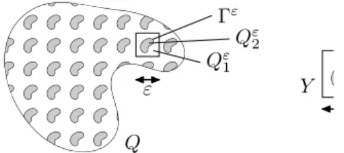
2.1. Geometric setting. Throughout this article, we will consider a bounded and open domain Q ⊂ R

³

. Furthermore, consider Y := [0, 1[

³

, with Y = Y

1

∪ Y

2

∪ Γ such that Γ := ∂Y

1

∩ ∂Y

2

∩ Y . We expand Y , Y

₁

, Y

₂

and Γ periodically to R

³

assuming that the periodizations of Y

₁

and Y

₂

are both simply connected and open in R

³

and Γ := ∂Y

1

∩ ∂Y

2

. We multiply the resulting structures by ε to obtain Y

^ε₁

= εY

₁

, Y

^ε₂

= εY

₂

and Γ

^ε

= εΓ. Finally, we define the following subsets of Q:

Q

^ε₁

:= Q ∩ Y

^ε₁

, the pore space, and Q

^ε₂

:= Q ∩ Y

^ε₂

, the solid matrix. Wherever it will not provoke any confusion, we equally denote Γ

^ε

:= ∂Q

^ε₁

∩ Q. The definitions are illustrated in figure 2.1. The outer normal vector of Y

1

on Γ will be called n

Γ

and the outer normal vector of Q

^ε₁

on Γ

^ε

is denoted as n

_Γ^ε

.

One should be very careful in not mixing up the periodic cell Y with the notion of a so called

“Representative Elementary Volume” (REV) that is used in applied sciences such as soil physics. The

REV is a volume that is big compared to micro structures but small compared to the macroscopic

scale. Therefore, a single cell εY is not suitable, neither Y . For example, Joekar-Niasar et. al.

1 ε

Γ Y₂ Y₁ Γ^ε

Q^ε₂ Q^ε₁

Q

Y

Figure 2.1. Sketch of geometrical setting and notation.

[28] found in their simulations, that an REV is at least of the size 40 × 40 × 40 periodic cells. An introduction to the REV-averaging method can be found for example in the book by Dormieux, Kondo and Ulm [11]; it should not be mixed up with the present method of formal asymptotic expansion.

However, given such Q, Y

^ε₁

and Y

^ε₂

, we identify εL

₀

as the parameter describing the typical size of a pore, where w.l.o.g. L

0

= 1 is the macroscopic length scale. With respect to application, ε is depending on the physical size of the pores and the complexity of the geometry, which is represented by Y , Y

1

and Y

2

. In any case, from the physical point of view, ε is a fixed parameter. In order to derive two-scale models, it is important to seek for a suitable non dimensionalization of the physical equations. This is topic of section 5.

2.2. Differential Operators on the Boundary. On Γ, let n

_Γ

be the normal vector field and for each arbitrary vector field a : Γ → R

³

, we define the normal part a

n

and the tangential part a

τ

via

a

_n

:= a · n

_Γ

, a

_τ

:= a − a

_n

n

_Γ

. We define the normal derivative of a scalar quantity a through

∂

_n

a := ∇a · n

_Γ

and the tangential gradient ∇

_τ

for such scalars through

∇

_τ

a := (∇a)

_τ

= ∇a − n

_Γ

∂

n

a . For any vector field f

_τ

tangential to Γ, we define the divergence

div

_τ

f

_τ

:= tr∇

_τ

f

_τ

. and we find:

div f = div

_τ

f + ∂

n

(f

_n

) . The mean curvature of Γ is defined as

κ

_Γ

:= trace (∇

_τ

n

_Γ

) and we find the following important result:

Lemma 1. (See for example [6]) For any f ∈ C

¹

(Γ) holds ˆ

Γ

∇

_τ

f = ˆ

Γ

f κ

_Γ

n

_Γ

+ ˆ

∂Γ

f ν

where ν

^∗

:= (n

_∂Q

)

_τ

and ν = |ν

^∗

|

⁻¹

ν

^∗

is the unit vector tangent to Γ and normal to ∂Γ. Further- more, for any tangentially differentiable field q holds

ˆ

Γ

div

_τ

q = ˆ

Γ

κ

Γ

q · n

Γ

+ ˆ

∂Γ

q · ν

Note that the Laplace-Beltrami operator on Γ is then defined by

∆

_{τ τ}

f = div

_τ

∇

_τ

f

and Lemma 1 yields for any continuously differentiable and tangential vector field f = f

_τ

on Γ (2.1)

ˆ

Γ

div

_τ

f = 0 .

3. Asymptotic Expansion and Darcy’s Law

Asymptotic expansion, as it will be applied below, is not a mathematically rigorous but only formal modeling tool. Given a microscopic geometry on Q by Y

^ε₁

, Y

^ε₂

and Γ

^ε

, it starts from a set of (partial) differential equations, the microscopic problem, which depends on the geometry and on ε. It is the aim of homogenization to investigate the behavior of solutions to the microscopic problem as ε → 0 and to identify approximating macroscopic or two-scale problems. In particular, the approximating problem often is not only defined on Q but on Q × Y although there are special cases where a reduction to a problem on Q is possible. This will be the case for the derivation of Darcy’s law below.

Note that there is big amount of literature on homogenization. Below, we will deal with ho- mogenization of Cahn-Hilliard-Navier-Stokes-Fourier systems, thus we get in touch with Stokes and Laplace operators. For former results on the homogenization of Navier-Stokes and Stokes flow, refer to works by Allaire [1, 2, 3], Ene and Saint Jean Paulin [12], Marušić-Paloka [32], Mikelić [33, 35], Sandrakov [44] and of course the pioneering work by Tartar in the appendix of [43]. For the ho- mogenization of diffusion and diffusion with nonlinear boundary conditions, the reader is referred to Amaziane, Goncharenko and Pankratov [5], Conca, Diaz and Timofte [9], Conca, Diaz, Liñan and Timofte [8], Heida [19], Hornung [27], Mikelić and Primicerio [34] and the references therein.

Considering any ε-dependent unknown u

^ε

, the basic idea of asymptotic expansion is an ansatz

(3.1) u

^ε

=

∞

X

i=0

ε

ⁱ

u

^ε_i

,

where the functions u

^ε_i

have to be specified. Since the domain Q = Q

^ε₁

∪ Q

^ε₂

∪ Γ

^ε

is characterized by, Q and Y = Y

1

∪ Y

2

∪ Γ and ε, it seems reasonable to assume that u

i

: [0, T ] × Q × R

³

→ R

^k

with u

_i

being Y -periodic in the third variable. In particular

u

_i

: [0, T ] × Q × Y → R

^k

(t, x, y) 7→ u

_i

(t, x, y) , with

u

^ε_i

(t, ·) := u

_i

t, ·, ·

ε

and (3.1) becomes

(3.2) u

^ε

(t, ·) =

∞

X

i=0

ε

ⁱ

u

_i

(t, ·, · ε ).

Additionally, the following relations for the gradient and the divergence operators hold:

(3.3) ∇ = ∇

_x

+ 1

ε ∇

_y

, div = div

_x

+ 1 ε div

_y

.

Inserting (3.3) together with (3.2) into the particular partial differential equation, separating powers of ε, we obtain effective equations for the approximate behavior of u

^ε

(t, ·) ≈ u

0

(t, ·). We will start by considering homogenization of the Stokes equations with the scaling introduced by Allaire [4]

(see also [27, chapter 3]).

3.1. Homogenization of the incompressible Stokes equation: Dynamic case. We start with the incompressible Stokes fluid. Incompressibility implies that the pressure p

^ε

is an unknown, density is constant and the velocity υ

^ε

has to fulfill the incompressibility condition (3.4b):

∂

_t

υ

^ε

− ε

²

div (µ∇υ

^ε

) + ∇p

^ε

= g

^ε

on Q

^ε₁

(3.4a)

div υ

^ε

= 0 on Q

^ε₁

(3.4b)

υ

^ε

= 0 on ∂Q

^ε₁

(3.4c)

υ

^ε

= 0 on Q

^ε₂

(3.4d)

With an additional initial condition on (0, T ] × Q of the form υ

^ε

(0, ·) = ˜ υ

₀

(·, ·

ε ) . We assume that g

^ε

(x) = g(x) and there is a family of functions

υ

_i

: [0, T ] × Q × Y → R

³

0 ≤ i < ∞ (t, x, y) 7→ υ

_i

(t, x, y)

p

_i

: [0, T ] × Q × Y → R

³

0 ≤ i < ∞ (t, x, y) 7→ p

_i

(t, x, y)

such that the solution υ

^ε

and p

^ε

can be described by υ

^ε

(t, ·) =

∞

X

i=0

ε

ⁱ

υ

i

(t, ·, · ε ) (3.5a)

p

^ε

(t, ·) =

∞

X

i=0

ε

ⁱ

p

_i

(t, ·, · ε ) (3.5b)

where the functions υ

_i

and p

_i

are periodic in Y . The first coordinate reflects the macroscopic behavior of the solution, while the second coordinate reflects microscopic variations due to presence of microscopic geometry. The basic Idea is to insert (3.5) together with (3.3) into (3.4a) and separate the terms by powers of ε such that equations (3.4) take the form

ε

⁻¹

(. . . ) + ε

⁰

(. . . ) + O(ε) = 0 . In particular, the result reads up to order 0:

(3.6a) ε

⁻¹

∇

_y

p

₀

+ ε

⁰

(∂

_t

υ

₀

− div

_y

(µ∇

_y

υ

₀

) + ∇

_x

p

₀

+ ∇

_y

p

₁

− g) + O(ε) = 0 (3.6b) ε

⁻¹

div

_y

υ

0

+ div

_x

υ

0

+ div

_y

υ

1

+ O(ε) = 0

(3.6c) X

i

ε

ⁱ

υ

i

(t, x, ·) = 0 on ∂Y

1

, X

i

ε

ⁱ

υ

i

(t, ·, y) = 0 on ∂Q

For each power of ε, a new set of equations is obtained, which has to hold independently on ε.

Order −1 of (3.6a) yields ∇

_y

p

₀

= 0. For order 0 of that same equation, the resulting system with order −1 in (3.6b) reads

∂

_t

υ

₀

− div

_y

(µ∇

_y

υ

₀

) + ∇

_x

p

₀

+ ∇

_y

p

₁

= g

div

_x

υ

₀

= 0

div

_y

υ

0

= 0 .

This is a complete two-scale model for υ

0

and represents as such a solution to the homogenization problem. Thus, we can consider either

υ

₀

(·, ·

ε ) or υ

_{ef f}

:=

ˆ

Y

υ

₀

(·, y) dy

as an approximation of υ

^ε

(·), where the quality of this approximation is measured in terms of

υ

^ε

(·) − υ

₀

(·, · ε )

L²(Q)

or kυ

^ε

(·) − υ

_{ef f}

(·)k

_L2(Q)

.

However, in laboratory experiments and in nature, we are interested the macroscopic behavior of υ

ef f

. To obtain a macroscopic description for the evolution of υ

ef f

, we consider u

i

solutions to

∂

_t

u

_i

− div

_y

(µ∇

_y

u

_i

) + ∇

_y

Π

_i

= e

_i

on ]0, T ] × Y

₁

div

_y

u

i

= 0 on ]0, T ] × Y

1

u

i

(0, ·) = 0 on Y

1

u

_i

(·, ·) = 0 on [0, T ] × ∂Y

₁

where e

i

is the i-th standard basis vector of R

³

. We furthermore introduce υ ˆ through ˆ

υ(t, x, y) :=

ˆ

_t

0

X

i

[∂

t

(g − ∇

_x

p

0

)

_i

(s, x)] u

i

(t − s, x, y)ds . Since

∂

_t

υ(t, x, y) = ˆ ˆ

_t

0

X

i

[∂

_t

(g − ∇

_x

p

₀

)

_i

(s, x)] ∂

_t

u

_i

(t − s, x, y)ds

+ X

i

[∂

t

(g − ∇

_x

p

0

)

_i

(t, x)] u

i

(0, x, y) , we find due to the initial conditions on u

_i

:

∂

_t

υ ˆ − div

_y

(µ∇

_y

υ) = ˆ g − ∇p

₀

− ∇

_y

ˆ

_t

0

X

i

[∂

_t

(g − ∇

_x

p

₀

)

_i

(s, x)] Π

_i

ds , and the velocity field can be split up into

υ

0

= ˜ υ + ˆ υ where

∂

t

υ ˜ − div

_y

(µ∇

_y

υ) + ˜ ∇

_y

q

₁

= 0 on (0, t) × Y

1

div

_y

υ ˜ = 0 on (0, t) × Y

1

˜

υ = 0 on (0, t) × Γ

˜

υ(0, ·) = a(·) on Y

₁

. Defining

A

_i,j

:= ∂

_t

ˆ

Y1

u

_i

· e

_j

one may check by partial integration, the initial conditions on u

i

and the assumption (g − ∇p)

t=0

= 0 that

υ

_{ef f}

= ˆ

Y1

˜ υ +

ˆ

_t

0

A(t − s) (g − ∇

_x

p

₀

) (s)ds ,

where υ ˜ → 0 pointwise as t → ∞. For a rigorous proof of this homogenization result refer to Allaire

[27, chapter 3].

3.2. The Stationary Case. For the stationary case in (3.4), i.e. ∂

t

υ

^ε

= 0, we end up with [27]

υ

_{ef f}

= ˆ

Y

υ

₀

= A (g − ∇

_x

p

₀

) where

A

_i,j

:=

ˆ

Y1

u

_i

· e

_j

and u

i

are solution to

−div

_y

(µ∇

_y

u

_i

) + ∇

_y

Π

_i

= e

_i

on Y

₁

div

_y

u

i

= 0 on Y

1

u

i

(x, ·) = 0 on ∂Y

1

. 4. Continuum Mechanics

We follow the outline of previous works by Heida, Málek and Rajagopal [23, 22] on phase field models as well as [20], where the author introduced a new method to derive thermodynamically consistent boundary conditions for phase field models.

4.1. The Porespace. Thus, on Q

^ε₁

, we assume the presence of a mixture consisting of two different (almost) immiscible species, which we call without loss of generality water and air, having partial densities %

w

and %

a

. Assuming mass conservation for both species and transported by partial velocities υ

_w

, υ

_a

we obtain mass balance equations of the form

(4.1) ∂

t

%

i

+ div (%

i

υ

i

) = 0 i ∈ {a, w} .

In particular, we exclude production of air and water and chemical reactions, for simplicity. The densities %

a

and %

w

add up to a total density % of the mixture and the momenta of air and water add up to the total momentum %υ, introducing by the same time the mean velocity υ of the mixture through:

% = %

a

+ %

w

, υ := 1

% (%

a

υ

a

+ %

w

υ

w

) . Therefore, we can formulate the mixture’s balance of mass as

∂

_t

% + div (%υ) = 0 .

Defining the material derivative for scalars a and vectors f through (4.2) a ˙ := ∂

_t

a + υ · ∇a, f ˙ := ∂

_t

f + (∇f ) υ we get with

c := %

w

% , j := (υ

w

− υ) %

w

and (4.1)

_w

:

% c ˙ + div j = 0 .

Following the approach by Heida, Málek and Rajagopal [23, 22], we are not interested in the balance of energy, momentum and angular momentum for each constituent but postulate that the mixture is sufficiently described by the balance of energy, momentum and angular momentum for the mixture as a whole. As pointed out in [23], this is useful if we are not interested in energy and momentum exchange between the several constituents.

Thus, introducing the Cauchy stress T , the internal energy per mass u, the total energy per mass E :=

¹₂

υ

²

+ u, the diffusive heat flux j

_E

, external energy supply s and external body force g, we require the validity of the following set of equations:

∂

t

(%υ) + div (%υ ⊗ υ) − div T = g T = T

^T

∂

_t

(%E) + div (%Eυ) − div ( T υ + j

_E

) = s .

As pointed out in [23], introducing

h := T υ + j

_E

leads to the system

(4.3) % ˙ + %div υ = 0 % υ ˙ − div T = g T = T

^T

% c ˙ + div j = 0 % E ˙ − div h = s .

While up to now, these equations do not account for any interaction between the two constituents water and air, note that such information will enter due to constitutive equations on T , j and h which will be derived below.

4.2. The Solid Matrix. On Q

^ε₂

, the solid Matrix, the velocity field is zero, the density is stationary and we do not consider any dynamics except for energy transport. Writing E

2

for the energy per volume in Q

^ε₂

and h

2

for the diffusive energy flux, the balance of energy reads

(4.4) ∂

_t

E

₂

− div h

₂

= 0 ,

as we assume no external (external of Q) supply of energy to the solid matrix.

4.3. The Microscopic Boundary. Following [20], we assume the presence of a surface energy field E

_Γ

on Γ

^ε

and assume that it evolves due to

(4.5) ∂

_t

E

_Γ

− div h

_Γ

=

⊕

E where h

Γ

is some surface energy flux and

⊕

E is supply of energy from the bulk to Γ

^ε

. Note that E

Γ

is not the trace of E or E

2

on Γ

^ε

. Indeed, E is measured in energy per mass, E

2

is measured in energy per volume and E

_Γ

in energy per area. However, due to h, h

₂

and

⊕

E, there is an exchange of energy between Q

^ε₁

, Q

^ε₂

and Γ

^ε

, as demonstrated in section 6.1.

As will be shown in section 7 we also have to account for an additional boundary condition for c which is of the form

(4.6) %∂

_t

c + %υ

_τ

· ∇

_τ

c =

^⊕

c .

5. Non-Dimensionalization

The equations of balance for %, c and E in system (4.3) can be brought to a form (5.1) ∂

t

φ + div (υφ) + div j

_φ

= 0 , φ ∈ {%, c, E}

while the balance of momentum takes the form

(5.2) ∂

_t

(%υ) + div (%υ ⊗ υ) − div T = g .

We want to study the behavior of these equations with respect to the characteristic scales of the physical setting: We assume that the characteristic scale of space is given by L

0

, the characteristic scale of time is given by t

₀

and the characteristic scales of %, c, E, υ, j

_φ

and T by %

^∗

, c

^∗

, E

^∗

, υ

^∗

, j

_φ^∗

and T

^∗

respectively. (Note that these scales may depend on ε as they may depend on the ratio between macroscopic and microscopic length scales. Furthermore, note that υ

^∗

, j

_φ^∗

and T

^∗

are scalars!) The non dimensionalized quantities are indicated by an upper index ε, thus by φ

^ε

, υ

^ε

, T

^ε

, j

^ε_φ

. We find

φ = φ

^∗

φ

^ε

, υ = υ

^∗

υ

^ε

, T = T

^∗

T

^ε

, j

_φ

= j

_φ^∗

j

^ε_φ

, and insert these relations in (5.1) and (5.2), having in mind

div = L

⁻¹₀

div

^∗

, ∇ = L

⁻¹₀

∇

^∗

, ∂

t

= t

⁻¹₀

∂

_t^∗

,

where div

^∗

, ∇

^∗

and ∂

_t^∗

are derivatives with respect to

_L^x

0

and

_t^t

0

. We find

∂

_t^∗

φ

^ε

+ t

0

υ

^∗

L

₀

div

^∗

(υ

^ε

φ

^ε

) + t

₀

j

_φ^∗

L

₀

φ

^∗

div

^∗

j

^ε_φ

= 0 , φ ∈ {%, c, E}

(5.3)

∂

_t^∗

(%

^ε

υ

^ε

) + t

₀

υ

^∗

L

₀

div

^∗

(%

^ε

υ

^ε

⊗ υ

^ε

) − t

₀

T

^∗

L

₀

%

^∗

υ

^∗

div

^∗

T = g . (5.4)

It is one of the most crucial steps in homogenization to identify the correct scales of the factors

(5.5) t

0

υ

^∗

L

₀

, t

₀

j

_φ^∗

L

₀

φ

^∗

, and t

0

T

^∗

L

₀

%

^∗

υ

^∗

.

In classical approaches to homogenization, these scales are identified after the constitutive equa- tions for j, h and T in (4.3) have been provided from theory.

However, there is one problematic issue connected with this approach: Even if constitutive equa- tions have been derived from thermodynamic principles, it is by no means clear that the non- dimensionalization and identification of ε yields thermodynamically consistent systems of equations for all ε. If the scaling of the equations would lead to a violation of the second law for small ε, the resulting homogenized equations would not be thermodynamically consistent and make the result doubtable.

Therefore, we will follow a different path: We will start by identifying the reasonable scales for (5.5). Then, we will directly derive non-dimensionalized constitutive equations for j

^ε

, h

^ε

and T

^ε

, using (5.3), (5.4) and the method of maximum rate of entropy production.

First note that the scaling in front of the convective term is the same for all quantities. We will assume that convection is small on the macro scale, i.e. that infiltration rates to the porous medium are low. Thus, it is assumed that

t

0

υ

^∗

L

0

= ε . Concerning

_L^t0j∗

0%^∗c^∗

in the balance equation for c

^ε

, note that we assume the transition zone to be small even compared to the diameters of the pores. Since j and j

^ε

basically determine the thickness of this transition zone, the scaling factor should be at least of order ε

¹

:

t

0

j

^∗

L

0

%

^∗

c

^∗

= ε .

Similarly, T

^ε

describes the interactions of the fluid inside the pores and we equally get t

0

T

^∗

L

0

%

^∗

υ

^∗

= ε .

The dissipative energy flux, is a far reaching effect and behaves differently. In particular, we assume in the following that

t

₀

h

^∗

L

0

%

^∗

E

^∗

= 1 .

Furthermore, for simplicity of notation, we drop the upper index ∗ in the differential operators div

^∗

,

∇

^∗

and ∂

_t^∗

and obtain the following non dimensionalized set of equations in Q

^ε₁

:

(5.6)

∂

t

(%

^ε

c

^ε

) + εdiv (%

^ε

c

^ε

υ

^ε

) + εdiv (j

^ε

) = 0

∂

t

%

^ε

+ εdiv (%

^ε

υ

^ε

) = 0

∂

_t

(%

^ε

υ

^ε

) + εdiv (%

^ε

(υ

^ε

⊗ υ

^ε

)) − εdiv T

^ε

= g

^ε

∂

_t

(%

^ε

E

^ε

) + εdiv (%

^ε

E

^ε

υ

^ε

) − div h

^ε

= g

^ε

· υ

^ε

, where it is assumed that j

^ε

has its major impact on the porescale as well as T

^ε

.

On Q

^ε₂

, we apply a similar procedure to the balance of energy (4.4) and obtain

∂E

₂^ε

− div h

^ε₂

= 0 .

Finally, on Γ

^ε

, we obtain for balance of E

Γ

and c the non dimensionalized equations

∂

t

E

_Γ^ε

− εdiv h

^ε_Γ

=

⊕

E

ε

%

^ε

∂

t

c

^ε

+ ε%

^ε

υ

^ε_τ

· ∇

_τ

c

^ε

=

^⊕

c

^ε

.

Finally, remark that due to above non dimensionalization, also the material derivative becomes a scaled operator and one obtains the following important relations:

˙

a = ∂

_t

a + ευ

^ε

· ∇a for scalars a , (5.7)

a ˙ = ∂

t

a + ε (∇a) υ

^ε

for vectors a , (5.8)

%

^ε

∇c ˙

^ε

= ∇%

^ε

%

^ε

(εdiv j

^ε₁

) − % (∇c

^ε

)

^T

(ε∇υ

^ε

) − div [(εdiv j

^ε₁

) I ] , (5.9)

where ∇c ˙

^ε

denotes the material derivative of ∇c

^ε

and will be used in section 7.

6. The Assumption of Maximum Rate of Entropy Production

Following Callen [7], Heida, Málek and Rajagopal [23] and Heida [20], we assume the existence of entropy fields η

^ε

, η

^ε₂

and η

_Γ^ε

having the following properties:

• η

^ε

= ˜ η(E

^ε

, υ

^ε

, %

^ε

, c

^ε

, ∇c

^ε

), η

₂^ε

= ˜ η

₂

(E

₂^ε

), η

_Γ^ε

= ˜ η

_Γ

(E

_Γ^ε

, c

^ε

, ∇

_τ

c

^ε

)

• Keeping all other parameters fixed, η, ˜ η ˜

2

and η ˜

Γ

are strictly monotone increasing in E

^ε

, E

₂^ε

and E

_Γ^ε

respectively. Thus, η(·, ˜ υ, %, c, ∇c), η ˜

₂

(·) and η ˜

_Γ

(·, c, ∇

_τ

c) are invertible for fixed parameters and we can assume

(6.1) E

^ε

= ˜ E(η

^ε

, υ

^ε

, %

^ε

, c

^ε

, ∇c

^ε

), E

^ε₂

= ˜ E

₂

(η

^ε₂

) and E

^ε_Γ

= ˜ E

_Γ

(η

_Γ^ε

, c

^ε

, ∇

_τ

c

^ε

)

• 0 ≤ ϑ

^ε

:=

^∂E_∂ηε^ε

, 0 ≤ ϑ

^ε₂

:=

^∂E_∂ηε^2ε

2

and 0 ≤ ϑ

^ε_Γ

:=

^∂E

ε Γ

∂η_Γ^ε

are strictly increasing with E

^ε

, E

₂^ε

or E

_Γ^ε

respectively, where we will assume for simplicity, that all three quantities coincide on Γ. In particular, for the traces of ϑ

^ε

and ϑ

^ε₂

on Γ

^ε

holds

(6.2) ϑ

^ε

|

_Γ^ε

= ϑ

^ε₂

|

_Γ^ε

= ϑ

^ε_Γ

on Γ

^ε

.

Thus, we denote all three quantities by ϑ

^ε

and call this quantity the temperature field of the system.

Having in mind (6.1), we calculate the material derivative of E and time derivatives of E

2

and E

Γ

through:

(6.3)

%

^ε

E ˙

^ε

= %

^ε

ϑ

^ε

η ˙

^ε

+ %

^ε

∂E

^ε

∂υ

^ε

· υ ˙

^ε

+ %

^ε

∂E

^ε

∂%

^ε

% ˙

^ε

+ ∂E

^ε

∂c

^ε

c ˙

^ε

+ ∂E

^ε

∂ (∇c

^ε

) · ∇c ˙

^ε

on Q

^ε₁

,

∂

_t

E

₂^ε

= ϑ

^ε

∂

_t

η

^ε₂

on Q

^ε₂

,

∂

t

E

_Γ^ε

= ϑ

^ε

∂

t

η

^ε_Γ

+ ∂E

^ε

∂c

^ε

∂

t

c

^ε

+ ∂E

^ε

∂ (∇

_τ

c

^ε

) · ∂

t

(∇

_τ

c

^ε

) on Γ

^ε

.

Inserting (4.3), (4.4), (4.5), (4.6) and (5.9) into (6.3) yields new balance equations for η, η

2

and η

Γ

of the form:

%

^ε

η ˙

^ε

= div q

^ε

ϑ

^ε

+ ξ

^ε

ϑ

^ε

on Q

^ε₁

,

∂

t

η

^ε₂

= div q

^ε₂

ϑ

^ε

+ ξ

^ε₂

ϑ

^ε

on Q

^ε₂

,

∂

t

η

_Γ^ε

= div

_τ

q

^ε_Γ

ϑ

^ε

+ ξ

^ε_Γ

ϑ

^ε

on Γ

^ε

,

where q

^ε_i

and ξ

_i^ε

will be provided below in section 7.

6.1. Global Balance of Energy and Entropy. For simplicity, we assume that Q is perfectly isolated, which means that any flux of mass, energy or entropy through ∂Q is excluded. Let n

_∂Q

be the outer normal vector of Q, we thus obtain the following conditions on ∂Q:

h

^ε

· n

_∂Q

= 0 h

^ε₂

· n

_∂Q

= 0 h

^ε_Γ

· n

_∂Q

= 0 q

^ε

· n

_∂Q

= 0 q

^ε₂

· n

_∂Q

= 0 q

^ε_Γ

· n

_∂Q

= 0 (6.4)

j

^ε₁

· n

_∂Q

= 0 υ = 0

Furthermore, it will be assumed that there is no net mass flux through the boundary Γ

^ε

, nor any chemical reaction at the boundary, i.e.

(6.5) υ

^ε

· n

_Γ^ε

= 0 and j

₁

· n

_Γ^ε

= 0 on Γ

^ε

.

The total energy E

^ε

and total entropy S

^ε

of the system are given as the integral of the respective fields on Q

^ε₁

, Q

^ε₂

and Γ

^ε

:

E

^ε

= ˆ

Q^ε₁

%

^ε

E

^ε

+ ˆ

Q^ε₂

E

₂^ε

+ ε ˆ

Γ^ε

E

_Γ^ε

, (6.6)

S

^ε

= ˆ

Q^ε₁

%

^ε

η

^ε

+ ˆ

Q^ε₂

η

₂^ε

+ ε ˆ

Γ^ε

η

^ε_Γ

, (6.7)

where the boundary integrals are assumed to enter of order ε since

ε→0

lim ε ˆ

Γ^ε

1 dx = ˆ

Q

ˆ

Γ

1 dx dy .

Note that this can be realized by choosing appropriate scales for E

_Γ^∗

and η

^∗_Γ

. Global changes of energy are assumed to be only due to work done by body forces. In particular, the global balance of energy reads:

0 = d dt E

^ε

−

ˆ

Q^ε₁

g

^ε

· υ

^ε

= ˆ

Q^ε₁

%

^ε

E ˙

^ε

+ ˆ

Q^ε₂

∂

t

E

₂^ε

+ ε ˆ

Γ^ε

∂

t

E

_Γ^ε

− ˆ

Q^ε₁

g

^ε

· υ

^ε

= ε ˆ

Γ^ε

1

ε (h

^ε

− h

^ε₂

) · n

_Γ^ε

+ εdiv

τ

h

^ε_Γ

+

⊕

E

ε

. (6.8)

Due to (6.4) and lemma 1 holds ˆ

Γ^ε

div

_τ

h

^ε_Γ

= ˆ

∂Q∩Γ^ε

h

^ε_Γ

· n

∂Q

= 0 ,

and due to the reasons pointed out in [20], equation (6.8) implies the local energy conservation

²

(6.9) 1

ε (h

^ε

− h

^ε₂

) · n

Γ^ε

+

⊕

E

ε

= 0 . The time derivative of global entropy with respect to time yields:

Ξ

^ε

:= d dt S

^ε

=

ˆ

Q^ε₁

ξ

^ε

ϑ

^ε

+

ˆ

Q^ε₂

ξ

^ε₂

ϑ

^ε

+ ε

ˆ

Γ^ε

1

ε ϑ

^ε

(q

^ε

− q

^ε₂

) · n

_Γ^ε

+ ξ

_Γ^ε

ϑ

^ε

= ˆ

Q^ε₁

ξ

^ε

ϑ

^ε

+

ˆ

Q^ε₂

ξ

^ε₂

ϑ

^ε

+ ε

ˆ

Γ^ε

ξ

^ε_Γ,tot

ϑ

^ε

, (6.10)

2We shortly repeat the original argumentation with slightly modified formulas: As pointed out in [20], “the reason why divτh^ε_Γ does not appear in (6.9) is twofold: First, due to lemma 1, it is possible to add ´

Γεdivτf_τ of any tangential vector field f_τ in (6.8) without violating the equality. In particular, we could equally derive a condition

1

ε(h^ε−h^ε2)·nΓ^ε+

⊕

E

ε

+rεdivτh^εΓ= 0for any r∈R. Second, it is reasonable to assume that absorption is a local process, i.e. that the energy supplyh^ε·nΓ^ε is first absorbed byΓ^εthrough

⊕

E

ε

and then dissipated throughh^ε_Γ, instead of being directly dissipated throughh^εΓ.”