Impacts of climate variability and climate change on renewable power generation

(1)

change on renewable power generation

Inaugural-Dissertation zur

Erlangung des Doktorgrades

der Mathematisch-Naturwissenschaftlichen Fakultät der Universität zu Köln

vorgelegt von Jan WOHLAND

aus Duisburg

(2)

Köln, 2019

(3)

Berichterstatter: JProf. Dr. Dirk WITTHAUT

Prof. Dr. Andreas SCHADSCHNEIDER

Prof. Dr. David BRAYSHAW

Vorsitzender der Prüfungskommission:

Prof. Dr. Thomas MICHELY

Tag der letzten mündlichen Prüfung: 12.06.2019

(4)

(5)

“The pessimist complains about the wind; the optimist expects it to change; the realist adjusts the sails.”

William Arthur Ward

“There is an urgent need to stop subsidizing the fossil fuel industry, dramatically reduce wasted energy, and significantly shift our power supplies from oil, coal and natural gas to wind, solar, geothermal, and other renewable energy sources.”

Bill McKibben

(6)

(7)

UNIVERSITY OF COLOGNE

Abstract

Faculty of Mathematics and Natural Sciences Department of Physics

Dr. rer. nat.

Impacts of climate variability and climate change on renewable power generation

by Jan WOHLAND

Anthropogenic climate change represents a major risk for human civilization and its mitigation requires reductions of greenhouse gas emissions. To stay consistent with the long-term temperature targets of international climate policy, global greenhouse gas emissions have to reach zero within a few decades. Such a dramatic transition towards sustainability in all sectors of human activity requires the decarbonization of power generation at an early stage. In absence of other viable technology choices and given the significant cost declines, renewable power generation forms the back- bone of the decarbonization. In contrast to thermal power plants, most renewables are not dispatchable but their generation dynamics are governed by the weather.

This dissertation adds to the quantification of impacts of climate variability on wind power generation on different time scales. In particular, it shows that interannual wind power generation variability already today has a strong influence on congestion management costs in Germany. Understanding this variability as a nor- mal system feature helps to prevent short-sighted reactions in legislation and power system design. Moreover, it is shown that relevant multi-decadal wind power generation variability exists. Owing to timescales of up to 50 years, these modes are not sufficiently sampled in any modern reanalysis (e.g., MERRA2 or ERA-Interim), which currently cover around 40 years. Consequently, power system assessments based on modern reanalyses may be flawed and should be complemented by multi- decadal assessments. In this context, I also show that 20th century reanalyses (ERA- 20C, CERA20C, 20CRv2c) disagree strongly and systematically with respect to long- term wind speed trends. The discrepancy can be traced back to marine wind speed observations which also feature strong upward wind trends that are likely due to an evolving measurement technique. As a consequence, 20th century reanalyses should be employed with care and cross-validation of results is recommended.

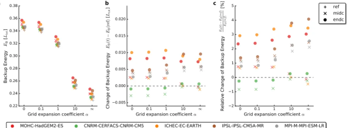
Due to their weather dependency, renewables are potentially vulnerable to climate change. Indeed, I show that the benefits of large-scale transmission infrastructure in Europe shrink under strong climate change (RCP8.5). The effect is robust across a five member EUROCORDEX ensemble and can be solidified in a larger CMIP5 ensemble. It is rooted in more homogeneous wind conditions over Europe that lead to less smoothing effects via large scale spatial integration.

Lastly, the debate around negative emission technologies to enlarge the carbon budget currently focuses on land-based approaches such as Bioenergy with Carbon Capture and Storage. Based on a schematic integration of Direct Air Capture (DAC), we show that its flexibility complements renewable generation variability and can help to integrate large shares of renewables.

(8)

(9)

Zusammenfassung

Menschengemachter Klimawandel stellt ein substantielles Risiko für die mensch- liche Zivilisation dar und seine Begrenzung erfordert eine Reduktion des Aussto- ßes von Treibhausgasen. Um mit den langfristigen Temperaturzielen des Pariser Klimaabkommens konsistent zu bleiben, müssen die globalen Treibhausgasemis- sionen in den nächsten Jahrzehnten auf Null reduziert werden. Ein solch tiefgrei- fender Übergang zu mehr Nachhaltigkeit in allen Sektoren menschlicher Aktivität erfordert die Dekarbonisierung des Strombereiches als einen der ersten Schritte. An- gesichts mangelnder vielversprechender alternativer Technologieoptionen und aufgrund des starken Rückgangs der Kosten stellen erneuerbare Energien das Rückgrat dieser Dekarbonisierung dar. Im Gegensatz zu den meisten konventionellen Kraft- werken, sind Erneuerbare allerdings nicht direkt steuerbar. Stattdessen wird die Dy- namik erneuerbarer Energieerzeugung vom Wetter diktiert.

Diese Dissertation trägt zur Quantifizierung von Einflüssen von Klimavariabili- tät auf Windenergieerzeugung bei und berücksichtigt dabei unterschiedliche Zeits- kalen. Insbesondere zeigt sie auf, dass interannuale Variabilität von Windenergieer- zeugung bereits heute einen starken Einfluss auf die Kosten von Engpassmanage- ment hat. Diese Variabilität als eine normale Eigenschaft des Systems zu verstehen hilft dabei kurzsichtige Reaktionen im Bereich der Gesetzgebung und dem Design des Stromssystems zu verhindern. Darüber hinaus wird gezeigt, dass es relevante multi-dekadische Windenergieerzeugungsvariabilität gibt. Da diese Moden Zeits- kalen von bis zu 50 Jahren aufweisen sind sie in allen modernen Reanalysen (z.B.

MERRA-2 oder ERA-interim) nicht ausreichend abgebildet, da moderne Reanalysen nur etwa die letzten 40 Jahre umfassen. Daraus folgt, dass Stromsystemanalysen, die auf modernen Reanalysen basieren, fehlerbehaftet sein können und mit multi- dekadischen Analysen ergänzt werden sollten. In diesem Zusammenhang zeige ich außerdem, dass Reanalysen des 20. Jahrhunderts (ERA20C, CERA20C, 20CRv2c) sich hinsichtlich langfristiger Windtrends deutlich und systematisch widersprechen.

Der Widerspruch kann auf marine Windbeobachtungen, die ihrerseits bereits deut- liche Aufwärtstrends beinhalten, zurückgeführt werden. Der Grund für die Trends ist wahrscheinlich eine sich entwickelnde Messtechnik, insbesondere eine systema- tische Verschiebung der Höhe des Messung. Es folgt, dass Reanalysen des 20. Jahr- hunderts vorsichtig verwendet werden sollten und dass eine Validierung der Ergeb- nisse durch Vergleich mehrerer Datenquellen zu empfehlen ist.

Aufgrund ihrer Wetterabhängigkeit sind Erneuerbare potentiell gefährdet durch den Klimawandel. In der Tat zeigen wir, dass die Vorteile eines großskaligen Strom- netzes unter starkem Klimawandel (RCP8.5) reduziert werden. Der Effekt ist robust innerhalb eines EUROCORDEX Ensembles mit fünf Mitgliedern und kann weiter untermauert werden in einem größeren CMIP5 Ensemble. Der Effekt hat seinen Ursprung in gleichmäßigeren Windbedingungen über Europa, die weniger ausglei- chende Effekte durch großskalige räumliche Integration ermöglichen.

Als letzter Themenbereich wird die Debatte um negative Emissionen aufgegrif- fen, die benötigt werden um das geringe verbleibende CO2Budget zu vergrößern.

Diese Debatte konzentriert sich zum Großteil auf Bioenergie mit CO₂ Abscheidung und Speicherung. Wir zeigen mittels eines schematischen Ansatzes zur Integration von CO2 Abscheidung aus der Luft (DAC), dass die Flexibilität von DAC und die Variabilität von Erneuerbaren sich ergänzen, sodass DAC helfen könnte große An- teile von Erneuerbaren in das Stromsystem zu integrieren.

(10)

(11)

Acknowledgements

This thesis would not have been possible without the continued support of many people. On the professional side, I want to thank JProf. Dr. Dirk Witthaut for countless valuable discussions, his general optimism and his willingness to inter- pret stupid regulations loosely. In the early phases of the thesis, Dr. Mark Reyers provided much support as did Prof. Dr. Noel Keenlyside and Dr. Nour-Eddine Om- rani in the later parts. I also want to thank Noel for hosting me as a visiting PhD student at the Geophysical Institute in Bergen. I thank the Hitec Graduate School at Forschungszentrum Jülich, namely Marianne Feldmann and Maurice Nuys, for funding this visit. I owe gratitude to Dr. Carl-Friedrich Schleussner for a refreshing cooperation and Prof. Dr. Martin Greiner for feedback and support. Many thanks also go to my fellow PhD students for shared coffee breaks and laughs!

Even though not directly involved in the science, this thesis would have failed without loving support from Alicja. Thank you for sharing the ups and downs and supporting me in any phase!

On a similar note, I wouldn’t have been able to write this dissertation without help from my parents Hans and Monika. In addition to their obvious contribution to my physical existence, they supported me during all steps that preceded this text and encouraged me to follow my own path. It goes without saying that the latter part also applies to my sister Anne who just never gives up.

Thank you all.

(12)

(13)

Acronyms

20CR NOAA’s 20th century reanalysis

BECCS Bio-energy with Carbon Capture and Storage

CERA20C ECMWF’s coupled atmosphere and ocean reanalysis of the 20th century

CMIP5 Climate Model Intercomparison Project Phase 5

CO2 Carbon Dioxide

COP Conference of the Parties CSP Concentrating Solar Power

DAC Direct Air Capture

DSO Distribution System Operator

ECMWF European Centre for Medium-Range Weather Forecasts ERA20C ECMWF’s atmospheric reanalysis of the 20th century ERA20CM ECMWF’s free model run of the 20th century

EUROCORDEX Coordinated Downscaling Experiment - European Do- main

GCM General Circulation Model or Global Climate Model

GHG Greenhouse Gas

IPCC Intergovernmental Panel on Climate Change

MTM Multi-Taper Method

NAO North Atlantic Oscillation

NOAA National Oceanic and Atmospheric Administration (USA)

PV Photovoltaics

RCM Regional Circulation Model or Regional Climate Model RCP Representative Concentration Pathway

ROC Receiver-Operator Characteristics TSO Transmission System Operator

UNFCCC United Nations Framework Convention on Climate Change

(16)

(17)

Chapter 1

Introduction

This dissertation touches two of the central challenges of the early 21th century:

climate change and renewable energy. It also discusses the sometimes overlooked aspect of climate variability which deserves equal attention. It aims to shed light on their interactions in both expected and surprising ways using methods from time series analysis and statistics. Prior to the discussion of the research results, a few fundamentals are reviewed in the next sections to familiarize the reader with the relevant concepts in a straightforward manner. I start with a brief discussion of climate change, which is both one of the main reasons for the increased deployment of renewables and also a potential thread to highly renewable power systems. After a short review of climate variability which governs the dynamics of renewable power generation, I introduce the main tools and datasets that are used in the research section of this dissertation. The following subsection on energy transitions covers main aspects of renewable power generation and focuses on emissions and the property of dispatchability. The Introduction ends with an overview of the publications pre- sented in this thesis. It is complemented by a Methods section that introduces an advanced spectral analysis tool that could only be briefly described in the corre- sponding publication.

1.1 Climate change

Human activity since the onset of industrialization has added substantial amounts of carbon dioxide (CO₂) and other greenhouse gases (GHGs) to the atmosphere as a byproduct of economic development. Current levels of atmospheric CO2 exceed 400 parts per million (ppm), representing a 40% increase from a pre-industrial level of around 280 ppm. The current level of CO₂ in the atmosphere is unprecedented at least in the last 800 000 years (IPCC, 2013). This perturbation of atmospheric composition leads to an increased amount of longwave outgoing radiation that does not make its way to outer space but is absorbed and then partly re-emitted back towards the earth surface. This is commonly referred to as the greenhouse effect. The increase of atmospheric concentrations of GHGs induces a thermal disequilibrium of the planet which currently absorbs more energy than it emits. As compared to pre- industrial levels, global mean temperature has consequently risen by approximately 1^◦Cwith a current rate of change of around 0.2^◦Cper decade (IPCC,2018).

1.1.1 Observed climate change

The responses to the thermal disequilibrium are not restricted to higher tempera- tures. Instead, they are many-fold and many of them pose a risk to human civilization and are therefore reasons for concern. The climate system consists of complex

(18)

(ice) and the biosphere. In many of these subsystems, impacts of anthropogenic climate change can already be detected today.

For example, global mean sea-level has risen by around 20cm over the 20th century mostly as a consequence of thermal expansion and shrinking glaciers (IPCC, 2013)¹. Other contributions come from mass losses of the Antarctic and Greenland ice sheet and land water storage. The rates of ice loss from Antarctica and Green- land have both increased from 1992-2001 to 2002-2011. Moreover, there has been an increasing number of extreme weather and climate events, such as more frequent warm days and nights, an increased frequency of heat waves in Europe, Asia and Australia and an increased area that is effected by heavy precipitation events. Even though individual extreme events can not be directly attributed to climate change for methodological reasons, their increased likelihood due to climate change can be documented in some cases (e.g., Wergen and Krug,2010; Coumou and Rahmstorf, 2012; Wergen, Hense, and Krug,2014). Parts of the emitted CO2are dissolved in the ocean, leading to ocean acidification and putting some marine habitats such as reefs at risk (Hoegh-Guldberg et al.,2007). Moreover, the climate systems features some self-amplifying feedbacks that can lead to tipping point behaviour. Once a system is perturbed sufficiently strongly (i.e., beyond its tipping point), it does not return to its initial state but transitions to another state following its internal dynamics. The transition to the new state may be accompanied by unusually high rates of change and it can feature hysteresis or irreversibility. Some of these tipping points may have already been crossed, as, for example, indicated by a weakening of the thermohaline circulation in the North Atlantic (Rahmstorf et al.,2015; Caesar et al.,2018) or a potentially triggered Marine Ice Sheet Instability in West Antarctica (Favier et al., 2014). Note that there is an ongoing debate about the stability of the thermohaline circulation in the North Atlantic. In a modeling study that was based on a large CMIP5 ensemble, Weaver et al. (2012) found a consistent reduction of the circulation strength but no evidence of a complete shutdown. A complete shutdown, as seen earlier in simpler models, might be prevented by stabilizing feedbacks between atmosphere and ocean processes that were not properly captured before (Buckley and Marshall, 2016). However, there is also concern that the current generation of climate models does not represent ocean freshwater transports correctly which could lead to an overestimation of stability. The question of whether or not the real circulation could feature tipping point behaviour thus remains an open one (Buckley and Marshall,2016).

1.1.2 Future climate change

While some impacts of climate change can already be detected today, the bulk of it will occur in the future owing to the inertia of the climate system. The number one determinant of future climate change is the future evolution of GHG emissions and the resulting concentrations in the atmosphere. There is a large body of literature that investigates climate impacts under different GHG scenarios and the latest (and the upcoming) report of the Intergovernmental Panel of Climate Change (IPCC) is an excellent source to access this information (IPCC, 2013). This section does not aim to deliver a holistic overview of climate impacts. Instead, a few sea-level related examples are given in the following that shall illustrate the potential scale of climate impacts in the long run.

Even if global mean temperature was kept at its current value, roughly 1% of global land area will be below sea-level in 2000 years (Marzeion and Levermann,

(19)

2014). While settlements may be easily relocated on this time scale, also 6% of world heritage sites will be effected. Moving them will prove more complicated. The numbers increase if higher levels of warming are assumed. In a 3^◦C warmer world, for example, 25-36 countries will loose more than 10% of their territory and some of them will see more than half of their land below sea level. Even in scenarios that are compatible with the long-term temperature goals of the Paris Agreement (see Sec. 1.1.3), sea-level rise in 2300 is expected to be at the order of one meter (Men- gel et al.,2018). Critical infrastructure that is deliberately installed next to the coasts, such as some power plants, is particularly prone to sea-level related risks (Bierkandt, Auffhammer, and Levermann,2015).

It has been mentioned earlier that parts of the West Antarctic Ice Sheet may have already entered a process called the Marine Ice Sheet Instability. This process requires a specific topography of the bedrock that the ice sheet rests upon. If looking upstream (i.e., towards the center of the ice sheet), the bedrock needs to slope downwards over some area. It has been shown that the destabilization of a part of the West Antarctic Ice Sheet is sufficient to trigger a process that culminates into its complete collapse (Feldmann and Levermann,2015). This would lock in irreversible sea-level rise of around 3m in the next millenia. The same process could unfold in parts of East Antarctica, which has long been thought to be significantly more stable. If an ice volume that is equivalent to around 0.008m sea-level rise is melted via external forcing, ice dynamics can induce the discharge of ice equivalent of 3-4m sea-level rise (Mengel and Levermann,2014). Sea-level rise in these orders of magnitude would require a fundamental reorganisation of infrastructures as many humans live next to the coasts.

Still more disastrous consequences are found if mankind was to use all fossil fuel resources that are currently considered available. The resulting forcing would trigger destabilization of the entire Antarctic ice sheet, ultimately releasing almost all of the ice that currently rests on the Antarctic continent (Winkelmann et al.,2015).

The multi-millenia sea-level response would exceed 50m and the rate of change in the first millennium would exceed 3m per century.

1.1.3 Safe climate change

In light of potentially disastrous impacts of unmitigated climate change, the United Nations Framework Convention of Climate Change (UNFCCC) was founded in 1992. It’s "ultimate objective (...) is to achieve (...) stabilization of greenhouse gas concentrations in the atmosphere at a level that would prevent dangerous anthropogenic interference with the climate system" (UNFCCC,1992). This sentence im- plicitly assumes that there is a threshold separating non-dangerous and dangerous interference with the climate system. What is this threshold? At which point does climate change end being safe?

It is important to understand that the threshold can not be determined by science alone because it depends on moral judgments. Whether or not a certain impact of climate change is acceptable has to be answered outside the world of science. However, science can contribute to the debate by differentiating the expected climate impacts at distinct levels of climate change. While the literature has focused on separating impacts in a 2^◦C to 5^◦C warmer world in the earlier phase of this century (e.g., Bank, 2012; IPCC,2013), the emphasis has shifted to compare impacts between 1.5^◦C and 2^◦C (e.g., Schleussner et al.,2016a; James et al.,2017; IPCC,2018). This shift is rooted in a large consensus that climate change beyond 2^◦C can not be considered safe.

(20)

The Paris Agreement and its carbon budgets

At the end of the 21st UNFCCC Conference of the Parties (COP), a multi-lateral climate change mitigation agreement was adopted (UNFCCC,2015). Named after the hosting city, the Paris Agreement contains ambitious goals for climate change mitigation and, at least in some sense, defines the threshold for dangerous interference.

In the second half of the 21st century, it aims for "a balance between anthropogenic emissions by sources and removals by sinks" of GHG. This implies a net GHG neu- tral world economy within a few decades and constitutes a tremendous challenge.

Regarding the long-term temperature goal, a compromise was found between countries that strongly argued in favour of limiting global warming to 1.5^◦C and those that wanted to stick to the more conservative 2^◦C target. The agreement contains both targets (“Holding the increase in the global average temperature to well below 2^◦C above pre-industrial levels and pursuing efforts to limit the temperature increase to 1.5^◦C above pre-industrial levels") and calls for a special report of the IPCC on global warming of 1.5^◦C that was published in late 2018. The choice of the long-term temperature goal was welcomed by members of the scientific community (Schellnhuber, Rahmstorf, and Winkelmann,2016).

An intuitive concept to illustrate the challenges in achieving the Paris Agree- ment’s goals is a carbon budget (Messner et al.,2010). It relies on the assumption that climate impacts are determined by cumulative GHG emissions, irrespective of the actual timing of emissions. This assumption has been shown to be a justified simplification in many cases (Zickfeld et al.,2009) although it obviously collapses if irreversible processes are triggered. A carbon budgetB(T)is an amount of carbon Bthat leads to exceedance of a temperature limit T if emitted into the atmosphere (T is the global mean temperature averaged over a long time span of two or three decades such that natural temperature variability can be neglected). After the budget is depleted, net carbon emissions of all sectors need to equal zero. According to the IPCC Special Report on 1.5^◦C (IPCC,2018), this budget is 550 GtCO2for a two- thirds chance to limit warming to 1.5^◦C. The budget estimate has a large uncertainty range of approximately±^{250 GtCO}2 dependent on non-CO₂ GHG mitigation and potentially−^{100 GtCO}2 to account for permafrost thawing and potential methane release plus another ±50% owing to a additional geophysical uncertainty due to non-CO₂response. More details of the uncertainties of climate budgets are provided in Millar et al. (2017). This budget compares to current rates of carbon emissions of B˙ ≈ ^{35 GtCO}2/y (Rogelj et al.,2015). If emissions remain constant, the entire budget of staying below 1.5^◦C with a 66% chance will thus be used in the 2030s. The budget is larger for the less ambitious 2^◦goal which translates into more time until it is finally used up.

The small size of these budgets calls for fast and fundamental changes of all sectors that emit carbon (Rockstroem et al.,2017) which includes, but is not limited to, the energy sector (Rogelj et al.,2015). Current levels of ambitions are not sufficient to reach the targets of the Paris Agreement (Schleussner et al., 2016b; Rogelj et al., 2016).

1.2 Climate variability

Climate variability is often also referred to as natural or internal variability. It de- scribes the dynamics of the climate system that would lead to climatic variations even in the absence of anthropogenic forcing. There are many different modes of

(21)

2017). Some modes are very slow and effect the entire planet such as the variations in orbital parameters that have led to glaciation events in the past with periods of approximately 23, 41 and 100 thousand years (Imbrie et al.,1992). They can be safely ignored for the purpose of this thesis. However, some dominant modes of climate variability feature multi-decadal variability that stems from interactions of the tro- posphere with the ocean and the stratosphere (Keenlyside et al.,2015; Omrani et al., 2016). We will see in publication #4 that multi-decadal variability is important for wind power generation (Sec.3.3.2). Some components of the climate system feature variability on short timescales that is restricted to small spatial areas such as wind gusts. Synoptic variability on timescales of a few days is one of the most important modes for the integration of renewables as passing weather systems can lead to fun- damentally different generation characteristics. The long-term evolution of synoptic variability is thus highly relevant for power system design.

Climate variability generally prohibits the attribution of individual events to climate change and complicates the attribution of trends that are observed or modeled over relatively short timespans. One reason is that low-frequency climate variability (i.e, multi-decadal, centennial and beyond) can produce signals that feature statistically highly significant trends over timespans that are substantially shorter than their period. For example, if the available timeseries only samples parts of the natural variability, trends may be found in a period with an upward or downward tendency. Such trends are not representative for the entire process but only capture the dynamics over a short period. They can not be safely generalized.

There is a direct link between climate variability and renewable power generation because renewables depend on the weather. Wind parks remain idle without wind and solar panels require sunshine. The dependence of wind power generation on wind speeds is even non-linear, highlighting the importance of understanding wind speed dynamics to quantify wind power generation.

1.3 Tools and Datasets for climate assessment

1.3.1 Climate Models

The assessment of future climate requires numerical models and scenario assump- tions regarding GHG concentrations. To this end, different Global Climate Models (GCMs) have been developed in climate modelling groups. They typically contain the most important climate subsystems and solve the underlying differential equations in discretized space and time. Their global coverage comes with the advan- tages that boundary effects are of minimum importance but also limits the obtain- able resolution. For example, the GCM results from the Climate Modeling Intercom- parison Phase 5 (CMIP5) that informed parts of the research reported in this study (see Sec.3.1.1), have a typical resolution of around 1^◦, which is at the order of 100km (Taylor, Stouffer, and Meehl,2011).

If higher resolution is needed, as it is the case for local assessments, Regional Climate Models (RCMs) can be used to downscale the GCM results (e.g., Giorgi and Gutowski, 2015). A RCM is a climate model with a limited spatial domain (e.g., Europe) but significantly higher spatial resolution. Per design, a RCM always needs boundary data such as heat and mass fluxes which are typically provided by a GCM.

The combination of a driving GCM and a nested RCM is often referred to as a modeling chain and comes with some methodological weaknesses because uncertainties can propagate through the different steps of the chain.

(22)

Meaningful regional climate change assessments thus have to rely on ensembles of RCM-GCM combinations which allow to investigate the robustness of changes across models. An ensemble of different RCM-GCM combinations at high resolution is provided by the EUROCORDEX initiative (Jacob et al.,2014) and is used in our analysis (Sec. 3.1.1). Agreement of multiple models is considered indicative of the robustness of a result. Ideally, many GCMs should be used to drive many RCMs such that the effects of both modeling steps can be studied. This particularly includes an ensemble assessment of the GCM data which serves as an input to the RCMs. However, as climate models rely on high performance computers that are costly, sometimes compromises have to be made. For example, in our analysis of the effectiveness of European transmission infrastructure under strong climate change, we had to rely on a 5 member GCM-RCM ensemble in which the same RCM was used in all cases because a larger set was simply not available.

Alternative approaches to derive higher resolution data also exist. Main approaches are empirical-statistical downscaling (e.g., Hewitson et al.,2014) and statistical-dynamical downscaling (e.g., Reyers, Pinto, and Moemken, 2015). Both rely on the assumption that a relevant share of local-scale variability can be explained as a funtion of large-scale variability. In empirical-statistical downscaling, the mapping from large scale to local scale is established statistically. In statistical-dynamical downscaling, the mapping is calculated by running a RCM for a small set of typical configurations. Both methods allow for a computationally cheap downscaling of large datasets (e.g., GCM ensembles). In some cases, they are well suited to comple- ment GCM-RCM modeling chains or to replace the usage of RCMs if computational costs are prohibitive. Both methods, however, may face serious methodological issues if the mapping is not stationary and/or if interannual to multi-decadal variability is not properly accounted for (Hewitson et al.,2014).

Scenarios of atmospheric composition

Human behaviour is not modeled in GCMs. This means that the addition of greenhouse gases to the atmosphere via combustion of fossil fuels is not captured by the climate models but has to be provided exogenously. This is done in the form of scenarios and the most recent set of those are called representative concentration pathways (RCPs) (Vuuren et al.,2011). To be precise, RCPs prescribe the evolution of greenhouse gases in the atmosphere rather than the fluxes of greenhouse gases into the atmosphere. This approach has been taken to enhance comparability in GCM ensembles. Owing to different parameterizations, for example, of the carbon cycle, the same amount of GHGs emitted into the atmosphere leads to different GHG concentrations and thus different radiative forcing in different GCMs.

In this thesis, the business as usual RCP8.5 scenario is investigated. It assumes no mitigation efforts and has been chosen to test the vulnerability of transmission infrastructure to climate change because it is a worst case scenario. The name stems from the amount of additional radiative forcing through increased levels of greenhouse gas concentrations which equals 8.5 W/m²in 2100 (Riahi et al.,2011). RCP8.5 causes a global mean temperature increase of around 3.6^◦C to 5.8^◦C in 2100 as compared to pre-industrial levels (IPCC,2013). In studies other than sensitivity studies, scenario uncertainty is one of the major sources of uncertainty of climate projections in particular in the long run. For example, climate change impacts under the RCP2.6 scenario would be significantly different from those under RCP8.5 and nobody can forecast with certainty which emission trajectory will become reality. RCP2.6 in-

(23)

sources of uncertainty are model uncertainty (e.g., the choice of parameterizations and numerical schemes) and internal variability (Hawkins and Sutton,2009). A reduction of model uncertainty can be obtained through large ensembles of different models as explained in Sec.1.3.1.

1.3.2 Reanalyses

Climate information is needed in many applications. In addition to future scenarios that are computed using climate models, data about the past is often needed. Such data can be obtained directly from observations. For example, the German Weather Service (DWD) operates a network of stations that measure climate variables. Simi- lar services exist in most countries and the resulting station time series are typically readily available, for example, via web portals (Hewitson et al., 2017). However, the interpretation of station data is complicated. Among other reasons, this is due to the irregular sampling of stations in space, small-scale effects in the immediate vicinity of the stations, interruptions of operation, measurement errors and instru- mental drifts. In many cases, reanalyses are a more suitable source of information than observations are.

Reanalysis datasets are a mixture of observations and modeling outputs. They provide gridded data that is internally consistent (i.e., respects fundamental laws of physics such as the conservation of mass) and that has minimum deviation from the observations. In contrast to observations, reanalyses typically have global coverage and are provided on a regular grid. They thus come in a format that allows for easy usage in many applications. They are particularly useful if observations are not available, sparse and/or available only over a short time period. Reanalyses are retrospective by design because they need observations as input. The reanalyses used in this thesis cover approximately the last 40 years (modern reanalyses) or the last 110 to 150 years (20th century reanalyses). The names of the reanalyses and their respective benefits and shortfalls are extensively discussed in Sec3.

There are three important and fundamental differences between reanalyses and climate models that are relevant in the context of this thesis. First, climate models are generally not synchronized while reanalyses are. This means that it can not be expected that two different GCMs are in phase with respect to any mode of climate variability. In other words, there is no reason to assume that, for example, wind speeds in any location at any particular date are the same in two different GCMs. The situation is different for reanalyses because the assimilated observations are synchronized (or even identical). Consequently, the wind speeds at any given date in reanalysis 1 can be meaningfully compared to those in reanalyses 2. Second, reanalyses are generally more realistic because they are coupled to the real world through the assimilation of observations. This is particularly important if relevant processes are not captured in the models due to, for example, insufficient resolution or missing components such as the stratosphere. Third, the maximum timespan that can be covered by reanalyses is limited by the available observations while GCMs can be run for infinite periods (given infinite computational resources).

1.4 Energy transitions

As noted earlier, delivering on the Paris Agreement and avoiding dangerous climate change requires a zero emission world economy in a few decades. However, the evolution of global CO emissions over the last decades points upwards rather than

(24)

downwards. For example, the global emissions from electricity and heat generation have risen from around 8 GtCO2 in 1990 to almost 14 GtCO2 in 2015 (IEA, 2017a).

After global emissions had plateaued between 2014 and 2016, they increased by 1.6%

(2%) in 2017 (2018) (Figueres et al.,2018). In other words, the peak of global emission still has not been reached.

In 2015, the largest fraction of CO₂ emissions originated from the generation of electricity and heat (42%) followed by the transport sector (24%) and industry (19%) (IEA,2017a). These numbers illustrate that the decarbonization of power generation is not sufficient. Instead, emissions have to fall to zero in all sectors or remaining carbon emissions have to be offset by negative emission technologies. The prospects of one particular negative emission technology are discussed in Sec.3.4.1.

Even though the transition to a fully renewable power system is not enough, it is a logical starting point. This is because renewable generation technologies (a) are available at scale (Brown et al.,2018a), (b) have minimum lifecycle GHG emissions (Pehl et al.,2017), and (c) electricity can be used to substitute fuels in transport and industry (Welder et al.,2018). Moreover, onshore wind and solar photovoltaics are least cost options for power generation already today (IEA and IRENA,2017). On- shore wind even outperforms all other available types of generation in some loca- tions in terms of levelized costs of electricity. Further cost reductions are anticipated (Creutzig et al., 2017). Technical renewable potentials are also significantly higher than current primary energy and electricity demand. Wind power alone could provide enough electricity to meet the global demand for electricity and the potential of solar power is even large enough to support multiples of the world’s current primary energy demand (IPCC,2014).

1.4.1 Renewable power generation

Renewable power generation means the utilization of self-replenishing resources to generate electricity. It includes these technologies: solar photovoltaics (PV), concentrating solar power (CSP), wind power, hydropower, bioenergy and a few others that only play niche roles (IEA,2017b). Renewables are in contrast to conventional power generation that is based on burning fuels (e.g., coal, gas, oil, waste) or nuclear fission. Nuclear fusion will not become available in time to relevantly contribute to the initial decarbonization of power systems. Even the most optimistic scenarios reported by pro-fusion groups argue that "fusion can start market penetration around 2050 with up to 30% of electricity production by 2100" (EFD,2012). Given that fundamental questions of reactor design are still not answered, these estimates are to be taken as highly speculative. However, even if fusion technology was available to be deployed at scale in 2050, it would have to be incorporated into a highly renewable system. This would require nuclear fusion to be operated flexibly, adding another massive design challenge. On top of this, the economic case for nuclear fusions remains unclear.

All types of power generation can be classified as either dispatchable or non- dispatchable. Wind and PV are non-dispatchable meaning that they can not be switched on when needed. Instead power generation from wind and PV is inter- mittent as it follows the weather. Conventional power generation is generally dispatchable although there are ramping constraints that need to be respected. CSP and hydropower are situated in between. While CSP generally is non-dispatchable, the addition of thermal storage can make it dispatchable on timescales of up to a few days (Pfenninger et al., 2014). Pumped hydropower is dispatchable as long

(25)

FIGURE1.1: Power generation in Germany in one example week in early 2019. Different colors denote different generator technologies as defined in the legend. The illustration is taken fromenergy-charts.

deon 26/03/2019 with kind permission from Bruno Burger (Fraun- hofer ISE).

as constraints on its filling level are respected whereas run-off-river hydropower is generally non-dispatchable.

The German power generation during one example week in early 2019 is illus- trated in Fig.1.1. It displays different types of power generators and their variability.

Solar photovoltaics only generates electricity during daytime. While it contributes relevantly on the first four days as can be seen from the first four peaks, the contribution on the remaining days is small. The pattern of wind generation is different and partly complementary. Wind plays a minor role until the evening of the third day when wind power generation strongly increases. Following a period of medium contribution, feed-in from wind power is dominant over the last day. Hy- dropower plays a minor role. Of the dispatchable generators, brown coal, uranium and biomass are operated in baseload mode (i.e., constantly) for almost the entire week. Hard coal and gas are used flexibly to respond to changes in wind and solar generation.

The non-dispatchability of wind and PV constitutes the main challenge of build- ing highly to fully renewable power systems because a stable and reliable power supply is considered a necessity in many parts of the world. While it requires new thinking and new infrastructures, there is evidence that this challenge can be solved.

The main strategies to integrate high shares of renewables are well understood. They all share the idea of optimizing the energy system in light of renewable generation variability and thus require accurate representations of climate variability. The main strategies are:

1. Averaging over large areas using transmission infrastructure (e.g., Rodriguez et al.,2014; Rodriguez, Becker, and Greiner,2015; Rodriguez,2014; Andresen et al.,2012; Becker et al.,2014; Schlachtberger et al.,2017; Santos-Alamillos et al.,2017; Grams et al.,2017)

(26)

2. Averaging over time using storage infrastructure (e.g., Beaudin et al., 2010;

Díaz-González et al., 2012; Toledo, Oliveira Filho, and Diniz, 2010; Kittner, Lill, and Kammen, 2017; Pleßmann et al., 2014; Luo et al., 2015; Reuß et al., 2017)

3. Increased flexibility on the demand side and combination of different sectors, such as heat and electricity (e.g., Brown et al., 2018b; Huber, Dimkova, and Hamacher,2014; Kondziella and Bruckner,2016)

Flexible conventional power generation from backup infrastructure will be needed during the transition. In fact, Schlachtberger et al. (2016) argue that even relatively inflexible generators can contribute beneficially in the early steps towards fully renewable systems.

1.5 Overview of the publications and their research ques- tions

All publications in Sec. 3contribute to the research field outlined above. They all use climate information to quantitatively assess energy related questions and make use of time series analysis and statistics. The focus is always on wind energy even though system wide effects are also studied in some cases.

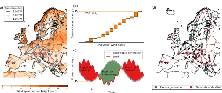
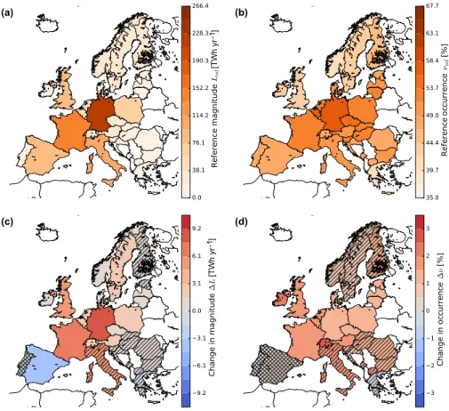
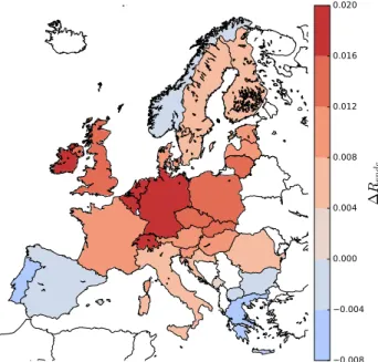
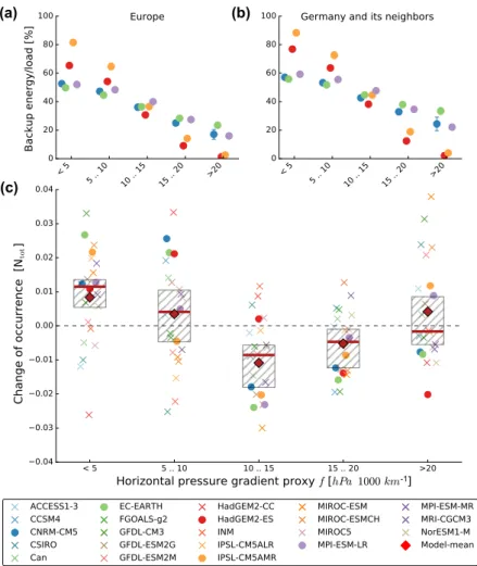
In publication #1 (Wohland et al., 2017), we investigate the impact of climate change on the smoothing effects of a continental transmission system in Europe. As explained in Sec. 1.4.1, large scale transmission infrastructure smooths the generation timeseries. This is because large areas are rarely affected by the same weather pattern simultaneously. Instead, below average wind generation in some countries often coincides with above average generation in others. In the paper, we ad- dress whether the benefits of large scale transmission are affected by strong climate change. We show that the effectiveness of transmission is robustly compromised under strong climate change at the end of the 21st century. The effect is rooted in more homogeneous wind conditions that imply higher synchrony of over generation and generation shortfalls across Europe. Albeit robust, the effect has a maximum ampli- tude of around 7% and is thus small enough not to prohibit highly renewable power system even under strong climate change.

Publication #2 (Wohland et al.,2018) addresses congestion management and as- sociated costs in the German electricity system. Due to transmission line constraints and a spatial mismatch of power generation and consumption, regulatory interven- tions to secure stable supply are sometimes needed. We focus on a measure called redispatch that has been used more extensively over the last years. Redispatch comes with annual costs at the order of a few hundred million Euros per year and is regu- larly discussed in the media. We contextualize an unexpected cost drop from 2015 to 2016 by comparison with expected inter-annual variability. The results highlight the importance of a proper inclusion of natural wind variability into energy policy and energy system design.

Publications #3 and #4 (Wohland et al.,2019a; Wohland et al.,2019b) both deal with multi-decadal wind assessments. They are based on 20th century reanalyses and aim to quantify whether any important modes of wind variability are missed in modern reanalysis. Owing to the methodological differences in approaches of the two providing centers of 20th century reanalyses, massive discrepancies in wind speed trends are reported in publication #3. Very strong upward trends are found

(27)

discrepancy to the assimilated wind speeds in the reanalyses that are provided by the European Centre for Medium-Range Weather Forecasts (ECMWF). Furthermore, based on a comparison with the literature and due to known issues with marine wind observations, we conclude that the upward trends in one family of datasets is likely spurious. After subtraction of the trends, agreement between the dataset is good as shown in publication #4. The corrected datasets feature significant multi- decadal modes of wind power generation averaged over the typical lifetime of a wind park. In particular, the ratio of winter to summer generation varies strongly (±15 %) which has direct implications for optimum technology choices.

In the last publication #5 (Wohland, Witthaut, and Schleussner,2018), we focus on a negative emission technology called direct air capture (DAC). Almost all scenarios that are compatible with the Paris Agreement require negative emissions to compensate exceedence of the carbon budget. In many models, negative emissions are reached via Bio-energy with Carbon Capture and Storage (BECCS), even though BECCS raises sustainability concerns owing to its large water and land footprint and resource competition with food production. We argue that DAC is a promis- ing candidate for negative emissions because it can be used flexibly and therefore complements renewable generation variability. We run a simple European power model to illustrate potentials of DAC for negative emissions and discuss co-benefits of storage and DAC.

During my PhD I also contributed to Weber et al. (2018) which is not discussed here. Moreover, another publication that I contributed to was accepted and published during the course of my PhD (Hewitson et al.,2017).

(28)

(29)

Chapter 2

Methods

The objective of this thesis is to distill robust information about impacts of climate variability and climate change on renewable power generation with a focus on wind energy. To this end, I use methods from time series analysis, statistics and uncertainty estimation based on cross-validation of suitable datasets. In general, all methods are introduced and discussed in the respective publication. They will not be repeated here for the sake of brevity. However, as the format of article #4 (Sec.3.3.2) did not allow to introduce the multi-taper method (MTM) in sufficient detail, additional information about MTM is given below. It starts with an introduction of spectral leakage which provides the motivation to use MTM.

2.1 Spectral leakage in finite length time series

In this section, we consider a univariate and discrete time seriesX(t)of finite length t= 1, ...,Nand time steps∆T. Often, the underlying dynamics of the timeseries are unknown (or too complex to be solved exactly). In such cases, a standard tool to investigate the properties of the time series is spectral analysis. Its easiest form is a discrete Fourier transform which is defined as

F{^X}(ω) =

∑∞ t=−∞

X(t)e⁻^i2πwt, (2.1)

whereωis referred to as frequency (e.g., Storch and Zwiers,1999).

As a trivial example, we know that the Fourier transform of a sinuisoid

X_example(t) =cos(2πω_examplet), (2.2) defined over an infinite period (t = −^{∞, ...,}∞), has a single peak at frequency ω_example:

F{^Xexample}=δ(ω= ω_example). (2.3) In real applications, however, time series are never of infinite length and rarely sufficiently long to justify the assumption of infinite length. For example in the climate context discussed in publication #4, we know that the length of the time series (110 years) only poorly samples the multi-decadal mode of a climatic process known as the North Atlantic Oscillation.

A finite length timeseries X^finite_example(t)can be considered as a combination of an

(30)

X^finite_example(t) =X_example(t)·^W(t). (2.4) The windowing function could, again following the easiest case, be a box:

W(t) =

(1, if t ∈[t_s,t_e]

0, otherwise (2.5)

Such a box could represent measurements over a finite period of time from t_s to t_e of an infinite process. The Fourier transform of the finite length time series, assuming the special caseω_example=0 for illustration, is

F{^X_example^finite (t)}=F{^Xexample(t)·^W(t)}=F{^cos(2π0t)

| {z }

=1

·^W(t)}= F{^W(t)}^. ^(2.6)

The Fourier transform of the finite length timeseries is thus directly effected by the window (cf. equations2.3 and2.6). While in this simple example, the Fourier transform of the finite length timeseries is even identical to the Fourier transform of the window, the exact influence of the windowing function on the spectra in more realistic cases cannot be seen as simply. However, from eq.2.6, it follows that

F{^X_example^finite (t)} 6= F{^Xexample(t)} ^(2.7) for most windowsW(t). This effect of the windowing function on the spectrum is called spectral leakage and the multi-taper method is one approach to minimize the effects of spectral leakage in finite time series.

2.2 Multi-taper spectral analysis

The entire section is based on Ghil (2002) unless stated otherwise. MTM consists of three steps.

First, a set of tapers (also referred to as windowing functions)

w_k(t), (2.8)

is calculated, and the total number of tapers is set by the user: k = 1, ...,K. The tapers are a discrete set of eigenfunctions that solve the variational problem to minimize spectral leakage outside a frequency band with half bandwidthp· ^fR, where f_R = _N_·¹_∆_Tis the Rayleigh frequency andpis another parameter. The definition of the tapers via the minimization problem implies that it is less heuristic than traditional techniques. The set of eigenfunctions is referred to as discrete prolate spheroidal sequences [Slepian, 1992].